A Homothetic Reference Technology in Data Envelopment Analysis by Ole B. Olesen

Discussion Papers on Business and Economics No. 14/2012

FURTHER INFORMATION Department of Business and Economics Faculty of Social Sciences University of Southern Denmark Campusvej 55 DK-5230 Odense M Denmark

ISBN 978-87-91657-67-2

Tel.: +45 6550 3271 Fax: +45 6550 3237 E-mail: [email protected] http://www.sdu.dk/ivoe

A Homothetic Reference Technology in Data Envelopment Analysis Ole B. Olesen(1) (1) Department of Business and Economics The University of Southern Denmark, Odense, Denmark, [email protected] August 13, 2012

Abstract Abstract: The assumption of a homothetic production function is often maintained in production economics. In this paper we explore the possibility of maintaining homotheticity within a nonparametric DEA framework. The main contribution of this paper is to use the approach suggested by Hanoch and Rothschild in 1972 to define a homothetic reference technology. We focus on the largest subset of data points that is consistent with such a homothetic production function. We use the HR-approach to define a piecewise linear homothetic convex reference technology. We propose this reference technology with the purpose of adding structure to the flexible non-parametric BCC DEA estimator. Motivation for why such additional structure sometimes is warranted is provided. An estimation procedure derived from the BCC-model and from a maintained assumption of homotheticity is proposed. The performance of the estimator is analyzed using simulation. Keywords: Data Envelopment Analysis (DEA), DEA Based Estimation of a Homothetic Production Function, Linear Programming, Convex Hull Estimation, Isoquant Estimation, Polyhedral Sets in Intersection and Sum Form JEL codes: C0, C4, og C6

1

Authors: O. B. Olesen

1

2

Introduction

Piecewise linear estimations in Data Envelopment Analysis (DEA) envelops observed data based on an axiomatic approach. Specifically, using the axiom minimal extrapolation an estimator of the technology is defined as the intersection of all technologies that satisfies the included axioms. An often used estimator in DEA is the BCC-estimator (Banker, Charnes and Cooper 1984), which maintains variable returns to scale (VRS) in the form of convexity and strong disposability. The minimal extrapolation principle implies that the BCC technology is estimated as the smallest convex set that contains all observed data points, and enlarged by strong disposability. However, it is well known, that piecewise linear estimators have slow convergence (Kneip, Park and Simar 1998). Hence, we will not expect to see shapes of the estimated isoquants conforming to the true shapes unless the sample size is sufficiently large relative to the dimension of the input output space. As illustrated in the next section, the shapes of the estimated piecewise linear isoquants can be very different from the true shapes if we only have access to a small sample of data points. In this paper we propose a homothetic convex reference technology within the framework of DEA. This contribution is based on the classical nonparametric test of homotheticity proposed in (Hanoch and Rothschild 1972). Below we will argue that one useful purpose of this "new" reference technology is to add structure to the flexible non-parametric BCC estimator. If this structure is in accordance with the true Data Generating Process (DGP) it is stipulated that the rate of convergence will increase. Starting from the BCC estimator1 we add structure to the shape of the estimated isoquants to "make up" for the problems of slow convergence and wrongly shaped isoquants estimated from small samples. Avoiding any a priory choice of a functional form is often stated as an important advantage of a non-parametric approach. However, fitting the observed data with the convex hull estimator could be seen as too conservative if we have some a priory information indicating a homothetic or near homothetic structure; it could e.g. be information on characteristics like i) the marginal rate of technical substitution, ii) the shapes of the expansion paths, iii) input separability, and with multiple inputs and outputs iv) input output separability (see (Hasenkamp 1976)). There are at least three reasons why a homothetic reference technology is an interesting extension to the classical DEA reference technologies: Firstly, using a non-parametric approach for an efficiency analysis it is interesting in its own right to analyze how much the estimated efficiency residuals are affected by an enlargement of the BCC-estimated possibility set resulting from an assumption of homotheticity. We often expect to have a technology with either linear of close to linear expansion paths which means that the assumption of a homothetic technology may be partly acceptable, at least as an approximation. We show below that the possibility set based on the convex hull estimation (the BCC model) is contained within the possibility set based on the proposed

Authors: O. B. Olesen

3

piecewise linear convex homothetic estimator which again is a subset of the convex cone estimator (the CCR model). Comparing the BCC and the CCR efficiencies provides the often used distinction between technical and scale efficiency, (Banker et al. 1984). Defining a homothetic VRS technology in between these two reference technologies allows us to further decompose the structure of inefficiency by estimating the radial distance to the homothetic frontier of points projected to the BCC frontier and by estimating the radial distance to the CCR frontier of points projected to either the BCC frontier or to the homothetic VRS frontier. Secondly, there are several empirical comparisons of nonparametric and parametric efficiency analyses, and the differences in reported rank correlations are remarkably large, see e.g. (Ferrier and Lovell 1990), (Resti 1997), (Cummins and Zi 1998), and (Bauer, Berger, Ferrier and Humphrey 1998). The parametric approaches used in such comparisons almost exclusively focus on economic efficiency2 based on a cost function estimation. At least in cases where rank correlations are low such discrepancies in the inefficiency structure could be a consequence of the chosen parametric functional form "picking up" some homothetic or near homothetic structure in data3 . The homothetic reference technology proposed in this paper can be used in the search for possible causes driving such low rank correlations. A homothetic reference technology allows for a comparison of a homothetic nonparametric cost efficiency estimation with the corresponding parametric cost function estimation. This clearly would be advantageous in cases where the parametric estimation cannot reject separability and homotheticity. But even in cases like (Resti 1997) where separability and homotheticity are rejected, a low rank correlation could be further explored by a comparison of parametric estimated cost efficiency and nonparametric homothetic based cost efficiency. More generally, the proposed homothetic reference technology provides a valuable tool in a comparison of a specific function form based Stochastic Frontier Analysis (SFA) and DEA. It allows for a specific analysis of the special case where homotheticity is imposed both on the parametric form (see (Berndt and Christensen 1973) or (Brown, Caves and Christensen 1979), page 259 for the case of a translog functional form) and on a DEA convex hull technology by enlarging the convex hull to fit a homothetic structure4 . This clearly extends the possibility of refining such comparisons. To further motivate the relevance of this new homothetic reference technology we illustrate in the following figures the impact of the slow convergence of a non-parametric estimated homothetic input structure. In section 8 we report simulation results from data generated from an input homothetic structure. The following Figure 1a -1d illustrate how the sample size affects the shape of the BCC-estimators of isoquants. With 50 or 100 observations we notice the distorted non-homothetic shapes. For larger sample size the typical homothetic shape of the isoquants becomes more prominent. Hence, in an analysis based on a relatively small sample size we would expect to see very different efficiency scores from a BCC envelopment of data

Authors: O. B. Olesen

4

compared to a parametric analysis based on a homothetic functional form. Input X2

Input X2

Sample Size: 100 Sample Size Eff DMUs: 35 Isoquant steps: 0.21

Sample Size: 50 Sample Size Eff DMUs: 28 Isoquant steps: 0.215

Input X1

Input X1 0

0

Input X2

Input X2

Sample Size: 500 Sample Size Eff DMUs: 79 Isoquant steps: 0.21

Sample Size: 1000 Sample Size Eff DMUs: 111 Isoquant steps: 0.2

Input X1 0

Input X1 0

Figure 1a,b,c,d. BCC Estimation of isoquants, Sample size 50,100,500,1000 Thirdly, a homothetic reference technology would allow a statistical testing procedure for homotheticity within the non-parametric production modeling approach. (Hanoch and Rothschild 1972) provide a test for homotheticity of a given data set. The test fails if the structure in data is inconsistent with a homothetic DGP. However, failing this test provides no inference, which implies that it is not possible to tell whether or not the deviation from a homothetic DGP is significant or not. (Primont and Primont 1996) and (Primont and Primont 1994) provide an extended testing procedure in relation to both input and output homotheticity, which does not assume that all observations are technical efficient. This test suffers from the same lack of inference. With an explicit homothetic reference technology we can either use the semi-parametric approach proposed in (Banker and Natarajan 2004) or a bootstrapping approach proposed by (Simar and Wilson 2002) to determine if the residuals from a BCC-envelopment are significantly different from the corresponding residuals from a homothetic extension of the BCC convex hull estimator. In addition the homothetic reference technology allows for an extension of the often used decomposition of overall efficiency into technical and scale

Authors: O. B. Olesen

5

efficiency. For a BCC inefficient DMU the overall inefficiency can be decomposed into a radial contraction to the BCC frontier, a further contraction to the homothetic frontier and finally a further contraction to the CCR-frontier. The approach proposed in this paper has one apparent shortcomings. To simplify the presentation we have assumed only one output. Generalizing the proposed input homothetic reference technology with one output to an output homothetic reference technology with one input is straight forward and is outlined in Appendix 2. But extending the proposed approach to a multiple output (input) in an input (output) homothetic reference technology is more complicated and is left for future research. The rest of the paper is organized as follows. In section 2 we define the production technology from an input orientation using an input distance function. The assumption of homotheticity is presented and several implications are discussed. Hanoch and Rothschild’s test for homotheticity is presented in Section 3, and extended to allow for inefficient observations. In Section 4 we define the homothetic reference technology and show that it is a proper subset of the BCC reference technology. Unfortunately, many alternative solutions for a homothetic reference technologies are available and several procedures to choose "a tight" solution are discussed. A small sample simulation is presented in Section 5 based on a homothetic DGP. The last section concludes with directions for future research

2

Definition of input-homotheticity

To simplify the presentation of a homothetic reference technology we focus almost entirely on an inputhomothetic production function, i.e. we focus on the situation with one output. In appendix 2 we will, however, briefly indicate how the reference technology proposed easily can be extended to the situation with one input (e.g. cost) and multiple output. Homothetic production functions first proposed by (Shephard 1953) have played an important role in production economics and several important features of such production functions are well known. A homothetic production function is equivalent to any expansion path being a ray from the origin. A homothetic production function is a monotonic transformation of a linear homogenous production function which in geometric terms means that any input isoquant from a homothetic production function simply is a radial rescaling of the unit isoquant. Let us consider a production environment where a vector of m inputs X = (x1 , . . . , xm ) is used in the production of one output Y . We represent the production technology with the input set L(Y ) = {X ∈ Rm + :X can produce Y } which has isoquant IsoqL(Y ) = {X : X ∈ L(Y ), λX ∈ / L(Y ), λ ∈ [0, 1)}.

(1)

Authors: O. B. Olesen

6

Since we assume that only one output is produced, we can define a production function as f (X) = max {Y : X ∈ L(Y )}. The input distance function is then defined as DI (Y, X) = max {γ : X/γ ∈ L(Y )} ,

(2)

which provides an alternative characterization of the technology since DI (Y, X) ≥ 1 ⇔ X ∈ L(Y ). Finally, the index of technical efficiency proposed by Debreu (1951) and Farrell (1957) that serves as basis for DEA is given as FI (Y, X) = min {γ : γX ∈ L(Y )},where FI (y, x) = DI (y, x)−1 . Definition 1 A production function f (X) is homothetic

Y = f (X) = F (g(X))

where F () : R+ → R+ is monotonic and g(λX) = λg(X) i.e. g() is positive homogeneous of degree one and continuously differentiable (see (Shephard 1970)). g() is denoted the kernel function. The following proposition (Olesen and Ruggiero 2012) shows that a homothetic production function can be represented as a production process whereby the input vector X can be aggregated into a one dimensional input index g(X), i.e. output is determined from the level of aggregate input (see (Färe and Lovell 1988) for a more general result). Proposition 1 Assume a homothetic technology with one output. The distance function evaluated at (1, X) is equal to aggregate input defined from the core function in the homothetic production function multiplied by a constant, i.e. DI (1, X) = k × g(X), k ∈ R+ In other words, under the assumption of homotheticity the dimensionality of DEA models can be reduced. In addition, homotheticity allows us to span the production technology from the input set associated with the unit isoquant L(1) (see (Shephard 1970), page 34).

L(Y ) = H(Y )L(1),

where H(Y ) =

F −1 (Y ) F −1 (1)

(3)

is a scaling function. Hence, input sets can be theoretically generated from a base

input set by the scaling function that depends only on the level of output and not the input mix. Similarly, we have from Proposition 1 that IsoqL(Y ) = H(Y )IsoqL(1) , i.e. we can in general generate any isoquant from the unit isoquant. More generally, we could choose any output level and its associated input isoquant

Authors: O. B. Olesen

7

to serve as the base.

3

Testing for Homotheticity

Let us consider a sample of n data points (Xj , Yj ) ∈ Rm+1 , j ∈ N ≡ {1, . . . , n}. Following (Hanoch and + Rothschild 1972) the main question is whether or not these data, or a subset of these data could have been generated from a homothetic production function, i.e. a homothetic Data Generating Process (DGP) with no inefficiency. If this is the case for a given subset then an estimator of the corresponding homothetic production function is warranted. The main contribution of this paper is to use the approach suggested by Hanoch and Rothschild to define a homothetic reference technology. However, we need explicitly to "allow" for inefficiency in data5 implying that we will not insist that all observations are consistent with a homothetic technology. We focus on the largest subset of data points that is consistent with such a production function. Secondly, focusing on homothetic production functions we will use the testing procedure to define a piecewise linear homothetic convex reference technology. If data is generated from a homothetic production technology a homothetic reference technology allows us to obtain more accurate efficiency scores which converge faster to the true efficiency. Following (Hanoch and Rothschild 1972) we focus on a production function f (x) : Rm + → R+ that satisfies the following axioms: Axiom 1 Consistency with observations: f (Xj ) = Yj , j ∈ N Axiom 2 (Weakly monotonicity) x ≥ x0 ⇒ f (x) ≥ f (x0 ) Axiom 3 (Quasi-concave and continuos from above) The input requirement sets for y : L(y) = {x : f (x) ≥ y} are convex and closed for any real y Axiom 4 The production function f (x) satisfies Axiom 1 and there exists input prices v j ≥ 0, vj 6= 0, j ∈ N such that f (Xj ) ≤ f (x) ⇒ vj Xj ≤ vj x Axiom 5 (Homotheticity) For the production function f (x) there is a positive increasing function λ (y) such that h (x) = λ [f (x)] is linear-homogeneous and concave. In this paper we focus on a convex homothetic reference technology (in the DEA tradition); hence, we maintain the follow axiom as well: Axiom 6 (Convexity) The production possibility set {(x, y) : f (x) ≥ y} is a convex set.

Authors: O. B. Olesen

8

The theorem used in (Hanoch and Rothschild 1972) to formulate the test for a homothetic DGP is: Theorem 1 Axioms 1,2,3,4, and 5 are equivalent to the existence of vj ≥ 0, v j 6= 0 and λj > 0, j ∈ N satisfying the following v j ≥ 0,

j∈N

v j Xj = λj ,

j∈N

v i Xj ≥ λj ,

i 6= j, i, j ∈ N

λj ≥ λi ,

if Yj ≥ Yi , i, j ∈ N

λ1 = v 1 Y1 Proof. See (Hanoch and Rothschild 1972) page 272. The following program (denoted the HR-test) provides a test for the existence of a homothetic DGP: min

β

s.t.

λj − λi

≥

0

i, j where Yj ≥ Yi , i, j ∈ N

(4.1)

vi Xj − λj + β

≥

0

i 6= j, i, j ∈ N

(4.2)

vj Xj − λj

=

0

j∈N

(4.3)

v1 X1

=

Y1

(4)

(4.4)

vi ∈ Rm + , i ∈ N, β ≥ 0 where a homothetic production function exists if and only if β ∗ = 0, with β ∗ being the optimal solution to (4). Otherwise β ∗ > 0 is a measure of the maximal violation of homotheticity. The constraint (4.4) is ³ ´ an arbitrary (but convenient) normalization6 . Axiom 5 implies that [λ (f (x))]−1 h (x) = h λ(fx(x)) = 1;

hence, input vectors rescaled by [λ (f (x))]−1 all belong to the unit isoquant. If Axiom 5 holds and β ∗ = 0

in (4) then the positive increasing function λ (•) evaluated at Yj can be chosen as the estimated λ∗j > 0 from ³ ´ X (4), implying from (4.3) that v j λjj = 1, j ∈ N . In other words from a specific set of optimal λ∗j > 0 the ³ ´ X corresponding rescaled input vectors λjj , j ∈ N, all belong to the unit isoquant. This rescaling approach will be used below to span a piecewise linear convex homothetic reference technologies as the convex hull of

all input output vectors and all rescaled input output vectors. Notice that viT Xj ≥ λj , i 6= j in (4.2) (with £ ¤ β ∗ = 0) implies that viT (λj )−1 Xj ≥ 1, i 6= j, reflecting the assumption of convex unit isoquants.

Authors: O. B. Olesen

4

9

Using the HR-test to get a homothetic reference technology.

The contribution of this paper is to use the structure of the HR-test to define a piecewise linear convex homothetic reference technology. To allow for this purpose, we must allow for inefficiency in data. For this reason the estimation of the maximum deviation β from homotheticity in (4) is not convenient. We replace the single maximal violation β with a DMU specific correction β j , j ∈ N which in optimum will measure the unit specific contraction of the input vectors necessary to bring the data set into a shape, which could have been generated from a homothetic technology. Secondly, the objective function is modified accordingly to be a minimization of the sum of the DMU specific deviations β j . Thirdly, we need additional structure to make sure that the technology is convex. The convex homothetic reference technology will be defined such that it will contain the convex hull from the BCC model as a (proper) subset. Hence, a first step for any data set is to remove all observations that are BCC-inefficient. Such observations clearly belong to the interior of any convex homothetic estimator of the technology. The second step is to identify a subset of BCC efficient DMUs (possibly empty) that is causing the HR-test to fail. In this second step we solve the following modified version of the HR-test7

min s.t.

P

vjT Xj − λj

=

0

j∈E

(5.1)

(λj − β j ) − (λi − β i )

≥

0

i, j where Yj ≥ Yi , i, j ∈ E

(5.2)

viT Xj − λj

≥

0

i 6= j, i, j ∈ E

(5.3)

≥

0

∀i, j, k where Yi ≤ Yj ≤ Yk , i, j, k ∈ E

(5.4)

=

Y1

j∈E β j

Yj −Yi (λj −β j )−(λi −β i )

−

Yk −Yj (λk −β k )−(λj −β j )

v1T X1

(5)

(5.5)

vj ∈ Rm + , β j ≥ 0, λj ≥ 0, j ∈ E where E ⊂N is the set of all weakly BCC efficient DMUs. All BCC efficient DMUs are consistent with a homothetic technology if and only if β ∗j = 0, j ∈ E. Notice that an additional set of constraints has been included as (5.4) reflecting that we insist that the technology is convex. In general, many different subsets of BCC efficient DMUs could possibly be identified in an attempt to find a subset of DMUs suitable to span a piecewise linear convex homothetic reference technology. In (5) we follow the econometric tradition and choose an optimal solution that minimize the sum of "residuals" over all weakly BCC efficient DMUs. Let us focus on the homothetic reference technology that can be spanned from weakly BCC efficient DMUj with j ∈ E0 ⊂ E, where DMUj satisfies the test (5), i.e. β ∗j = 0, j ∈ E0 . To ease the presentation we will assume the following (nonrestrictive) regularity condition:

Authors: O. B. Olesen

10

Condition 1 Let n1 = #(E0 ) be the number of weakly BCC-efficient DMUs with β ∗j = 0 in (5). The observed input output combinations (Xj , Yj ) , j ∈ E0 have n1 strictly different output levels, i.e. Yi 6= Yj , ∀i, j ∈ E0 , i 6= j. Obtaining an optimal solution to (5) allows us to project each of these n1 observed input vectors to each of the n1 − 1 other isoquants8 , using the optimal λ∗j , j ∈ E0 . A convex piecewise linear technology Thomothetic can now be obtained using the convex hull estimation on the following set of n1 × n1 either observed or rescaled observations ¡ ¢ Thomothetic λ∗1 , . . . , λ∗n1 = Conv

∙½µ

¶ ¾ ¸ λ∗j 0 m Xi , Yj , ∀i, j ∈ E + R+ × R− λ∗i

(6)

where Conv() is the convex hull operator. Notice, however that in general many different alternative optimal solutions are available from (5). Below we outline an approach where we choose among alternative solutions the one that minimizes the sum of the inefficiency residuals from the union of the set of BCC inefficient DMUs and the set of BCC efficient DMUs with β ∗j > 0 in (5), i.e. from N \ E0 . We have the following proposition: £ ¡ ¢ ¤ Proposition 2 Thom othetic λ∗1 , . . . , λ∗n1 ⊃ TBCC ≡ Conv {(Xj , Yj ) , ∀j ∈ N } + Rm + × R−

¡ ¢ Proof. We will show that (Xj , Yj ) ∈ Thomothetic λ∗1 , . . . , λ∗n1 , j ∈ N. If that is the case then clearly ¡ ¢ Thomothetic λ∗1 , . . . , λ∗n1 ⊃ TBCC .

Let us partition the DMUs into three sets: i) E0 , ii)E \ E0 , and iii)N \ E. ¡ ¢ Clearly any (Xj , Yj ) ∈ Thomothetic λ∗1 , . . . , λ∗n1 , j ∈ E0 .

Consider (Xjo , Yjo ) , jo ∈ E \ E0 . We know that the optimal values from (5) will give us that β ∗j = 0, j ∈ E0 ,

and β ∗jo > 0. We may interpret the optimal β ∗j > 0, j ∈ E \ E0 as the necessary adjustment of the input vectors of DMUj , j ∈ E \ E0 to bring the data set (Xj , Yj ) , j ∈ E into a form consistent with a homothetic DGP. W.l.o.g. let E0 = {1, . . . , n1 } and assume the regularity condition (Condition 1). This implies that ∃j1 , j2 such that Y1 < Y2 < . . . Yj1 < Yj0 < Yj2 < . . . < Yj#(E0 ) . A β ∗jo such that P λ∗j1 ≤ λ∗jo −β ∗jo ≤ λ∗j2 ⇔ λ∗jo −λ∗j1 ≥ β ∗jo ≥ λ∗jo −λ∗j2 is feasible in (5.2) and (5.4) and since we minimize j∈E β j ∙ ¸ ¡ ¢T β∗ in the objective function we get β ∗jo = λ∗jo − λ∗j2 ⇔ λ∗jo − β ∗jo = λ∗j2 ⇔ vj∗o Xjo − ∗ joT em = λ∗j2 , v ( jo ) em T where em = [1, . . . , 1] . ∙ ¸ n³ ´ o β∗ jo b bjo , Yjo , (Xj , Yj ) , j ∈ E0 Hence, if we replace Xjo with Xjo ≡ Xjo − ∗ T em the set of observations X (vjo ) em will pass the test of being consistent with a homothetic DGP. Let the new homothetic reference technol³ ´ ³ ´ b∗ where bjo , Yjo using (6) be denoted Thomothetic λ∗1 , . . . , λ∗n , λ ogy spanned by (Xj , Yj ) , j ∈ E0 and X jo 1 ∙ ¸ ∗ ¡ ∗ ¢T ¡ ∗ ¢T ¡ ¢ ∗ β T ∗ ∗ j ∗ b = v bj = v Xjo − ∗ oT em = λjo − β jo by construction. Since vjo Xjo − β ∗jo = λ∗j2 X λ jo o jo jo (vjo ) em

Authors: O. B. Olesen

11

b∗ = λ∗ which means that we have λ jo j2

³ ´ ¡ ¢ b∗ = Thomothetic λ∗ , . . . , λ∗ Thomothetic λ∗1 , . . . , λ∗n1 , λ jo 1 n1

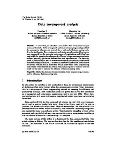
¡ ¢ which implies that (Xjo , Yjo ) ∈ Thomothetic λ∗1 , . . . , λ∗n1 . ¡ ¢ ¡ ¢ Finally, (Xj , Yj ) ∈ Thom othetic λ∗1 , . . . , λ∗n1 , j ∈ E, and since Thom othetic λ∗1 , . . . , λ∗n1 is a convex set by ¡ ¢ construction then clearly any convex combination of (Xj , Yj ) , j ∈ E belongs to Thomothetic λ∗1 , . . . , λ∗n1 , ¡ ¢ which implies that (Xj , Yj ) ∈ Thomothetic λ∗1 , . . . , λ∗n1 , j ∈ N \ E. ¡ ¢ Figure 2 illustrates TBCC and Thomothetic λ∗1 , . . . , λ∗n1 with two inputs and one output and 22 BCC efficient DMUs.

p

Co ve

u o

o ot et c ec o ogy

3 3

15

15

2

2 13

output

12

12

output

7

7 9 5

8

1

1

9 8

3

3

3 0 2

3 0

3

3 2 2

2

2 1 input1 1

1

0

input1

1

input2

input2

1 1

0 0

0

Figure 2. The BCC-technology and one solution of the corresponding homothetic technology, both spanned by 22 BCC efficient DMUs Next, let us characterize all alternative solutions to the homothetic reference technology in (6) generated from alternative solutions to (5). Consider the special situation where all BCC efficient DMUs are consistent with a homothetic DGP. In other words, E = E0 and any alternative basic solution in (5) can be generated 1 from one of the vertices in the following bounded polyhedral set9 of (v1 , . . . , vn1 ) ∈ Rm×n : +

Authors: O. B. Olesen

A≡

12

© 1 (v1 , . . . , vn1 ) ∈ Rm×n : +

viT Xj − vjT Xj ≥ 0, i 6= j, i, j ∈ E0 , Yj −Yi vjT Xj −viT Xi

−

Yk −Yj T X −v T X vk j k j

≥ 0, ∀i, j, k ∈ E0 where Yi ≤ Yj ≤ Yk ,

(7)

vjT Xj − viT Xi ≥ 0, j where Yj ≥ Yi , i, j ∈ E0 ª v1T X1 = 1

Notice that the polyhedral set A is a bounded convex polyhedral set in intersection form, i.e. A is expressed as the intersection of a finite number of inequalities and one equality. It is well known that any polyhedral set can either be expressed in intersection form or in sum form. A polyhedral set in sum form is a set expressed as convex combinations of vertices plus non-negative linear combinations of extreme rays, see the Appendix 1 for the Minkowski-Weyl’s Theorem. In the following alternative (non necessarily basic) solutions will be generated using convex combinations of the vertices of A. Hence we need to transform A to its corresponding sum form10 . Assume that the vertices of A are V k , k ∈ V. A can alternatively be expressed as: A=

(

v = (v1 , . . . , vn1 ) ∈

1 Rm×n +

:v=

X

k

κk V ,

k∈V

X

k∈V

)

κk = 1, κk ≥ 0, k ∈ V

(8)

¡ ¢ Let us use the k’th vertex, v1k , . . . , vnk1 , k ∈ V in A to generate one particular convex homothetic estimator

and use this estimator of the technology to estimate a radial efficiency score of (Xo , Yo ) ∈ E \ E0 . Notice that each of vjk , j = 1, . . . , n1 enters in the constraints (9.4) defining the axillary variables λj , j = 1, . . . , n1 . The following LP will estimate the efficiency score of (Xo , Yo ) (if the LP is feasible) min s.t.

θk Pn1 Pn1 i=1

j=1

Pn1 Pn1 i=1

j=1

Pn1 Pn1 i=1

¡ k ¢t vj Xj

j=1

μij

³

λi λj

μij Yi μij

θk

μ∈

Rn+1 ×n1 , θk

´

Xj − θk Xo

≤

0

(9.1)

≥

Yo

(9.2)

=

1

(9.3)

=

λj

≤

1

j = 1, . . . , n1

(9)

(9.4) (9.5)

∈R

If we ignore the constraint θk ≤ 1 in (9.5) then this LP will always be feasible, but θk might attain a value greater than one. This could happen if (Xo , Yo ) ∈ E \ E0 which means that (Xo , Yo ) is BCC efficient but is not on the boundary of the specific convex homothetic reference technology that was estimated using ¡ ¢ (5). In other words, an arbitrary vector v1k , . . . , vnk1 , k ∈ V provides a feasible solution (i.e. θk ≤ 1) only

if E = E0 . If E \ E0 6= ∅, which is the general case then a specific vertex from A may violate the constraint

Authors: O. B. Olesen

13

θk ≤ 1 in (9.5). To summarize, we have potentially as many alternative basic solution as there are vertices in A. We can use the LP (9) to determine what subset of these vertices that provides valid alternative homothetic reference technologies. A procedure is warranted to deal with the non-uniqueness of the homothetic convex reference technology given by all these vertices in A. Here we follow the DEA tradition and search for the most conservative reference technology. This means that we choose the specific alternative solution with the largest (input oriented) radial efficiency score θ∗k , k ∈ V from (9). This procedure is not entirely correct in the sense that searching for the specific homothetic reference technology providing the most conservative efficiency score should allow not only the # (V) alternative basic solutions in (8) but also any convex combination of these vertices. Hence, the correct estimation procedure would be to solve for each l ∈ V the following non-linear programming problem:

min s.t.

θ Pn1 Pn1 i=1

j=1

Pn1 Pn1 i=1

j=1

μij

³

λi λj

μij Yi

´

Xj − θXo

Pn1 Pn1

μij P#(V) ¡ l ¢t Xj l=1 κl vj P#(V) l=1 κl i=1

μ∈

j=1

Rn+1 ×n1 , κ

∈

#(V) R+ , θ

≤

0

≥

Yo

=

1

=

λj

=

1

(10) j = 1, . . . , n1

λ ∈ Rn+1

∈R

In (10) we minimize the radial contraction relative to an endogenous choice of (λ1 , . . . , λn1 ) ∈ B, where B=

(

(λ1 , . . . , λn1 ) :

n1 X l=1

κl λkl

= λj ,

n1 X l=1

κl = 1, κl ≥

0, ∀l, λkj

¡ ¢t = vjk Xj , k ∈ V, j = 1, . . . , n1

)

is the corresponding set of feasible auxiliary λ-vectors. Unfortunately, (10) is much more difficult to solve compared to (9). In practical estimations we may have to rely on solving (9) # (V) times for each DMU. It is left for future research to explore the possibility of implementing/simplifying (10). Solving each of the # (V) programs (9) for DMUo , o ∈ N and choosing the largest (most conservative) score or solving (10) for DMUo , o ∈ N will provide efficiency scores, where possibly different alternative solutions of the homothetic reference technologies are used to evaluate the different DMUs. This may not be acceptable. In many DEA analyses we insist that the radial efficiency is estimated relative to one common reference technology. In relation to the homothetic convex reference technology we can accommodate such a requirement by choosing the alternative solution that minimizes the sum of all radial efficiency scores. Focussing on (9) this would require that we solve simultaneously for #(N ) scores using the following LP, for

Authors: O. B. Olesen

14

each k ∈ V: min s.t.

Pn

p=1 θ pk Pn1 Pn1 i=1

j=1

Pn1 Pn1 i=1

j=1

Pn1 Pn1 i=1

¡ k ¢t vj Xj

j=1

μijp

³

λik λjk

μijp Yi

´

Xj − θpk Xp

μijp

θpk

≤

0

p∈N

(11.1)

≥

Yp

p∈N

(11.2)

=

1

p∈N

(11.3)

=

λjk

j = 1, . . . , n1

(11.4)

≤

1

p∈N

(11.5)

μ ∈ Rn+1 ×n1 , λk ∈ Rn+1 ,

(11)

θpk ∈ R, ∀p

Recall, that in the input constraints (11.1) the Xj × λ−1 jk is the projection to the unit isoquant and λik × Xj × λ−1 jk is the projection of this projection to the Yi -isoquant. Hence, in (11.2) we require that the corresponding P ∗ convex combination of Yi is at least Yp . Let θ∗pk be the optimal scores and define e θk ≡ np=1 θ∗pk for k ∈ V. The

most conservative reference technology will here be the technology spanned by the specific basic solution11 ³ ´ ∗ ∗ e e θk , ∀k. In other words such a particular estimators of a homothetic reference v1k , . . . , vnk1 , b k ∈ V where e θek ≥ e

technology provides the overall largest sum of efficiency scores.

On the other hand, focussing on (10) one common technology used to evaluate all # (N ) DMUs would require that we solve, for each l ∈ V: min s.t.

Pn

p=1

Pn1

i=1

θp Pn1

j=1

Pn1 Pn1 i=1

j=1

μijp

³

μijp Yi

λi λj

´

Xj − θp Xp

Pn1 Pn1 i=1

P#(V) l=1

P#(V) l=1

μijp ¡ l ¢t κl vj Xj j=1

κl

θp

#(V)

μ ∈ Rn+1 ×n1 , λ ∈ Rn+1 , κ ∈ R+

≤

0

p∈N

≥

Yp

p∈N

=

1

p∈N

=

λj

j = 1, . . . , n1

=

1

≤

1

(12)

p∈N

, θp ∈ R, ∀p

In (12) ) we insist on a common vector (λ1 , . . . , λn1 ) in the estimation of all # (N ) scores, which means that all # (N ) scores are estimated relative to the same homothetic reference technology, where we in (11) insist on a common vector (λ1k , . . . , λn1 k ) for each k ∈ V.

Authors: O. B. Olesen

5

15

Simulation

In this section we focus on simulation results of the proposed approach to recovering the true homothetic structure of the technology providing more accurate estimates of technical inefficiency. Assuming one output, two inputs and homotheticity we generate data according to the following DGP. We specify a generalized production function (Zellner and Revankar 1969),

Y = φ(X) = F (g(X)) ³ ´ 15 where the scaling law is F (z) = ln 1+e−5 − ln (0.2) and the linear homogenous core function is CES: ln(z) σ ³ σ−1 σ−1 ´ σ−1 , with β = 0.45 and σ = 1.51. Data are generated as follows; inputs g (x1 , x2 ) = βx1 σ + (1 − β) x2 σ £ ¤ are generated in polar coordinates as angles η and modulus ω uniformly distributed on 0.05, π2 − 0.05 and [0, 2.5], respectively. Output is generated from the generalized production function F (g(ω cos η, ω sin η)) .

Inefficiency is added to the input vectors with X = eθ × (ω cos η, ω sin η), where θ is a random variable from a truncated normal distribution with variance 0.2 or 0.4. We focus on small sample simulations for several reasons. First of all, with a large sample of data from a homothetic production function the BCC model will provide a good approximation to the true shape of the isoquants (see Figure 1). Hence, we expect to see a greater impact of using the homothetic reference technology for smaller sample. Secondly, to estimate the technology we have to convert A in (8) into a sum form which is computational demanding. Hence, there is a limit to how large a data set we can handle with the current implementation based on Qhull (see www.qhull.org). Qhull employs the Quickhull algorithm for convex hulls, as suggested by (Barber, Dobkin and Huhdanpaa 1996). In the following we focus on twelve generated samples with 15,20,25,30,35 and 40 observations with two inputs and one output and with the variance of the inefficiency distribution being either 0.2 or 0.4. For each sample we remove the BCC inefficient DMUs and use the test (5) from Section 4 to get a subset of BCC efficient DMUs that is consistent with a homothetic reference technology. To illustrate, let us focus on the case with sample size 15 for the low variance case, where ten of the generated points are BCC efficient but only seven are consistent with a homothetic reference technology, see second column in Table 1. Qhull generates ¡ k k ¢ k k the set A ⊂ R14 + in sum form with 1106 vertices. We transform these vertices v11 , v12 , . . . , v71 , v72 , k ∈ V( ³ ´ ³¡ ¢ ´ ¡ ¢T T ≡ {1, . . . , 1106}) into the corresponding auxiliary variables λk1 , . . . , λkk = v1k X1 , . . . , v7k X7 , k ∈ V( ≡ {1, . . . , 1106}) and delete duplicates which leaves us with 648 unique λ-vectors. These 648 vectors are used to estimate 15 efficiency scores for each of the 648 alternative solutions to the homothetic reference technologies in (11). Removing the infeasible solutions (solutions of a homothetic reference technology

Authors: O. B. Olesen

16

violating (11.5)) leaves us with 199 optimal set of efficiency scores. Finally, we choose the most conservative homothetic reference technology by focussing only on the alternative basic solution providing the maximal sum of the scores. This provides us with the final 15 efficiency scores relative to the most conservative homothetic reference technology. To assess the deviation and correlation of scores based on the convex homothetic reference technology compared to the true technology the following four measures are estimated for the deviation between the true and the estimated efficiency scores: i) mean square deviation, ii) mean absolute deviation, iii) the Pearson correlation, and iv) the Spearman rank correlation. These measured are compared to similar measures obtained from the BCC reference technology compared to the true technology. Sample-Size, Variance 0.2

15

20

25

30

35

40

Mean Square Dev. (true vs. homothetic)

0.01920

0.03658

0.03131

0.02386

0.02487

0.03060

Mean Square Dev. (true vs. BCC)

0.01400

0.02355

0.02014

0.01429

0.01505

0.02355

Mean Abs. Dev. (true vs. homothetic)

0.1284

0.1783

0.1601

0.1206

0.1320

0.1364

Mean Absolute Dev. (true vs. BCC)

0.1079

0.1469

0.1281

0.0895

0.09124

0.1045

Correlation (true vs. homothetic):

0.96196

0.965603

0.940611

0.903945

0.909044

0.843485

Correlation (True vs. BCC)

0.948124

0.913731

0.898948

0.853319

0.895264

0.839409

Rank Correlation (true vs. homothetic):

0.92233

0.91905

0.85938

0.84887

0.85561

0.82412

Rank Correlation (true vs. BCC)

0.83986

0.88557

0.88119

0.73667

0.82649

0.81486

Number of basic solutions

1106

8232

904

14054

1098

31050

Number of distinct λ-vectors

648

3886

344

3092

370

13316

Final Number of distinct λ-vectors

199

3886

12

3045

157

13316

Number of BCC efficient DMUs

10

11

14

16

14

16

Number of Homothetic efficient DMUs 7 10 8 10 8 Table 1: Simulation based on data with low variance in inefficiency, six different sample sizes.

13

Authors: O. B. Olesen

17

Sample-Size, Variance: 0.4

15

20

25

30

35

40

Mean Square Dev. (true vs. BCC)

0.02871

0.04486

0.04603

0.03656

0.02968

0.03546

Mean Square Dev. (true vs. homothetic)

0.01960

0.03093

0.02772

0.01858

0.01603

0.02615

Mean Absolute Dev. (true vs. BCC)

0.1545

0.2012

0.1941

0.1474

0.1352

0.1387

Mean Abs. Dev. (true vs. homothetic)

0.1167

0.1677

0.1500

0.1031

0.0813

0.6930

Correlation (true vs. homothetic):

0.950689

0.974741

0.95134

0.917427

0.878916

0.801203

Correlation (true vs. BCC)

0.944644

0.947891

0.903153

0.845511

0.867743

0.811354

Rank Correlation (true vs. Homothetic):

0.84148

0.96169

0.92540

0.85848

0.84908

0.75786

Rank Correlation (true vs. BCC)

0.87547

0.91744

0.87759

0.75077

0.83372

0.79302

Number of basic solutions

2504

2906

434

5678

1310

10862

Number of distinct λ-vectors

906

1150

179

1774

874

8398

Final Number of distinct λ-vectors

906

557

10

1772

631

8398

Number of BCC efficient DMUs

8

10

13

17

14

13

Number of Homothetic eff DMUs 4 8 7 9 10 Table 2: Simulation based on data with high variance in inefficiency, six different sample sizes.

10

As we expected the homothetic reference technology provides a tighter fit to the true DGP with both mean square deviation and mean absolute deviation well below the corresponding values for the BCC reference technology. In addition, we can observe a general increase in both the correlation and the rank correlation when using the proposed homothetic reference technology. In general this new reference technology does indeed recover more of the true homothetic structure from the DGP compared to the BCC model. For sample size 15 and high variance and sample size 25 and low variance we do however see a higher correlation but a lower rank correlation when we compare homothetic efficiency with BCC efficiency. A possible explanation could be that these particular data sets have few BCC efficient data points that pass the test of consistency with a homothetic DGP. Hence the lower rank correlation could be a consequence of rather few data points being available to estimate the homothetic structure. Notice however, that we do have an exception to the general increases in both correlation and rank correlation when imposing the homothetic reference technology. With sample size 40 and high variance we see that both correlation and rank correlation are higher relative to the BCC reference technology. A closer look at the data reveals an "outlier" with a very low true efficiency of 0.36 being both efficient with the BCC and the homothetic reference technology. Deleting this "outlier" implies that the correlation (rank correlation) with the homothetic reference technology is larger (smaller) compared to the situation using the BCC technology.

Authors: O. B. Olesen

6

18

Conclusion and further research

In this paper we have proposed a new reference technology within the DEA tradition based on a maintained hypothesis of input homotheticity. The approach focuses on the simplified situation with only one output and multiple inputs. We have argued that at least three reasons exist why a homothetic reference technology is interesting. Firstly, maintaining input homotheticity is interesting in its own right, since we often expect to see approximately linear expansion paths. Secondly, several comparisons of nonparametric and parametric efficiency analysis report large differences in rank correlation. Such differences could be a consequence of small sample problems combined with the lack of structure in a nonparametric functional form. Adding functional structure in the form of a maintained hypothesis of input or output homotheticity would allow additional diagnostics of such discrepancies. Thirdly, a homothetic reference technology would allow for a statistical testing procedure of the assumption of homotheticity. The proposed reference technology is defined using an extension of the test for homotheticity proposed by (Hanoch and Rothschild 1972). An important information derived from this test is the set of optimal auxiliary variables λ∗k , for all observations k that pass this test, i.e. ∀k ∈ E0 . These auxiliary variables can be used to project each input vector to each of the input isoquants corresponding to the observed output levels. The convex homothetic reference technology is then defined from the convex hull of all these projections. Unfortunately, many alternative solutions for a homothetic reference technologies are available and we have discussed several procedures to choose "a tight" solution. Finally a small sample simulation has been conducted with the purpose of evaluating how much improvement in the estimation of efficiency scores we can obtain, if we impose this new reference technology, compared to the traditional convex hull BCC reference technology. In the simulation experiment the true technology is input homothetic and the results seem to be promising. We do see an increase in the rank correlation moving from BCC-estimates to the homothetic estimates of the efficiency scores. It is well known that DEA suffers from slow convergence. Hence, even if the true DGP is homothetic we will need "many" efficient observations in our sample before the homothetic structure will show itself, see Figure 1. In the small sample experiment we have presented we observe a few instances with lower rank correlation which could be a consequence of rather few data points being available to estimate the homothetic structure. The approach proposed in this paper has an important limitation: We have assumed only one output and multiple inputs. It is straight forward to generalize this result to the case of one input multiple outputs by modifying the test for input homotheticity to a corresponding test for output homotheticity. How to proceed is outlined in Appendix 2. But the extension to multiple input multiple outputs is less straight forward and

Authors: O. B. Olesen

19

is an important area for future research. Another weakness of the proposed approach is the need for moving the feasible set in the HR-test from intersection form to sum form. As demonstrated in this paper it is a possible (feasible) procedure, at least for cases with smaller number of BCC efficient points - and notice that this is the situation where we would expect to see the best improvement in rank correlation. However the proposed approach would be feasible in a broader context if a more stable method for generating the frame of the feasible set in the HR test was available. Recent work of Dula, see (Dula 2011), seems to promising in this respect.

7

Acknowledgement

This work was supported by the Danish Research Council, grant no. 10-077417, 2010. A first draft was completed during my stay as a visiting professor at University of Dayton, Ohio in 2011. The author would like to thank J. Ruggiero for his assistance and encouragement.

Authors: O. B. Olesen

20

Endnotes 1. The proposed homothetic structure does not need the BCC-estimator as the starting point, but we will in this paper only focus on modifications of this specific estimator. 2. As noted in (Bauer et al. 1998) in most cases the parametric analyses focus on economic efficiency based on a cost function estimation using input prices, outputs and costs. In contrast DEA application often focus on radial contraction of input vectors, i.e. technical efficiency. There are exceptions like (Resti 1997), (Eisenbeis, Ferrier and Kwan 1997), (Ferrier and Lovell 1990), (Cummins and Zi 1998) all of which focus on cost efficiency in the DEA analyses. 3. Unfortunately, only (Resti 1997) includes a formal test for separability and homotheticity (both are rejected in this study). Looking closely at the estimated translog function in (Ferrier and Lovell 1990) there seems to be some indication of at least near homotheticity, but no formal test is included in the paper. The nonparametric cost efficiency is estimated in a seven dimensional space (6 outputs and 1 input being cost) and twelve non discretionary variables. Only 575 observations are available in this very large input output space, which could generate wrongly shaped isoquants caused by slow convergence. 4. As noted in (Bauer et al. 1998), page 98: "(Resti 1997) found very high rank-order correlations between DEA and SFA of .73 to .89, and Eisenbeis et al. (1997) found fairly high rank correlations ranging between .44 and .59, but (Ferrier and Lovell 1990) found a rank-order correlation of only .02, which was not significantly different from zero". 5. Hanoch and Rothschild use a formulation of the test with one variable β where "β is an index of violation of homotheticity", see (Hanoch and Rothschild 1972) page 272. 6. If we ignore (4.4) then the feasible set in v j , j ∈ N space is clearly a pointed cone. We will utillize this fact below to generate all optimal solutions to (4). Y −Y

7. To avoid that the denominator is zero in (λj −β j)−(λi i −β ) we reformulate the constraints (5.4) as: j i ¡ ¢ (Yj − Yi ) (λk − β k ) − (λj − β j ) ¡ ¢ − (Yk − Yj ) (λj − β j ) − (λi − β i ) ≥ 0, ∀i, j, k where Yi ≤ Yj ≤ Yk , i, j, k ∈ E 8. We focus on n1 input sets L (Yj ) and isoquants IsoqL (Yj ) , j = 1, . . . , n1 . 9. This set is the section of the feasible set in (5) where auxiliary λ-vector is ignored. 10. It is well know that going from intersection form to sum form, or vice versa is a combinatorial NP-hard problem. In the simulation in section 6 we have used the convex hull software QHULL to get the sum form from the intersection form. ∗ 11. Here we assume that maxk e θk is attained for only one κ ∈ V.

Authors: O. B. Olesen

21

References Banker, R. D., Charnes, A. and Cooper, W. W.: 1984, Some models for estimating technical and scale inefficiencies in Data Envelopment Analysis, Management Science 30(9), 1078—1092. Banker, R. D. and Natarajan, R.: 2004, Statistical tests based on DEA efficiency scores, Chapter 11 in Handbook of Data Envelopment Analysis, editor: W. W. Cooper, L. M. Seiford and J. Zhu, Kluwer . Barber, for

C.

B.,

convex

Dobkin, hulls,

D. ACM

P.

and

Huhdanpaa,

Transactions

on

H.:

1996,

Mathematical

The Software

quickhull

algorithm

22(4),

469—483.

http://www.acm.org/pubs/citations/journals/toms/1996-22-4/p469-barber/. Bauer, P., Berger, A. N., Ferrier, G. D. and Humphrey, D. B.: 1998, Consistency condition for regulatory analysis of financial institutions: A comparison of frontier efficiency methods, Journal of Economics and Business 50, 85—114. Berndt, E. R. and Christensen, L. R.: 1973, The translog function and the substitution of equipment, structures and labor in u.s. manufacturing 1929-1968, Journal of Econometrics 1, 81—114. Brown, R. S., Caves, D. W. and Christensen, L. R.: 1979, Modelling the structure of cost and production for multiproduct firms, Southern Economic Journal 46, 256—273. Cummins, J. D. and Zi, H.: 1998, Comparison of frontier methods: An application to the u.s. life insurance industry, Journal of Productivity Analysis 10, 131—152. Dula, J. H.: 2011, An algorithm for data envelopment analysis, Informs Journal on Computing 23(2), 284— 296. Eisenbeis, R. A., Ferrier, G. D. and Kwan, S.: 1997, The informativeness of linear programming and econometric efficiency scores: An analysis using u. s. banking, Working paper: Bureau of Busieness and Economic Research . Färe, R. and Lovell, C. A. K.: 1988, Aggregation and efficiency, in Measurement in Economics ed. by W. Eichhorn. Physica-Verlag Heidelberg 1988 pp. 639—647. Ferrier, G. D. and Lovell, C. A. K.: 1990, Measuring cost efficiency in banking, econometric and linear programming evidence, Journal of Econometrics 46, 229—245. Hanoch, G. and Rothschild, M.: 1972, Testing the assumptions of production theory: A nonparametric approach, Journal of Political Economy 80(1), 256—275.

Authors: O. B. Olesen

22

Hasenkamp, G.: 1976, Specification and estimation of multiple-output production functions, Springer Verlag, Berlin 1976. . Kneip, A., Park, B. U. and Simar, L.: 1998, A note on the convergence of nonparametric DEA efficiency measures, Econometric Theory 14, 783—793. Olesen, O. B. and Ruggiero, J.: 2012, Maintaining the regular ultra passum law in data envelopment analysis, Submitted workingpaper: See publications at www.sdu.dk under Department of Business and Economics pp. 1—25. Primont, D. and Primont, D.: 1994, Homothetic non-parametric production models, Economics Letters 45, 191—195. Primont, D. and Primont, D.: 1996, Testing for homotheticity of educational models, Canadian Economics Association XXIX, S587—S591. Resti, A.: 1997, Evaluating the cost-efficiency of the italian banking system: What can be learned from the joint application of parametric and non-parametric techniques., Journal of Banking and Finance 21, 221—250. Shephard, R. W.: 1953, Cost and Production Functions, Princeton University Press, 1953. Shephard, R. W.: 1970, The Theory of Cost and Production Functions, Princeton University Press. Simar, L. and Wilson, P.: 2002, Nonparametric tests of returns to scale, European Journal of Operational Research 139, 115—139. Zellner, A. and Revankar, N. S.: 1969, Generalized production functions, Review of Economics and Statistics 36(2), 241—250.

8

Appendix 1

Theorem 2 Minkowski-Weyl’s Theorem: For a subset P ⊂ Rn , the following statements are equivalent: (a) P is a polyhedron which means that there exist some fixed real matrix A and a real vector b such that {P = x : Ax ≤ b} (b) There are finite real vectors v1 , v2 , . . . , vs and r1 , r2 , . . . , rt in Rn , such that P = Conv {v1 , v2 , . . . , vs } + Cone {r1 , r2 , . . . , rt }

Authors: O. B. Olesen

9

23

Appendix 2, An output homothetic reference technology

In this appendix we outline how to generalize the proposed input homothetic reference technology with one output to an output homothetic reference technology with one input. With p outputs we focus on a consumption function g(y) : Rp+ → R+ that satisfies the following axioms: Axiom 7 Consistency with observations: g(Yj ) = Xj , j = 1, . . . , n Axiom 8 (Weakly monotonicity) y ≥ y 0 ⇒ g(y) ≥ g(y 0 ) © ª Axiom 9 (Quasi-concave and continuos from above) The output possibility sets for x : P (x) = y ∈ Rp+ : g(y) ≤ x

are convex and closed for any real x

Axiom 10 The consumption function g(y) satisfies Axiom 7 and there exists output prices uj ≥ 0, uj 6= 0, j ∈ N such that g (Yj ) ≥ g (y) ⇒ uj Yj ≥ uj y Axiom 11 (Homotheticity) For the consumption function g(y) there is a positive increasing function λ (x) such that h (y) = λ [g (y)] is linear-homogeneous and concave. In this appendix we focus on a convex output homothetic reference technology (in the DEA tradition); hence, we maintain the follow axiom as well: Axiom 12 (Convexity) The production possibility set {(x, y) : g(y) ≤ x} is a convex set. The theorem used in (Hanoch and Rothschild 1972) to formulate the test for a homothetic DGP is: Theorem 3 Axioms 7,8,9,10 and 11 are equivalent to the existence of uj ≥ 0, uj 6= 0 and λj > 0, j ∈ N satisfying the following uj ≥ 0,

j∈N

uj Yj = λj ,

j∈N

ui Yj ≤λj ,

i 6= j, i, j ∈ N

λj ≥ λi ,

if Xj ≥ Xi , i, j ∈ N

λ1 = u1 Y1 Proof. The proof follows the same line of arguments as the proof on page 272 in (Hanoch and Rothschild 1972), taking into account the differences between an input and an output set.

Authors: O. B. Olesen

24

The following program provides a test for the existence of an output homothetic DGP (one input): min

β

s.t.

λj − λi

≥

0

j where Xj ≥ Xi , i, j ∈ N

ui Yj − λj − β

≤

0

i 6= j, i, j ∈ N

uj Yj − λj

=

0

j∈N

u1 Y1

=

Y1

(13)

ui ∈ Rp+ , i ∈ N, β ≥ 0 where an output homothetic production function exists if and only if β ∗ = 0, with β ∗ being the optimal solution to (13). Otherwise β ∗ > 0 is a measure of the maximal violation of output homotheticity.