Constructing Ensembles from Data Envelopment Analysis Zhiqiang Zheng A.G. School of Management, University of California, 18 Anderson Hall, Riverside, CA 92521 +1(909)787-3779, [email protected]

Balaji Padmanabhan The Wharton School, University of Pennsylvania, 3730 Walnut Street, Philadelphia, PA 19104 +1(215)573-9646, [email protected]

Abstract It has been shown in prior work in management science, statistics and machine learning that using an ensemble of models often results in better performance than using a single ‘best’ model. This paper proposes a novel Data Envelopment Analysis (DEA) based approach to combine models. We prove that for the 2-class classification problems, DEA models identify the same convex hull as the popular ROC analysis used for model combination. We further develop two DEA-based methods to combine k-class classifiers. Experiments demonstrate that the two methods outperform other benchmark methods and suggest that DEA can be a powerful tool for model combination.

______________________________ A preliminary version of this paper was accepted at the ACM Conference on Knowledge Discovery and Data Mining 2004 (KDD04). This version substantially extends the conference publication by a comprehensive literature review, a better model combination method, theoretical proofs and more experiments.

1

1.

Introduction

Combining multiple models has attracted interest across a variety of fields including management science, statistics, data mining and machine learning (Domingos 1999, Provost and Fawcett 2001, Dietterich 2000, Breiman 1998, Meade and Islam 1998, Russell and Adam 1987, Mojirsheinani 1999, Zhu et al. 2002). Studies have shown that an ensemble of models consistently outperform individual models for classification tasks, both empirically (Bauer and Kohavi 1999, Optiz and Maclin 1999) and theoretically (Mojirsheinani 1999, Breiman 1996, 2001). However, most methods for model combination are still ad-hoc in nature. Recently Provost and Fawcett (2001) developed the well known ROC-based (Receiver Operating Characteristics) approach for combining classifiers. An ROC space is specified by two dimensions – the TP (True Positive Rate) and FP (False Positive Rate) of the classifiers. Their approach was shown to yield a robust hybrid classifier that theoretically could outperform all individual classifiers. However, as they point out, a major limitation to their approach is that ROC analysis can only deal with 2-class (binary) problems. For the general k-class classification problem an ROC-based method for combining models is still not developed, although Srinivasan (1999) and Lane (2001) point out that ROC analysis theoretically can be extended to kdimensional classification problems. In this paper, we develop a DEA-based (data envelopment analysis) method to combine models for the more general k-class classification problems. DEA is a well-known technique in the OR area and we show how it can be used to select and combine models. At its core, DEA addresses the key issue of determining efficiency for DMUs (decision making units) to convert inputs into outputs (Banker et al. 1984, Charnes et al. 1997). Each DMU corresponds to a data point, the attributes of which can be grouped into inputs and outputs. DEA uses a linear programming approach to determine how efficient each DMU is in converting inputs into outputs. The points lying on the convex hull are termed as efficient DMUs. DEA provides algorithms to identify efficient DMUs and measures the efficiency of all DMUs against these efficient ones. Since DEA deals with multiple inputs and multiple outputs we note that this presents a natural opportunity for using the technique to combine models for the general k-class case. However how exactly the model combination problem translates into a DEA formulation is non-trivial. 2

In this paper we show how the model combination problem can be formulated as a DEA problem. We prove theoretically that for a 2-class problem, the convex hull identified by the ROC analysis is equivalent to the efficient frontier identified by our DEA-based approach. More important, we show how the DEA-based method can nicely extend the ROC-based approach to k-class problems. Based on extensive experimentation we show that the DEA-based method for model combination outperforms classical benchmark methods. This paper is organized as follows. We first review literature on comparing models and combining models. After discussing the ROC-based and the DEA-based approaches, we prove their equivalence for the 2-class classification problems in Section 3. Section 4 presents a DEAbased method to deal with the multi-class problem. We report experimental results in Section 5 and conclude in Section 6.

2.

Literature Review

2.1 Combining multiple models The problem of combining multiple models has been addressed across a variety of fields including management science, statistics, forecasting and machine learning. In this section, we review this body of literature around a few central research questions: •

Why should models be combined?

•

Given that model combination is useful, how should the multiple models be generated, selected and combined?

Below we discuss the ideas proposed in the literature in the context of the above questions. 2.1.1 Why models should be combined. In modeling theory, it has been well realized that no single model works for all types of datasets – also known as the “no free lunch” theorem (Wolpert and Macready 1997). Different data characteristics such as data size, normality, linearity and correlation all considerably impact model performance (Kiang 2003). Even for the same dataset, different models may excel in different aspects (Mojirsheinani 1999). Combing models have been found to be an effective way to synthesize individual models. According to Hansen and Salamon (1990), a necessary and sufficient condition for combined methods to be more accurate than any of its individual members is if the individual methods are 3

accurate and diverse. According to their definition, an accurate model is one that has an error rate better than random guessing; and two models are considered diverse if they make different errors on new data points. The first condition, accurate models, understandably is the minimum requirement of any model. The second condition, diverse models, is the basic intuition for why combined models work because uncorrelated errors made by the individual models can be removed by combining (Dietterich 1997). When errors are positively correlated, the incremental benefit from additional predictions (of individual models) may be surprisingly small (Morrison and Schmittlein 1991, Rust et al. 1995). For a specific type of models, decision trees, Breiman (2001) shows that the accuracy of a random forest (combined trees) depends on the strength of the individual tree classifiers and a measure of the dependence between them. Dietterich (1997) further provided three reasons of why it is necessary to combine multiple models. The first reason is statistical. A learning algorithm can be viewed as searching a space of hypotheses to identify the best hypothesis in the space. And if the data size is too small, the learning algorithm cannot distinguish between candidate hypotheses, each of them may give the same accuracy on the training data. By constructing an ensemble, the algorithm can average their votes and reduce the risk of choosing the wrong classifier. The second reason is computational. Many learning algorithms work by performing some form of local search that may get stuck in local optima (e.g. neural nets’ gradient descent search and decision trees’ greedy splitting rules). In the cases that there are enough data, it may still be very difficult computationally for the learning algorithms to find the best hypothesis. An ensemble constructed by running the local search from many different starting points may provide a better approximation to the true unknown function than any of the individual classifiers. The third reason is representation. In most applications, the true function cannot be represented by any of the hypotheses. By forming weighted sums of hypothesis, it may be possible to expand the space of the hypothesis functions. Yet another point of view was put forth by Breiman (1998), who argued that combining models work best for unstable models, where a small perturbation in the training sets may result in large changes in prediction. Modeling techniques such as subset selection methods in regression, decision trees and neural networks are unstable. In contrast, linear regression, logistic regression and K-nearest neighbors are considered to be stable. Given that it may be useful to combine models, how exactly should this be done? Combining models consists of three steps: generate multiple models, select a subset of models to combine

4

the selected models. Much prior work has addressed how each of these steps should be done, in the next three sub-sections we summarize the key ideas. 2.1.2. How to generate multiple models. The first step of model combination is to generate multiple models. As argued in prior work, combined models can be more accurate than its component models only if the individual models disagree with one another. Hence some of the research takes the approach that the key to successful method thus is to construct individual models whose errors are at least somewhat uncorrelated (Rust et al. 1995, Morrison and Schmittlein 1991, Dietterich 1997). The most straightforward way is perhaps by constructing truly independent models to ensure low correlation of model errors. However theories on the independence of different models are not readily available. And there is no consistent approach across different fields as to how to generate multiple models in the first place. The literature in management science primarily starts with a set of chosen models as component models (Meade and Islam 1998, Russell and Adam 1987, Zhu et al. 2002, Kim et al. 2002, Papatla and Zahedi 2002). For example, Meade and Islam (1998) combined a set of 22 different technology diffusion forecasting models including logistic, Gompertz and Weibull diffusion models etc. Zhu et al. (2002) considered 4 different classifiers including linear discrimination, logit model and two different neural nets. The literature in machine learning and statistics, however, has primarily focused on constructing multiple models by perturbing the training data, or what Breiman (1998) referred to as P&C methods (perturb and combine). There the same learning algorithm is run several times, each time with a different subset of training examples. Along this line of work, the most popular methods are bagging, arcing, boosting, cross-validation and data-partition. Bagging (Bootstrap Aggregating) by Breiman (1996) generates multiple models by bootstrapping the training samples multiple times and the same modeling technique is applied to those bootstrapping samples to yield different models. Boosting (Freund and Shapire 1996) and Arcing (Breiman 1998) belong to the same type of method - adaptive resampling and combing, upon which the term “arcing” was derived. In Arcing, multiple models are constructed in sequential, with the construction of the (k+1)th model depending on the performance of the K previously constructed models. The best known Boosting method is the AdaBoost algorithm (adaptive boosting) developed by Freund and Shapire (1996). AdaBoost maintains a distribution over the training

5

examples. The examples misclassified by the current model is given higher probability. In the next run, AdaBoost selects the training examples according to the distribution and builds a model on the drawn examples. The model is employed to classify the training examples and then the distribution is adjusted according to the misclassification errors exhibited by the model adaptively. Arcing algorithm is illustrated by Arc-x4 Breiman (1998). Similar to Boosting, Arcx4 constructs models adaptively. But the instances are generated in a different manner - at each iteration, the probability of an instance to be selected is proportional to the number of mistakes previous classifiers made raised to the fourth power, plus one. Another approach to generate multiple models from different subsets of data is based on data-splitting. Here the training data is split into disjoint subsets, upon which the models are built Mojirsheibani (1999). A special case is leave-one-out cross-validation (Leblanc and Tibshirani 1996, Paramanto et al. 1996). The training set is randomly divided into multiple, say, 10 disjoint subsets. Then multiple training sets (each containing 9 subsets) can be constructed by leaving out a different one of these 10 subsets. Ensembles constructed in this way are sometimes called cross-validated committees (Dietterich 1997).

Kim et al. (2002) developed a convex hull

ensemble machine (CHEM) to construct multiple models sequentially, where the true error of the (k+1)

th

model is perpendicular to the error between this model and an ensemble of the previous

K models. 2.1.3. How to evaluate and select individual models. The majority of the literature combines all the models available. However, there are various alternatives to this considered in the literature. Russell and Adam (1984) suggested combining only 3 to 5 best models and found that it worked better than combing all the available models. In practice, the number of best models (e.g. 3 to 5 in Russell and Adam) depends on the actual context and is more of an empirical question. The model selection literature addresses this problem by proposing a variety of criteria that measures how well the model approximates the “real life” data generating process (Meade and Islam 1995). Some of the most popular model selection criteria include AIC (Akaike Information Criteria), BIC, Schwarz and ROC curve. In this paper we only review ROC curve in depth since it is the most relevant one in that it is closely related to the DEA method. We refer readers to Rust et al. (1995), Meade and Islam (1998), Ishwaran et al. (2001) for further review on other model selection criteria.

6

ROC (Receiver-operating characteristics) analysis is a model selection method that deals with two-class classification problems. One class is normally referred to positive and the other negative. A particular classification model (i.e. classifier) maps instances to predicted classes. The predictions could either be true or false. Hence true positive rate (TP) and false positive rate (FP) are defined as: TP = positives correctly classified/ total positives FP = negatives incorrectly classified/ total negatives An ROC space thus is two-dimensional, normally specified by FP as x-axis and TP as y-axis. Conversely, a particular classifier is represented by a pair of TP and FP in the ROC space, and a perfect classifier will have TP=100% and FP=0%. Note that simply increasing the number of points that are predicted as “1” (for a binary classifier) will increase the TP of the classifier – at the extreme a classifier predicting a 1 for any point will have a 100% TP. However this will also increase the FP of the classifier (in the extreme case the FP will also be 100%). This observation suggests a TP and FP tradeoff for classifiers – increasing the TP may also result in a higher FP. The convex hull (frontier) of this ROC space forms a curve that represents the most efficient TP and FP tradeoff. Models lying on the frontier are the best since they convert FP into TP in the most efficient fashion. The models inside the convex hull are dominated by the models on the convex hull. Provost and Fawcett (2001) developed an algorithm, ROC Convex Hull (ROCCH), to identify the best models on the frontier and then used the convex hull to construct a hybrid classifier. In doing so, users first make assumptions on the cost matrix associated with the misclassification matrix (e.g. misclassifying 1 as 0 is 4 times more costly than misclassifying 0 as 1). The hybrid classifier then would consist of the set of points where the iso-slope (implied by the cost matrix) is tangential to the ROC convex hull. They showed that under any target cost and class distributions, a robust classifier will perform at least as well as the best classifier for those condition. 2.1.4. How to combine multiple models most effectively. The majority of the literature here has focused on combining individual models’ outputs by assigning weights to individual outputs. Un-weighted vote, majority vote, weighted vote and model-based weight are among the most popular ones. Un-weighted vote, a method that simply averages individual models’ outputs, has been found to be very accurate and robust (Clemen 1989). In many applications it even turns out to be the best weighting scheme for combinations

7

and it is often employed as the benchmark combination method (Meade and Islam 1998). A special form of un-weighted voting scheme is the majority vote as is done in Bagging (Breiman 1996) and Random Forests (Breiman 2001). The majority vote method applies to categorical outputs such as classification tasks. It takes the class that the majority of classifiers predicted as the final output. Weighted voting methods have many forms. Mojirsheibani (1999) points out that most of the rules of model combination are linear in nature, such as a linear combination of the predicted membership provided by individual classifiers or a linear combination of the class conditional probabilities from all different classifiers. Papatla et al. (2002) constructs a hybrid model from a linear combination of a logit model and a neural network. Zhu et al. (2002) proposed a Bayesian method that computes the posterior probability of being in a certain class given multiple classifiers. Some other interesting weighting schemes have also been developed. Russel and Adam (1984), Kim (et al. 2002, 2003) weighs the selected model based upon the inverse proportion to the individual error as measured by MSE (mean square error). In AdaBoost, the weight for a classifier is computed from the accuracy of the classifier measured on the weighted training distribution that was used to learn this classifier. Except for some simple situations, it is not always clear as to how one can most effectively assign weights. Some studies have attempted to use a model to learn the weights. Kim et al. (2002) proposed using genetic algorithm to learn the weights, where the algorithm searches for a good weight scheme through a fitness function. Ali and Pazzani (1996) described a likelihood combination method in which they apply the Naïve Bayes algorithm to learn the weights. Stacking (Breiman 1996) is a method to form a single final classifier that encompass the multiple classifiers. The data is first partitioned into disjoint subsets S1, S2, … Sm. Each classifier is applied to S-i by leaving i out, and predict the labels to get Yi. Using K classifiers, there are K predictions for subset i. Then a new algorithm (e.g. Linear regression, Naïve Bayes) is used to learn the relationship between the true label and the predicted labels. One of the challenges to combined models is their comprehensibility. Though combined models have been shown to be able to improve accuracy and stability, they provide little insights into how they make decisions. In the view of this, Domingos (1997) proposed CMM (combined multiple models), a meta-learner that reapplies the base learner to recover the frontiers implicit in the multiple model ensemble. This is done by giving the base learner a new training set,

8

composed of a large number of examples generated and classified according to the ensemble, plus the original examples. CMM retains 60% of the gains achieved by Bagging while maintaining the comprehensibility. Based on the above discussion, we map the reviewed studies into a GSC (model generation, selection and combination) framework shown in Table 2.1. Each cell in the table represents studies that address both the corresponding row and column headings. For example, Russel and Adam (1987) proposes selecting 3-5 best models and weighing these models inversely proportional to their variance. Thus the paper addresses both model selection and model combination. The paper is positioned under the block of combination and selection. The diagonal cells represent the studies that only focus on one aspect of GSC. Table 2.1: GSC Mapping -- main focus of individual papers in the literature Generation Generation

Selection

Combination

Breiman (1996, 2001), Parmanto et al. (1996), Leblanc and Tibshirani (1996)

Selection

Combination

-

-

Hansen and Salamon (1990)

Kiang (2003), Lim and Shin (2000), Rust et al. (1995)

Freund and Shapire (1996), Ali and Pazzani (1996), Dietterich (1997, 2000), Breiman (1998), Mojirsheinani (1999), Opitz (1999), Bauer (1999), Kim et al. (2002), Chari (2002)

Russel and Adam (1987), Clemen (1989), Provost and Fawcett (1997, 2001), Meade and Islam (1998), Burnham and Anderson (2002) This paper.

-

Winkler and Markridakis (1983), Morrison and Schmittlein (1991), Domingos (1998), Gerlach et al. (2000), Ishwaran et al. (2001), Kim et al. (2003), Papatla and Zahedi (2002), Zhu et al. (2002)

Note that we mapped each study based on its main contribution and main focus. Even though the Bagging method (Breiman 1996) involves using majority vote for model combination, its main focus is on generating multiple models by bootstrapping samples. Thus we place it under the generation cell only. In contrast, Arc-x4 not only involves model generation (by adaptive re-sampling), but also model combination (weighing models according to power four of the errors). So we position this under the block of generation and combination. Since we

9

do not find papers that address all these three aspects, this 2-dimensional mapping is sufficient to map the works reviewed here. This paper proposes a DEA-based method to first select efficient models and then combine models using efficiency scores. We assume the individual models are already available and are given. Hence, this paper is best placed in the block of combination and selection.

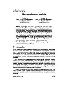
2.2 Data Envelopment Analysis (DEA) Below we briefly discuss DEA, the problem it was developed to address and the basic model it uses. DEA is a linear programming based approach that constructs an efficient frontier (envelopment) over the data, and calculates each data point’s efficiency relative to this frontier (Charnes et al. 1997). DEA assumes that the variables of the data can be logically divided into inputs and outputs. Each data point corresponds to a decision making unit (DMU) in practice. The “decision” of a unit is to convert inputs into outputs as efficient as possible. DEA method uses a linear programming approach to identify the efficient DMUs, those units that make the most efficient use of inputs to produce outputs. The efficient units consist of a frontier among all DMUs. The efficiencies DMUs are measured by projecting to this frontier. To illustrate the basis idea of DEA, assume eight DMUs are to be evaluated as shown in Table 2.2. Each DMU has one input and one output. A typical DEA model would identify five points (1,2,3,4,7) as efficient points and thus these five points form an efficient frontier as shown in Figure 2.1. Three DMUs (5,6,8) are below the frontier and thus they are inefficient according to DEA. For each inefficient DMU, DEA identifies the sources and the level of inefficiency for each of input and output. The level of inefficiency is determined by comparison to a convex combination of other referent DMUs located on the efficient frontier that either utilize lower level of inputs or produce higher level of outputs. Table 2.2: An example of DEA data with Eight DMUs DMU

1

2

3

4

5

6

7

8

X - Input

1

2

3

4

5

6

7

8

Y - Output

1

3

5

6

3

4

7

6

10

8 7 6 5 4 3 2 1 0

7 4

8

3 6 2

5

1 0

1

2

3

4

5

6

7

8

9

Figure 2.1: An Example of DEA Frontier The DEA model in its original form represented the performance or efficiency of the DMU as the ratio of weighted outputs to weighted inputs (Cooper et al. 1999). Up to date, DEA literature has developed numerous models. Detailed references can be found in Charnes et al. (1997), Cooper et al. (1999), Cooper, Park and Yu (1999), Sueyoshi (1999) and Coelli (1996). Essentially, various models for DEA seek to establish which subset of DMUs determines an envelopment surface and characterize each DMU by an efficiency score. One of the classic model formulations, the BCC input-oriented model named after Banker, Charnes and Cooper (1984), is presented as follows: Suppose N data points (DMUs) are to be evaluated. Each data point is consisted of K inputs and M outputs. The K × N input matrix, X, and the M × N output matrix, Y, represent the data consisted of N DMUs. Note that in this formulation, the columns represent the data points and the rows are the variables. Hence for the ith DMU the inputs are represented by the K × 1 vector xi and the outputs by the M × 1 vector yi respectively. A good account of the BCC model can be found in Banker et al. (1984) and Charnes et al. (1997). We directly present its formulation below: min θ λ ,θ

S.t.

-yi + Y λ ≥ 0 ,

θxi - Xλ ≥ 0 , 1′ λ =1,

λ >0,

(1)

11

Where 1 is an N × 1 vector of ones, θ is a scalar and λ is an N × 1 vector of constants. In the BCC model formation, θ and λ are the only two variables to be optimized. All the other values (X, Y) are given by the data. What this linear programming does is essentially identifying a convex hull for all the data points and computing an efficiency score θ for each individual data point. The value of θ is bounded between 0 and 1, with 1 indicating a point on the frontier. Note that the linear programming problem must be solved N times, once for each DMU in the sample. DEA has been applied to study the efficiency of commercial banks (Seiford and Zhu 1999, Soterious and Zenios 1999), to anticipate the consequences of school reforms (Grosskopf et al. 1999) and to investigate online customers shopping efficiency (Xue and Harker 2002). This paper represents the first attempt to apply DEA to study model efficiency and model combination.

3. Equivalence of the DEA and ROC Convex Hulls Both ROCCH and DEA identify a convex hull. In this section we show that the two convex hulls indeed are identical for a 2-class classification problem. We first present some preliminaries. Consider the standard learning problem. A learning algorithm is given training examples of the form (x, y) for some unknown function y = f(x). In this paper, we restrict our attention to discrete y values, that is, we focus on classification problems and the models considered here are classifiers. The y values are drawn typically from a discrete set of classes C ∈ (1, ..., K). Given a set of training examples, a learning algorithm outputs a classifier. The classifier is a hypothesis about the true function f. When there exists a set of models, f1, f2 , …, fm, a model combination method h is a super model in the form of y = h(f1(x) , f2 (x), …, fm (x)).

3.1 ROC Convex Hull Algorithm ROC Convex Hull (Provost and Fawcett 2001) has several distinct characteristics: 1. It is 2-dimensional, characterized by TP and FP of a classifier.

12

2. It goes through (0,0) and (1,1)1, and both TP and FP values are bounded within (0,1). 3. It identifies the convex hull in the northwest area, i.e. above the line TP = FP. 4. It is monotonic and increasing. Two-dimensional convex hull algorithms are essentially variants of the “triangle test”: for a data point to be on the convex hull, it must not be within the triangle formed by any three data points (Barber et al. 1996). But the computation complexity for this test is O(N4) for N records. ROCCH uses an algorithm similar to the Quickhull algorithm (Provost and Fawcett 2001, Barber et al. 1996), the complexity of which is reduced to O(N logN). The property of monotonicity further simplifies the core of the algorithm as follows: “Assume (Xj ,Yj) and (Xj+1 ,Yj+1) are two adjacent points on the current identified convex hull. To evaluate a particular data point (xi, yi) where Xj ≤ xi ≤ Xj+1, we only need to check if (xi,yi) is below or above the line formed by (Xj ,Yj) and (Xj+1 ,Yj+1). If (xi,yi) is below the line, maintain the old convex hull and check new data points. Otherwise, modify the old convex hull to include this new point”2.

3.2 DEA Convex Hull It is not immediately clear how to represent an ROC problem by a DEA model. Here we take the approach that a classifier can be considered as a DMU that makes tradeoffs between TP and FP. A classifier can be perceived as a decision maker that attempts to maximize the output, TP, at the expense of the input, FP. Thus the ROC problem can be formulated into a DEA problem. Definition 1 A 2-class classifier {f(x, y), y ∈ (0,1)} is a DMU in DEA that takes FP as inputs and TP as outputs. We choose the classic BCC formulation (Banker, Charnes and Cooper 1984) here. As mentioned before, note that the formulation below has to be solved for each classifier separately to get its efficiency score. Among a set of M classifiers for evaluating a particular classifier i (with FP=xi and TP=yi) the one-input one-output BCC model simplifies as:

1

i.e. when a naïve model classifies all instances as negative or positive respectively. This is a literal summarization by authors on Fawcett’s Perl script publicly available at http://www.hpl.hp.com/personal/Tom_Fawcett/ROCCH .

2

13

min θ λ ,θ

s.t.

M

∑λ j =1

j

y j ≥ yi

M

∑λ x j =1

j

M

∑λ j =1

j

j

≤ θxi

=1

λj >0

(2)

According to Charnes et al. (1997), the ith DMU is to be on the efficiency frontier, if and only if the solution θ is equal to 1. Thus in order to test whether ROCCH identifies the same convex hull, we just need to prove one of the following two cases: 1.

A model is on the convex hull from ROCCH if and only if it has the property θ =1 in the DEA model.

2.

A model is not on the convex hull from ROCCH if and only if it has the property θ