Benefit-Cost Analysis Using Data Envelopment Analysis

N. K. Womer1, M.-L. Bougnol2, J. H. Dula´1, and D. Retzlaff-Roberts3 1

Hearin Center for Enterprise Science University of Mississippi 2

Haworth College of Business Western Michigan University

3

Mitchell College of Business University of South Alabama

*This work was funded by grant N00014-99-1-0719 from the Office of Naval Research. Corresponding Author:

N. K. Womer Hearin Center for Enterprise Science University of Mississippi University, MS 38677 [email protected] (662) 915 5497

Benefit-Cost Analysis using Data Envelopment Analysis Abstract Benefit-cost analysis is required by law and regulation throughout the federal government. Robert Dorfman (1996) declares “Three prominent shortcomings of benefit-cost analysis as currently practiced are (1) it does not identify the population segments that the proposed measure benefits or harms (2) it attempts to reduce all comparisons to a single dimension, generally dollars and cents and (3) it conceals the degree of inaccuracy or uncertainty in its estimates.” The paper develops an approach for conducting benefit-cost analysis derived from data envelopment analysis (DEA) that overcomes each of Dorfman’s objections. The models and methodology proposed will give decision makers a tool for evaluating alternative policies and projects where there are multiple constituencies who may have conflicting perspectives. This method incorporates multiple incommensurate attributes while allowing for measures of uncertainty. An application is used to illustrate the method.

Key Words (Benefit-cost analysis, data envelopment analysis)

2

Introduction Benefit-cost analysis is required by law and regulation throughout the federal government to decide among alternative policies and projects. It has been recently required in federal regulations designed to protect human health, safety, or the environment. Benefit-cost analysis (BCA) is a practical way of assessing the usefulness of projects, both public and private. It has been extensively applied to projects in defense, transportation, irrigation, waterways, and housing. This technique or variations of it are also referred to cost-effectiveness analysis, cost-benefit analysis, systems analysis, or merely analysis. BCA is the process of using theory, data and models to examine a problem's relevant objectives and alternative means of achieving them. It is used to compare the costs, benefits, and risks of alternative solutions to a problem and to assist decision makers in choosing among them. The history of the subject can be traced to Dupuit's classic 1844 paper "On the Measurement of the Utility of Public Works." The technique has been a mainstay of the Army Corps of Engineers since 1902. Despite its long standing and widespread use, benefit-cost analysis is subject to criticism. Robert Dorfman (1996) declares “Three prominent shortcomings of benefit-cost analysis as currently practiced are (1) it does not identify the population segments that the proposed measure benefits or harms, (2) it attempts to reduce all comparisons to a single dimension, generally dollars and cents, and (3) it conceals the degree of inaccuracy or uncertainty in its estimates.” In part due to criticism like this numerous approaches to decision-making using variants of benefit-cost analysis have evolved. Among them Smith (1986) lists risk-risk analysis, cost effectiveness analysis, risk-benefit analysis, environmental impact statements, and economic impact analysis. This research develops models for conducting benefit-cost analysis based on data envelopment analysis (DEA). Our goal is to provide a tool that can unify this array of techniques by overcoming each of Dorfman’s objections to the current practice of benefit-cost analysis. The DEA model presented gives decision makers a tool for evaluating alternative policies and projects where constituencies may have conflicting perspectives. It also incorporates multiple incommensurate attributes, while allowing for measures of uncertainty.

3

Data Envelopment Analysis While Data Envelopment Analysis (DEA) is typically considered a nonparametric method for comparing efficiency among a set of operating units, it can be adapted to compare alternative policies and projects. In the traditional DEA framework, a group of “decision-making units” (DMUs) are compared to evaluate their relative efficiencies. Each DMU, j, is described by a vector of outputs yj and a vector of inputs xj. For application to benefit-cost analysis the alternatives being compared form the DMUs, costs are analogous to inputs, and benefits are analogous to outputs. In principle, DEA may be applied to any set of DMUs, but the technique is particularly useful when the inputs and outputs are not associated with a known set of market prices that are common to all DMUs. The logic of traditional DEA is straightforward. Efficiency is calculated using a weighted sum of outputs and inputs for each of the entities in the study. The problem is the choice of weights vectors, v and u, to assign to the inputs and outputs respectively. A fixed set of weights that is imposed a priori provokes one of Dorfman's specific criticisms about benefit-cost analyses, reducing benefit-cost measures to a single dollars-and-cents measure that requires determining the monetary value of each attribute. Dorfman (1996, p.3) states “Basically, this mandate would require answers to such questions as ‘What is the value of a human life?’ and ‘How much is an endangered species worth?’” Within the DEA framework, the analyst does not need to answer these questions directly. Rather than requiring such values to be chosen a priori, DEA places few restrictions on the values of inputs and outputs. In a sense, each alternative (each DMU) custom selects its own weights so that that alternative is portrayed in the most favorable light. The result is a classification of each of the alternatives as either “efficient” or “inefficient” relative to the data set. An alternative is efficient if its data point is located on the efficient frontier of a production possibility set characterized by the entire set of all alternatives that are under consideration. Thus, DEA offers a well-defined, nonparametric, procedure for classification of individual alternatives defined by multiple quantitative attributes using an efficiency measure based on weighted sums of outputs and the inputs.

4

The first DEA model by Charnes, et al. (1978) defined efficiency as a ratio of weighted outputs to weighted inputs. The weights are individually and optimally determined for each of the alternatives by solving an optimization problem for each alternative. This optimization problem can be transformed into a linear program (LP) which makes it practical for analyses and decision making. The DEA LP provides a flexible framework for a wide range of efficiency assessment models. In Banker et al. (1989) new LP formulations were introduced to deal with variable, increasing, and decreasing returns to scale DEA models. All these were still based on efficiency definitions based on ratios. Benefit-cost ratios have also been traditional. However, Dorfman (1996, p. 6) is concerned about this as well. “Generally speaking, the ratio of benefits to costs does not measure contribution to social welfare; the excess of benefits over costs does.” Another important DEA model, and one of special interest in this paper, is the “additive” model first introduced by Charnes et al. (1985). Its constant returns to scale formulation is: Max u’y0 - v’x0 u,v,

s.t.

u’Y - v’X u v

≤ 0 ≥ 1 ≥ 1,

(1)

where Y={yj} and X={xj}, and (x0, y0) is the vector of the values of the alternative (one of the j’s) being evaluated. The vectors u and v are the weights or multipliers assigned to this evaluation. The efficiency classification of alternative (x0, y0) using LP (1) is the same as that obtained using an input or output oriented LP formulation if the data and the returns to scales assumptions are the same. What is important about the model used in (1) is that efficiency is evaluated as the difference between the weighted sum of the outputs and the inputs, the ‘excess of benefits over costs” that Dorfman desires. Deriving a Linear Economic Model for BCA The additive constant returns to scale DEA model is the platform on which we construct a new framework for BCA that addresses Dorfman’s concerns about the traditional approach. The first step is to establish its equivalence for BCA analysis. This follows immediately when we treat BCA alternatives as

5

DEA entities. DEA entities are defined by a vector of attribute values. These attributes are either inputs or outputs in the transformation process in which all entities are involved. In the same way, alternatives in a BCA study are the entities and each alternative has multiple costs and benefits. Our DEA model will classify alternatives into efficient or “dominating” alternatives and the rest. The dominating alternatives are those in a frontier of a domination set which is exactly analogous to the DEA constant returns to scale production possibility set. This alone permits the use of a nonparametric frontier analysis to analyze projects for a BCA analysis. This new procedure based on nonparametric frontiers generates a set of dominating alternatives with cardinality at least one. This set necessarily includes any alternative which would have emerged as winner using the traditional approach of an a priori weight assignment. But, the price we pay for the flexibility in weight assignment provided by DEA-type methods is the emergence of possibly many winning projects. We will now begin to modify the model in (1) to address Dorfman’s specific concerns. As with DEA, the set of common attributes that characterize each alternative need to be classified as either costs or benefits. When there are multiple constituencies, what is a valuable benefit to one group may be negligible or even a cost to another group. For example, suppose an alternative under consideration would increase the population of an endangered species such as a wolf. The increased population in the endangered wolf species would be viewed as a positive by environmentalists, but could well be viewed as a negative by those who live and raise livestock in the affected area. To address the dissonant views of the different constituencies, we relax the requirement that any particular attribute needs to be declared a cost or a benefit in advance of the analysis. This is a significant modification from DEA where each attribute is either an input or output and we do not have different constituencies with conflicting views. This permits the analyst to consider the impact of alternatives on constituents who hold relatively different values from the population as a whole. The presence of dissonant constituencies with different perceptions about the role of attributes in the projects of a BCA analysis presents an interesting challenge. Our solution is to relax the restrictions on the multipliers in (1) associated with attributes for which there is no clear classification as cost or

6

benefit. To illustrate the effect of this, consider attribute i which for some it is desirable and for others quite the contrary. The value for this attribute ranges from relatively low to relatively high as we look at all the projects. If this attribute is arbitrarily classified as a benefit then, under model (1), projects where this value is high are likely to dominate while projects where attribute j is low will dominate only if values of the other attributes compensate for j. Allowing weights to be unrestricted means that projects where j is relatively low also have an advantage since a negative weight at this coordinate benefits them more than it does others. Therefore, allowing weights to be unrestricted creates possibilities for additional projects to emerge as dominant since values at not just one but either extreme of the spectrum are favored. Allowing weights to be unrestricted in a model such as (1) means that we change the shape of the production possibility set and the efficient frontier. The production possibility set in DEA is a cone that “envelops” the data defined by the all data points and m positive or negative unit directions, where

m is the number of attributes for each DMU. The unit direction of recession will be positive or negative depending on whether the coordinate is associated with an input (cost) or output (benefit). If the multiplier for a particular coordinate is unrestricted, the production possibility set is modified in that it no longer includes the corresponding unit direction of that coordinate in its definition. If all coordinates have unrestricted weights, this defines a production possibility set which will be the cone of the data alone. The resultant nonparametric model generates a set of dominating DMUs (projects) that is a superset of that obtained when all the weights are restricted. The new approach to the issue of cost, benefits, and the views taken by different constituencies about these is to use restrictions on the weights to determine the classification of an attribute. Attributes which are uncontested as benefits by all constituencies will have non-negative weights. Conversely, attribute values that are generally considered costs will be restricted to be non-positive. Finally, attribute values that are either costs or benefits depending on the constituency will be allowed to have weights take on positive or negative values. This new model allows us to exert a new measure of control by limiting how large positive or negative magnitudes can be in an attempt to model the importance and the impact of the different constituencies.

7

The new formulation for BCA to admit dissonant constituencies is modified as follows Combine the attributes into a single attribute vector wj, and permit some weights to take on a range of real numbers that may include negative values. The elements of wj are defined so that benefits (in the view of most constituents) are made positive values, and inputs or costs are negative values. By allowing some weights to be less restricted, constituencies with views opposite to those of the majority can be accounted for via negative weights. Let W = {wj}. Then the efficiency problem for alternative i is: Max p’w0 p s.t. p’W < 0

(2)

A normalization constraint is required to prevent the trivial solution of p = 0. If an attribute is common to all alternatives and that attribute is uncontested, then it could serve as the normalization rule, for example; pi = 1.

(3)

The choice of one attribute as a numeraire has the advantage of making the weights from all of the linear programming problems comparable to each other, thus simplifying the use of judgment in evaluating efficient DMUs. Alternatively, constraining the weights’ absolute values to add to 1 has the weights measure the relative importance of each attribute. If the weights are regarded as prices and restricted to be non-negative then problem (2) is familiar to the economist. (See Dorfman, Samuelson and Solow (1958, Chapter 13).) This approach is similar to that of Lancaster (1968, Section 9.4) as modified by Womer (1973). It is further developed in Womer et al (2003). If the multipliers are interpreted as prices, the problem searches for the set of prices (for outputs and inputs) that make DMUi as profitable as possible. The constraints on the problem require that these prices be consistent with a competitive equilibrium (no DMU makes economic profits). Alternative normalization constraints define different numeraires for the general equilibrium. Any efficient DMU will have a maximum economic profit of zero. At the associated equilibrium set of prices that DMU is portrayed as a viable competitive firm. If a DMU is not efficient, then there exists no set of equilibrium prices at which the DMU would be a viable competitive firm in the presence of the others.

8

Furthermore, the set of prices calculated when an inefficient DMU is evaluated gives its minimum loss in its most favorable competitive equilibrium. The equilibrium price perspective is also helpful in choosing among the efficient alternatives. The concept of assurance regions is useful for this purpose. Ideas for controlling the range of values for the multipliers or prices have been extensively investigated in DEA. They are explored by Banker and Morey (1989), by Dryson and Thanassoulis (1988), and by Roll, Cook and Golany (1991). These ideas form the logic behind the assurance region notion proposed by Thompson, et al. (1986). Thanassoulis and Allen (1998) interpret the constraints that generate the assurance regions not as restrictions on prices but as unobserved DMUs. Thrall (1995) recommends that the solution to these problems “. . . involves value judgments in which it is desirable to incorporate user knowledge and preferences rather than for the modeler to act alone.” The linear economic model has a unique advantage in forming assurance regions because the prices are comparable across the linear programs. Therefore, the decision-maker can easily incorporate the assurance region bounds as additional constraints on the problems. The requirement that we apply benefit-cost analysis to a wide range of alternatives means that we must address the range of values for the weights that a “reasonable” decision-maker would place on the inputs and outputs. Thus our linear economic model is: Max p’w0 p s.t. p’W < pi = p < p >

0 1 a b

(4)

Here a is the vector of upper bounds placed on the weights and b is the vector of lower bounds, which may include negative values. A particular attribute, i, that is present for all alternatives would be chosen for the normalization constraint. Overcoming Shortcomings of Benefit-cost Analysis Our linear economic model for BCA which is derived from DEA, can be used to overcome the three shortcomings raised by Dorfman. Recall these shortcomings are: (1) it does not identify the population segments that the proposed measure benefits or harms; (2) it attempts to reduce all

9

comparisons to a single dimension, generally dollars and cents; and (3) it conceals the degree of inaccuracy or uncertainty in its estimates.

1. Population Segments Model (4) can be used to recognize the various population segments and incorporate their potentially conflicting view points by allowing attributes to be either positives (benefits) or negatives (costs). For such an attribute the upper bound on the price would be positive and the lower bound would be negative, thus allowing the attribute to be treated in either way. 2. Single Dimension When model (4) is solved for a particular alternative the objective function value will indeed yield a single value which will determine whether the alternative can be efficient at a corresponding feasible price vector. In general though there will be a different price vector associated with each alternative. In the application to follow, we compare all efficient alternatives using each other’s efficient price vectors. This will evaluate the robustness of the efficiency of each alternative using a range of price vectors that would be favored by different constituencies, thus producing several dimensions along which to evaluate the alternatives. 3. Uncertainty Dorfman’s concern about the inaccuracy and uncertainty of estimates in benefit-cost analysis is important and there is no doubt that measuring uncertainty of the cost and benefit estimates is difficult. On the other hand, once measured, Caporaletti, Dula′ and Womer (1999) have shown how to incorporate measures of uncertainty into the DEA framework. In their approach, measures of uncertainty (the variance of construction cost for example) are regarded as additional attributes to be priced along with the others. Thus the value of the alternative is a linear combination of expected values and variances of costs and benefits. The idea that worth is measured as a linear function of expected value and variance is certainly not new. For example this is the basis of the capital asset pricing model that has been popular for years in the finance literature.

10

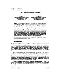
Application To illustrate our method we utilize a real example of a public project where many alternatives were considered, where constituents differed in opinion of which attributes are important, and where some attributes were considered positives by some groups and negatives by other. This example involves the construction of Interstate 40 through Memphis, Tennessee. This highly controversial case went as far as the U.S. Supreme Court, with the controversy stemming from objections to the roadway passing through Overton Park. Interstate 40 through Memphis In 1955 plans were approved to build 68 miles of interstate in and around Memphis Tennessee. The main route of the interstate was planned to pass straight through the city with a by-pass to circle the periphery as shown in Figure 1. Plans included I-40 passing through Overton Park at grade level, taking 26 of the park’s 342 acres. After plans were made public, Memphis citizens who lived in the vicinity of the park began to protest. Alternate routes were proposed and studied but the park route remained recommended due to the large number of homes, businesses, churches, and schools that would have to be destroyed by any other route. In 1966 the DOT Act was passed, containing Section 4(f) that states federal money cannot pay for roads through parks unless no other “feasible or prudent alternative exists.” In late 1969 legal action began to attempt to stop I-40 from passing through Overton Park with Section 4(f) as the basis, with the case reaching the U.S. Supreme Court in late 1970. The Supreme Court ordered an abrupt halt to construction while the case was in progress. Ultimately the Supreme Court did not make a final decision and the case was remanded back to the Secretary of Transportation in 1972 to determine whether or not construction plans were in compliance with Section 4(f). Throughout the 1970’s the Tennessee Department of Transportation (TDOT) continued to study alternatives which included tunneling under the park, elevating a bridge above the park, and many others. With each study the park route continued to be the leading candidate due to the lack of satisfactory alternatives. With the completion of each new study, TDOT sought approval from the Secretary of Transportation but approval was denied each time.

11

The stalemate finally ended in 1981 when the City of Memphis requested to remove the park segment of I-40 from the interstate system, and instead receive substitute funds equal to the cost of the removed project under the “Interstate Substitution Program” that was available at that time. A bored tunnel was the most expensive alternative that had been considered, and the City received $280 million based on the tunnel’s estimated cost. When the Supreme Court halted work in 1970, interstate construction had progressed to what is shown in Figure 2, which is what still exists today. The unfinished I-40 segment east of the Park (inside the I-240 loop) is officially no longer part of the interstate system, and is called Sam Cooper Boulevard. The northern leg of I-240 was deemed to be I-40 as well, adding approximately 6 minutes to the trip through Memphis when there are no traffic delays. No upgrades were made to the two I-40/240 interchanges after I-40 construction was halted, despite the fact that the interchanges were designed to handle only the moderate amount of “bypass” traffic. As a result the two interchanges are frequently the sites of congestion, delays, and accidents involving death and injuries. Other disadvantages include diminished accessibility of downtown Memphis from the eastern part of the city and county. Many believe this has slowed the economic development of downtown Memphis. However, there are also some advantages to the scenario that transpired. Midtown neighborhoods and Overton Park have remained intact, and Overton Park has undergone major improvements. New parks and recreation facilities were acquired with $2.2 million that the city was paid for the 26 acres of park right-of-way in 1969, and the $280 million in substitute funds has been used for local road and transit improvements. Alternatives and Attributes As mentioned above, many alternatives were considered over the years of the I-40/Overton Park saga. For our study, we analyzed the 26 alternatives shown in Table 1. The appendix contains descriptions of the alternatives. Alternatives 1 through 12 involve I-40 passing through the city and were considered by TDOT at various times over the years. Alternatives 19 through 26 involve obtaining the substitute funds, with alternative 23 being what actually happened.

12

Table 1 quantifies the attributes of the alternatives where higher is preferable (for most constituencies) for each attribute. In this manner positive attributes receive positive values while negative attributes receive negative values. As stated earlier, allowing negative prices will incorporate opposing views of other constituencies. The column labeled Park quantifies the impact of each alternative to the park on a scale of 0 to 5, with higher being better for the park. Alternatives that do not affect the park receive a score of 5, with alternative 1 being the worst for the park and receiving a score of 0. The Midtown East and Midtown West variables are binary measures reflecting whether the roadway bisects the area or not. Alternatives which do not bisect the areas are given a score of 1. Time is the additional travel time between the two I40/I240 interchanges, beyond the travel time required for the original plan. So this is 0 for alternatives 1 to 12 and -6 minutes for going around on I-240 with upgraded interchanges, and -15 minutes for using I-240 with base interchanges. The Accidents column measures the additional number of accidents that would be expected in the Memphis area beyond the base case of the original plan. So 0 for alternatives 1 to 12 does not mean there would be 0 accidents, but the values for alternatives 13 to 26 are estimates of the additional accidents resulting from I-40 not being completed as planned, and are shown negatively since more accidents would be worse. These are projections for the year 2000 made by TDOT during the 1970’s. The Work Trip column measures time saved by local commuters by having some form of Sam Cooper Boulevard, so this applies only to those alternatives where I-40 goes around the city with I-240. A partial Sam Cooper (as shown in Figure 2) is estimated to save 2 minutes in commuting time and a full Sam Cooper (extending all the way to Overton Park) is estimated to save 5 minutes in commuting time. Funding reflects whether or not the $280 million in substitute funding for building local roads is obtained, and is shown negatively because higher cost would be worse for the U.S taxpayer. However, this is an attribute that would be considered a positive by some constituents, as will be discussed subsequently. The Overall Cost column shows construction costs as deviations from what was actually built. So alternatives 13 and 24 show costs of $0, more expensive alternatives show a negative cost and less expensive alternatives have positive values. We use the negative of the absolute value of Overall Cost to

13

estimate the variance as based on Caporaletti et al. (1999). The final column of Table 1 is labeled Base. The value of 1 in that column stands for all of the attributes that are shared by all of the alternatives. Without it we would have the impression that the original proposal had no benefits or costs at all. This is surely not the case and the base attribute represents those benefits and costs.

Constituencies There are a number of constituencies with conflicting perspectives on this issue. First there are midtown residents who live near Overton Park who want neither their neighborhood nor the park bisected. Next, there are residents of other parts of Memphis area who want convenient access to downtown and midtown Memphis. The largest constituency is the American public that uses the Interstate system and wants to be able to pass through Memphis on I-40 safely and without delay. Then we have the government (and in turn taxpayers) who want to spend as little as possible to get the highway built. Another constituency would be construction companies who want as much construction as possible to enhance their income. There are also automobile body shops whose income comes primarily from repairing cars damaged in accidents. So, while it may seem morbid to say there is a constituency that views accidents positively, body shops and towing companies would have good reason for this perspective. Thus we have a number of different constituencies with conflicting priorities and different views of the costs and benefits of the available alternatives.

BCA Analysis This Interstate 40 example is used to illustrate the application of our model for selection of alternatives for government projects with multiple constituencies. While the decision has already been made for this example, it provides a good example of a government project in which there are many alternatives and there are also multiple constituencies with conflicting views. This approach to BCA would have been useful had it been applied to a situation such as this. This data set also provides a good example of the type of data that would typically be involved in a BCA analysis for a government project. Unlike a typical DEA analysis where data is collected after the fact, BCA must rely on estimates

14

of costs and benefits that would expected for each alternative, if that alternative were implemented. Typically there will be attributes such as estimated construction cost as well as various environmental impacts. For our analysis the normalization constraint chosen based on (3) is to constrain the price for Overall Cost to be 1. Since Overall Cost is measured in millions of dollars, this defines the units of the other prices in millions of dollars. For example, if the price for accidents were 0.1, then an accident would be valued at $100,000. We also impose constraints on the prices that are used to evaluate project attributes, which are shown at the top of Table 2. The bounds placed on the price of each attribute are intended to estimate of the widest range of values that a decision-maker would place on each price. This has the effect of ignoring some of the constituencies that have been identified but it does not require that only one of the constituencies be selected. For this example, two of the prices (for Accidents and Funding) were permitted to be either positive or negative. Allowing a negative price for Accidents would permit the perspective of body shops and towing companies who would benefit from increased numbers of accidents. Allowing a negative price for Funding reflects the perspective of construction companies and Memphis residents who would be in favor of additional construction funding for the Memphis area. As can be seen in Table 1, Funding was treated as a negative so a positive price shows the perspective of tax payers and the government who want as to spend as little as possible for road construction in Memphis. Preliminary Analysis The preliminary analysis does not adopt the perspective any particular constituency but instead uses the price constraints shown in Table 2 which allows for the views of many constituents. Results show that with such liberal constraints, 14 of the original 26 alternatives are efficient at some set of prices. The other 12 are inefficient and can be excluded from further consideration. Thus this preliminary analysis with minimal restrictions on price is still sufficient to eliminate almost half of the alternatives.

15

The efficient prices are reported in Table 2 for each of the 14 efficient alternatives. This shows the wide range of values that are assigned to attributes in order for some of the alternatives to be efficient. For example, several of the alternatives have the price of Funding at its lower bound of -1 when they are efficient. These would be the alternatives favored by construction companies and Memphis residents. When each of these price vectors is used to evaluate all 14 of the efficient alternatives, typically several of the alternatives are efficient. It is also found that each of the efficient alternatives is efficient at a wide range of prices. Figure 3. illustrates these prices by showing the magnitudes of the values. It provides graphic evidence of some of the vast differences in values that are associated with selecting some of the projects. The attributes are weighted by the prices in Figure 4. For each efficient alternative the attributes that are regarded as positive are exactly offset by attributes that are regarded as negative, as is required by the model. The importance of the various attributes varies dramatically among the efficient projects though. Thus alternative 11 (the southern route) becomes efficient by balancing the negative effects of Overall Cost with the positive effects of the Base and the impact on the Park while ignoring other attributes. In contrast, alternative 13 (the “do nothing” alternative) is efficient by ignoring both of these attributes and balancing the negative effect of Accidents with the positive effect of Work Trip. This preliminary analysis, with minimal restrictions on prices, is still sufficient to eliminate 12 of the 26 projects as inefficient. It also shows the need to further restrict the prices if we are to make a decision among the remaining 14 alternatives.

Secondary Analysis A more restrictive set of price bounds is shown at the top of Table 3. These are the bounds used in the secondary analysis of the remaining 14 alternatives. These restrictions might reflect the preferences of a federal official who sees Overall Cost and Funding as clear measurable negatives but who is less clear about the relative values to attach to other attributes of the projects. We evaluate each option under the price constraints.

16

Results show that five of them are efficient at some set of prices. These five and are shown in Table 3 along with their respective efficient price vectors. The other alternatives cannot be efficient under these restrictions, so we abandon them and continue to compare the remaining five. The effect of these restrictions is illustrated in Figure 5, which shows the value placed on each attribute for each alternative. Some of the attributes are not valued in any of the price sets. It seems clear from Figure 5 that Overall Cost, Accidents, the Base, and the Park dominate the tradeoffs that make these alternatives efficient. To help us choose among these projects we use Figure 6 to evaluate each of the five projects at the five price vectors. Figure 6. shows the cross efficiencies of Sexton et al (1986) and Doyle and Green (1994) that correspond to our linear model for the five alternatives. Each of the other alternatives is inefficient when evaluated at the prices that make 240D efficient. On the other hand 240D is efficient not only at its own prices but also at the prices that make each of the others efficient. Of course one reason that 240D is efficient is that neither Time (which reflects increased travel time through Memphis) nor Work Trip are considered valuable for any of these price vectors, and 240D is the worst alternative for both of these attributes. Consequently alternative 240D is not penalized for having inflated travel time that would result from traffic congestion. Other sets of restrictions that forced value to be associated with increased travel time would yield other results. Even so, this analysis could serve as the motivation to further investigate the desirability of the 240D and the consideration of further price restrictions that could ultimately identify the preferred alternative. Conclusion This paper has illustrated the use of a linear economic model derived from DEA as a means of performing benefit-cost analysis that is required by law and regulation for many public projects. The application of our method to a real example of a controversial public project illustrates the potential benefits. While the decision was previously made for this Interstate 40 through Memphis example, it provides a good example of a public project with many alternatives and multiple constituencies with conflicting perspectives. This data set is very representative of the type of data that would typically be involved in conducting BCA, where costs and benefits must be estimated prior to implementation of any of the alternatives.

17

Our proposed methodology overcomes each the shortcomings of BCA as identified by Dorfman. This approach permits each constituency to express values about important attributes that reflect their perspective. By analyzing the choice among attributes subject to the constituencies’ restrictions on prices, we can gage the extent to which each choice would help or harm that constituency. Data envelopment analysis is at its heart a problem in vector maximization, which involves more than one value. In addition, our approach of evaluating all efficient alternatives with all efficient price vectors provides a multifaceted analysis and identifies those alternatives that are most robust in efficiency. Therefore this approach to BCA deals effectively with the problem of reducing the problem to a single value. Our approach also can include measures of uncertainty in the form of the variance of benefits or costs and in that way deals with the uncertainties that are inherent in new public projects. References Banker, R., A. Charnes, W.W. Cooper, J. Swarts, and D. A. Thomas, 1989. "An Introduction to Data Envelopment Analysis with Some of its Models and Their Uses," Research in Governmental and Nonprofit Accounting 5, JAI Press Inc., Greenwich, CT. Banker, R. and R. Morey. 1989. "Incorporating Value Judgments in Efficiency Analysis," Research in Governmental and Nonprofit Accounting 5, JAI Press Inc., Greenwich, CT. Caporaletti, L., J. H. Dulá, and N. K. Womer, 1999. “Performance Evaluation Based on Multiple Attributes with Nonparametric Frontiers,” Omega 27, 637-645. Charnes, A., W. W. Cooper, B. Golany, L. Seiford, and J. Stutz, 1985. “Foundations of Data Envelopment Analysis for Pareto-Koopmans Efficient Empirical Production Functions,” Journal of Econometrics 30, 91107. Charnes, A., W. W. Cooper and E. Rhodes, 1978. "Measuring the Efficiency of Decision Making Units," European Journal of Operational Research 1, 429-444. Dorfman R. 1996. “Why Benefit-Cost Analysis Is Widely Disregarded and What to Do about It,” Interfaces 26, 1-6. Dorfman R., P. A. Samuelson, and R. M. Solow, 1958. Linear Programming and Economic Analysis, McGraw-Hill, New York, NY. Doyle, J. R. and R. Green, 1994. “Efficiency and Cross-Efficiency in Data Envelopment Analysis: Derivatives, Meanings and Uses,” Journal of the Operational Research Society 45 No. 5, 567-578. Dryson, R.G. and E. Thanassoulis. 1988. "Reducing Weight Flexibility in Data Envelopment Analysis," Operational Research Society 39, 563-576. Dupuit, J. 1844. De la Mesure de l'utilite' des travaux publics. Reprinted in Jules Dupuit, De l'utilite' et de sa mesure, Torino, la Roforma sociale. 1933.

18

Lancaster, K. 1968. Mathematical Economics, Macmillan. Roll, Y., W. D. Cook, and B. Golany, 1991. "Controlling Factor Weights in Data Envelopment Analysis," IIE Transactions 23, No. 1, 2-9. Sexton, L. M., R. H. Silkman, and A. J. Hogan, 1986. “Data Envelopment Analysis: Critique and Extensions,” In: R. H. Silkman (Ed.) Measuring Efficiency: an Assessment of Data Envelopment Analysis. Jossey-Bass, San Francisco, CA, 73-105. Smith, V. K., 1986. “A Conceptual Overview of the Foundations of Benefit-Cost Analysis.” In Bentkover, Vincent Covello, and Jeryl Mumpower (eds.). Benefits Assessment: The State of the Art. Dordrecht: D.Reidel Publishing Co. Thanassoulis, E. and R. Allen. 1998. “Simulating Weights Restrictions in Data Envelopment Analysis by Means of Unobserved DMUs,” Management Science 44, No. 4, 586-594. Thompson, R. G., F.D. Singleton, R.M. Thrall, and B.A. Smith, 1986. “Comparative Site Evaluations for Locating a High-Energy Physics Lab in Texas,” Interfaces 16, No. 6, 35-49. Thrall, R. M. 1995. “Duality, Classification and Slacks in DEA,” Working Paper No. 121, Rice University. Womer, N. K. 1973. “Lancaster’s Version of the Walras-Wald Model,” Journal of Economic Theory 6, No. 5, 515-519. Womer, N. K., H. F. E. Shroff, T. R. Gulledge, and K. E. Haynes, 2003. “Measuring Efficiency with a Linear Economic Model,” forthcoming in Applied Economics. APPENDIX: DESCRIPTION OF ALTERNATIVES Alternatives 1 through 12 involve I-40 passing through central Memphis 1. The Original Plan from 1955 was to bisect the Park at grade. This would have been the worst alternative for the quality of the Park. The Park would have been divided into two separate parts with limited access between. The roadway would have been a visual obstruction and brought more air and noise pollution to the Park. 2. The Cut & Cover Alternative is the most inexpensive way of building a tunnel, by digging it from above as an open trench and then covering the top. This would have allowed the Park to be unaffected after construction was complete, but would have been very disruptive during construction. Tunnels in general have the disadvantage of higher maintenance costs due to requiring mechanical ventilation and pumping water to keep the tunnel dry. 3. The Cut & Cover Stacked tunnel would have allowed a narrower strip of land be disturbed, by stacking the two directions of traffic on top of each other. But this would have required digging deeper into the water table and a greater need to pump water. 4. The Bored Tunnel would not have disturbed the Park during construction, but it was extremely expensive. It would also have required ventilation and pumping. Ironically, the

19

fact that this alternative was considered, at an estimated cost of $280 million, was what allowed Memphis to later receive the $280 million in substitute funds. 5. The Partially Depressed roadway is similar to No. 1, but less intrusive visually by lowering the traffic out of the line of sight. It would have avoided the need for mechanical ventilation. But it would still have divided the Park with limited access between. 6. A Bridge Above the Park would have elevated the interstate and been less divisive to the Park than 1 or 5 but would have been unsightly and caused more noise pollution than a tunnel or depressed alternative. It would also have been disruptive during construction. 7. A Fully Depressed roadway with plazas would have many advantages. The plazas would have provided the advantage of the tunnels, allowing good access to both sides of Park. The open sections would have provided the advantage of no. 5, of not requiring mechanical ventilation or pumping. It would have been disruptive during construction. 8. Cut and Cover under North Parkway is similar to No. 2 but the path would have been under North Parkway along the northern edge of the Park, rather than through the middle of the Park. During construction this would disrupt the Park less, but would have been very disruptive to traffic for North Parkway. 9. Elevated Above North Parkway is similar to No.6 but the path would have been similar to No. 8. 10. The northern route would have completely avoided the Park by moving I-40 further north. This would have been advantageous for the Park, but the path was through heavily developed areas and would have required relocating many more homes, businesses, churches, and schools. 11. The southern route is similar to the northern route but would have passed to the south of the Park with the same advantages and disadvantages. 12. The L&N route was an old railroad right-of-way but the width was insufficient for the 6 lanes planned for I-40. Alternatives 13 through 18 involve I-40 joining the northern leg of I-240 13. The do nothing alternative is what actually happened (except this alternative does not include the $280 million in substitute funds). This includes an abruptly ending I-40 dumping into a local road. This unfinished segment of I-40 is now called Sam Cooper Blvd. 14. 240A is the same as No. 13 but would have upgraded the two I-40/240 interchanges to handle the volume of traffic from I-40. 15. 240B is the same as No. 13 but would have extended Sam Cooper all the way to East Parkway (the eastern edge of the Park). East Parkway is a major road, which could better handle the traffic, and these additional miles of speedy travel would dramatically improve access between midtown and east Shelby County.

20

16. 240C would combine the upgrades from No. 14 and No. 15, by upgrading the I-40/240 interchanges and extending Sam Cooper to East Parkway. 17. 240D is like No. 13 but completely eliminates Sam Cooper. This alternative spends the least amount money but is the worst possible for accidents and inflated travel time. 18. 240E would omit Sam Cooper, but would upgrade the I-40/240 interchanges to handle the traffic volume from I-40. This would have been the design if I-40 had never been planned to pass straight through Memphis. Alternatives 19 through 26 involve receiving the Federal substitute funds by first planning I-40 through central Memphis and then canceling it. In each one of these I-40 joins the northern leg of I-240. 19. Split and Elevated 1 involves building a local highway split around the Park and elevated. This would provide good local access between downtown, midtown, and east Shelby County. This would also include extending Sam Cooper all the way to the eastern edge of the Park to connect to the elevated roadway. 20. Split and Elevated 2 is the same as 19 but would upgrade the I-40/240 interchanges to handle the volume of I-40 through-traffic. 21. Sam Cooper to Park 1 is the same as what actually happened but extends Sam Cooper to East Parkway. 22. Sam Cooper to Park 2 extends Sam Cooper and also upgrades the I-40/240 interchanges. 23. Actual is what really happened with Sam Cooper abruptly ending and inadequate I-40/240 interchanges. 24. Actual plus Interchanges is the same as No. 23 but with upgraded interchanges. 25. No Sam Cooper 1 is the same as No. 23 but with Sam Cooper completely eliminated. 26. No Sam Cooper 2 is the same as No. 23 but with Sam Cooper completely eliminated, and the interchanges upgraded.

21

As

Planned

M ississippi R iver

I-240 W est I-40/240 Interchange

I-40

O verton Park

E ast I-40/240 Interchange

I-240

I-55

Figure 1

As M is sis s ip p i R iv e r

B u ilt

I-4 0 / I-2 4 0

I-4 0 I-4 0

O v e rto n P a rk

In te rsta te q u a lity Sam C ooper

I-2 4 0

I-5 5

Figure 2

22

Table 1. Data for the Twenty-six Alternatives Alternatives Number

Name

Park

1 2 3 4 5 6 7 8 9 10 11 12 13 14 15 16 17 18 19 20 21 22 23 24 25 26

Original Plan Cut&Cover Cut&Cover Stacked Bored Tunnel Partially Depressed Bridge Above Park Fully Depressed Cut&Cover under N.Pkwy Elevated above N.Pkwy Northern Route Southern Route L&N Route Do Nothing 240A 240B 240C 240D 240E Split & Elevated 1 Split & Elevated 2 S. Cooper To Park 1 S. Cooper To Park 2 Actual Actual + Interchanges No S. Cooper 1 No S. Cooper 2

0 4 4 5 1 3 3 5 5 5 5 5 5 5 5 5 5 5 5 5 5 5 5 5 5 5

Midtown Midtown East West 0 0 0 0 0 0 0 0 0 0 0 1 0 0 0 0 1 1 0 0 0 0 0 0 1 1

0 0 0 0 0 0 0 0 0 0 0 1 1 1 1 1 1 1 0 0 1 1 1 1 1 1

Time (Minute)

Accidents

Work Trip

Funding

Overall Cost

Variance

Base

0 0 0 0 0 0 0 0 0 0 0 0 -15 -6 -15 -6 -15 -6 -15 -6 -15 -6 -15 -6 -15 -6

0 0 0 0 0 0 0 0 0 0 0 0 -1997 -875 -1997 -750 -1997 -1000 -1997 -750 -1997 -750 -1997 -875 -1997 -1000

0 0 0 0 0 0 0 0 0 0 0 0 2 2 5 5 0 0 5 5 5 5 2 2 0 0

0 0 0 0 0 0 0 0 0 0 0 0 0 0 0 0 0 0 -280 -280 -280 -280 -280 -280 -280 -280

-17.0 -85.1 -107.5 -280.0 -16.4 -21.2 -25.9 -157.5 -29.8 -31.0 -26.0 -40.0 0.0 -34.0 -9.8 -43.8 38.8 4.8 -28.2 -62.2 -9.8 -43.8 0.0 -34.0 38.8 4.8

-17.0 -85.1 -107.5 -280.0 -16.4 -21.2 -25.9 -157.5 -29.8 -31.0 -26.0 -40.0 0.0 -34.0 -9.8 -43.8 -38.8 -4.8 -28.2 -62.2 -9.8 -43.8 0.0 -34.0 -38.8 -4.8

1 1 1 1 1 1 1 1 1 1 1 1 1 1 1 1 1 1 1 1 1 1 1 1 1 1

Table 2. Prices for the Efficient Alternatives in Preliminary Analysis.

Upper Bound Lower Bound

Park 200 0

Midtown Midtown Time Work East West (Minute) Accidents Trip 200 200 200 200 200 0 0 0 -1 0

Funding 1 -1

Overall Cost Variance Base 1 3 200 1 0 0

Park 0 2.4 2.4 5.2 0 0 0 0 0 0 0 0 0 0

Efficient Prices Midtown Midtown Time Work East West (Minute) Accidents Trip 0 0 0 0.34 0.00 0 0 0 0.03 8.43 0 0 0 0.35 0.00 0 14 0 0.37 0.00 0 0 0 0.01 13.07 0 0 0 0.11 51.40 0 0 0 0.03 12.85 0 0 0 0.02 9.72 0 0 0 0.00 0.00 0 0 0 0.02 9.72 0 0 0 0.31 0.00 0 0 0 0.04 13.07 0 0 0 0.02 0.00 0 0 0 0.03 0.00

Funding -1.00 0.00 -1.00 -1.00 0.00 0.00 0.00 0.00 0.00 0.00 -1.00 -0.16 0.00 -0.10

Overall Cost Variance Base 1 0 16.4 1 0 14 1 0 14 1 0 0 1 3 0 1 3 0 1 0 0 1 0 0 1 1 0 1 0 0 1 0 0 1 3 0 1 0 0 1 0 0

Efficient Alternatives Number 5 6 11 12 13 15 16 17 18 21 22 23 25 26

Name Partially Depressed Bridge Above Park Southern Route L&N Route Do Nothing 240B 240C 240D 240E S. Cooper To Park 1 S. Cooper To Park 2 Actual No S. Cooper 1 No S. Cooper 2

24

Figure 3. Prices from Preliminary Analysis 60

50

40 base variance overall cost 30

Funding Work Trip Accidents Time (minute)

20

midtown west midtown east park 10

pa rt ia lly

24 0B

24 0C

24 0D

24 0E

ua l ac t

1 de pr es se d no S. co op er 2 no S. co op er 1 L& N ro ut e do no br th id in ge g ab ov e pa rk

pa rk

2 pa rk

oo pe rt o

S. c

oo pe rt o

-10

S. c

so ut he rn

ro ut e

0

Figure 4. The relative impact of the attributes in analysis one. 60%

40%

base variance

20%

overall cost Funding Work Trip

0%

-40%

-60%

2

24 0B

24 0C

24 0D

24 0E

al ac tu

1 de pr es se d no S. co op er no 2 S. co op er 1 L& N ro ut e do no br th id in ge g ab ov e pa rk

pa rt ia lly

o er t

pa rk

pa rk o oo p

er t S. c

S. c

so u

-20%

oo p

th er n

ro ut

e

2

Accidents Time (minute) midtow n w est midtow n east park

Table 3: Prices for Secondary Analysis

Park Upper Bound 5 Lower Bound 0 Efficient Alternatives Number 5 6 11 17 18

Name Partially Depressed Bridge Above Park Southern Route 240D 240E

Midtown Midtown Time Work Overall East West (Minute) Accidents Trip Funding Cost Variance Base 5 5 5 1 5 1 1 2 20 0 0 0 0.02 0 0.5 1 0 0 Efficient Prices

Park 0 2.4 5 0 5

Midtown Midtown Time Work Overall East West (Minute) Accidents Trip Funding Cost Variance Base 0 0 0 0.03 0 0.5 1 0.00 16.4 0 0 0 0.03 0 0.5 1 0.00 14 0 0 0 0.03 0 0.5 1 0.00 1 0 1.14 0 0.02 0 0.5 1 0.00 0 0 0 0 0.03 0 0.5 1 0.15 0

Figure 5. The relative impact of the attributes in secondary analysis. 60%

40%

base

20%

variance overall cost Funding Work Trip

0% 240E

bridge above park

southern route

partially depressed

240D

Accidents Time (minute) midtown west midtown east

-20%

-40%

-60%

park

Figure 6. The five alternatives each evaluated at all five price vectors. 5

0

240E

Bridge Above Park

Southern Route

Partially Depressed

240D

Efficiency

-5

240E Prices

-10

Bridge Above Park Prices Southern Route Prices Partially Depressed Prices -15

240D Prices

-20

-25

-30

3