Data Envelopment Analysis Data Envelopment Analysis (DEA) is an increasingly popular management tool. DEA is commonly used to evaluate the efficiency of a number of producers. A typical statistical approach is characterized as a central tendency approach and it evaluates producers relative to an average producer. In contrast, DEA compares each producer with only the "best" producers. By the way, in the DEA literature, a producer is usually referred to as a decision making unit or DMU. DEA is not always the right tool for a problem but is appropriate in certain cases. In DEA, there are a number of producers. The production process for each producer is to take a set of inputs and produce a set of outputs. Each producer has a varying level of inputs and gives a varying level of outputs. For instance, consider a set of nursing homes. Each nursing home has a certain number of registered nurses, other health care workers, a certain square footage of space, and a certain number of managers (the inputs). There are a number of measures of the output of nursing homes, for example, different type of patients (the outputs). DEA attempts to determine which of the facilities are most efficient, and to point out specific inefficiencies of the others. A fundamental assumption behind this method is that if a given producer, A, is capable of producing Y(A) units of output with X(A) inputs, then other producers should also be able to do the same if they were to operate efficiently. Similarly, if producer B is capable of producing Y(B) units of output with X(B) inputs, then other producers should also be capable of the same production schedule. Producers A, B, and others can then be combined to form a composite producer with composite inputs and composite outputs. Since this composite producer does not necessarily exist, it is typically called a virtual producer. The heart of the analysis lies in finding the "best" virtual producer for each real producer. If the virtual producer is better than the original producer by either making more output with the same input or making the same output with less input then the original producer is inefficient. The subtleties of DEA are introduced in the various ways that producers A and B can be scaled up or down and combined.
Numerical Example To illustrate how DEA works, let's take an example of three banks. Each bank has exactly 10 tellers (the only input), and we measure a bank based on two outputs: Checks cashed and Loan applications. The data for these banks is as follows:
Bank A: 10 tellers, 1000 checks, 20 loan applications Bank B: 10 tellers, 400 checks, 50 loan applications Bank C: 10 tellers, 200 checks, 150 loan applications
Now, the key to DEA is to determine whether we can create a virtual bank that is better than one or more of the real banks. Any such dominated bank will be an inefficient bank.
Consider trying to create a virtual bank that is better than Bank A. Such a bank would use no more inputs than A (10 tellers), and produce at least as much output (1000 checks and 20 loans). Clearly, no combination of banks B and C can possibly do that. Bank A is therefore deemed to be efficient. Bank C is in the same situation. However, consider bank B. If we take half of Bank A and combine it with half of Bank C, then we create a bank that processes 600 checks and 85 loan applications with just 10 tellers. This dominates B (we would much rather have the virtual bank we created than bank B). Bank B is therefore inefficient. Another way to see this is that we can scale down the inputs to B (the tellers) and still have at least as much output. If we assume (and we do), that inputs are linearly scalable, then we estimate that we can get by with 6.3 tellers. We do that by taking .34 times bank A plus .29 times bank B. The result uses 6.3 tellers and produces at least as much as bank B does. We say that bank B's efficiency rating is .63. Banks A and C have an efficiency rating of 1.
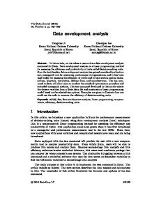
Graphical Example The single input two-output or two input-one output problems are easy to analyze graphically. The previous numerical example is now solved graphically. (An assumption of constant returns to scale is made and explained in detail later.) The analysis of the efficiency for bank B looks like the following:
If it is assumed that convex combinations of banks are allowed, then the line segment connecting banks A and C shows the possibilities of virtual outputs that can be formed from these two banks.
Similar segments can be drawn between A and B along with B and C. Since the segment AC lies beyond the segments AB and BC, this means that a convex combination of A and C will create the most outputs for a given set of inputs. This line is called the efficiency frontier. The efficiency frontier defines the maximum combinations of outputs that can be produced for a given set of inputs. Since bank B lies below the efficiency frontier, it is inefficient. Its efficiency can be determined by comparing it to a virtual bank formed from bank A and bank C. The virtual player, called V, is approximately 54% of bank A and 46% of bank C. The efficiency of bank B is then calculated by finding the fraction of inputs that bank V would need to produce as many outputs as bank B. This is easily calculated by looking at the line from the origin, O, to V. The efficiency of player B is OB/OV which is approximately 63%. This figure also shows that banks A and C are efficient since they lie on the efficiency frontier. In other words, any virtual bank formed for analyzing banks A and C will lie on banks A and C respectively. Therefore since the efficiency is calculated as the ratio of OA/OV or OC/OV, banks A and C will have efficiency scores equal to 1.0. The graphical method is useful in this simple two dimensional example but gets much harder in higher dimensions. The normal method of evaluating the efficiency of bank B is by using a linear programming formulation of DEA. Since this problem uses a constant input value of 10 for all of the banks, it avoids the complications caused by allowing different returns to scale. Returns to scale refers to increasing or decreasing efficiency based on size. For example, a manufacturer can achieve certain economies of scale by producing a thousand circuit boards at a time rather than one at a time - it might be only 100 times as hard as producing one at a time. This is an example of increasing returns to scale (IRS.) On the other hand, the manufacturer might find it more than a trillion times as difficult to produce a trillion circuit boards at a time though because of storage problems and limits on the worldwide copper supply. This range of production illustrates decreasing returns to scale (DRS.) Combining the two extreme ranges would necessitate variable returns to scale (VRS.) Constant Returns to Scale (CRS) means that the producers are able to linearly scale the inputs and outputs without increasing or decreasing efficiency. This is a significant assumption. The assumption of CRS may be valid over limited ranges but its use must be justified. As an aside, CRS tends to lower the efficiency scores while VRS tends to raise efficiency scores.
Using Linear Programming Linear programming (LP) is a mathematical method for determining a way to achieve the best outcome (such as maximizing profit or minimizing cost) in a given math model and a set of requirements represented as linear relationships.
Data Envelopment Analysis is a linear programming procedure for a frontier analysis of inputs and outputs. DEA assigns a score of 1 to a unit only when comparisons with other relevant units do not provide evidence of inefficiency in the use of any input or output. DEA assigns an efficiency score less than one to (relatively) inefficient units. A score less than one means that a linear combination of other units from the sample could produce the same vector of outputs using a smaller vector of inputs. The score reflects the radial distance from the estimated production frontier to the DMU under consideration. There are a number of equivalent formulations for DEA. The most direct formulation of the exposition I gave above is as follows: Let X i be the vector of inputs into DMU i . Let Yi be the corresponding vector of outputs. Let X 0 be the inputs into a DMU for which we want to determine its efficiency and Yi be the outputs. So the X's and the Y's are the data. The measure of efficiency for DMU 0 is given by the following linear program:
Min s.t.
X X Y Y i
i i
i
0
0
i 0
where i is the weight given to DMU i in its efforts to dominate DMU 0 and is the efficiency of DMU 0 . So the ' s and are the variables. Since DMU 0 appears on the left hand side of the equations as well, the optimal cannot possibly be more than 1. When we solve this linear program, we get a number of things: 1. The efficiency of DMU 0 ( ) with 1 meaning that the unit is efficient. 2. The unit's “comparables” (those DMU with nonzero ). 3. The “goal” inputs (the difference between X 0 and i X i ) 4. Alternatively, we can keep inputs fixed and get goal outputs (
1
Y ) i
DEA assumes that the inputs and outputs have been correctly identified. Usually, as the number of inputs and outputs increase, more DMUs tend to get an efficiency rating of 1 as they become
too specialized to be evaluated with respect to other units. On the other hand, if there are too few inputs and outputs, more DMUs tend to be comparable. In any study, it is important to focus on correctly specifying inputs and outputs.
Example: 3 DMU, 2 inputs and 3 outputs Input
Output
DMU 1
5
14
9
4
16
2
8
15
5
7
10
3
7
12
4
8
13
The linear programs for evaluating the 3 DMUs are given by:
LP for evaluating DMU 1: min
LP for evaluating DMU 2: min
LP for evaluating DMU 3: min
st 5L1+8L2+7L3 - 5 = 4 16L1+10L2+13L3 >= 16 L1, L2, L3 >= 0
st 5L1+8L2+7L3 - 8 = 7 16L1+10L2+13L3 >= 10 L1, L2, L3 >= 0
st 5L1+8L2+7L3 - 7 = 9 16L1+10L2+13L3 >= 13 L1, L2, L3 >= 0
SAS program and output
The LP Procedure for DMU 1 Variable Summary Variable Col Name Status Type 1 2 3 4 5 6 7 8 9 10 11
x1 x2 x3 theta const1 const2 const3 const4 const5 const6 const7
12 const8
BASIC
Price
Activity
Reduced Cost
DEGEN DEGEN BASIC DEGEN
NON-NEG NON-NEG NON-NEG NON-NEG SLACK SLACK SURPLUS SURPLUS SURPLUS SURPLUS SURPLUS
0 0 0 1 0 0 0 0 0 0 0
1 0 0 1.0444444 0 0.9555556 1 0 0 0.2 0 0 0 0.1111111 0 0 0 0 1 0 0 0
DEGEN
SURPLUS
0
0
0
Price
Activity
Reduced Cost
0 0 0 1 0 0 0 0 0 0 0
0.2499081 0.0444689 0.6321205 0.753767 0 0 0 0 2.6607865 0.2499081 0.0444689
0 0 0 0 0.0788313 0.0246233 0.0501654 0.0718486 0 0 0
BASIC DEGEN
The LP Procedure for DMU 2 Variable Summary Variable Col Name Status Type 1 2 3 4 5 6 7 8 9 10 11
x1 x2 x3 theta const1 const2 const3 const4 const5 const6 const7
BASIC BASIC BASIC BASIC
BASIC BASIC BASIC
NON-NEG NON-NEG NON-NEG NON-NEG SLACK SLACK SURPLUS SURPLUS SURPLUS SURPLUS SURPLUS
12 const8
BASIC
SURPLUS
0 0.6321205
0
The LP Procedure for DUM3 Variable Summary Variable Col Name Status Type 1 2 3 4 5 6 7 8 9 10 11
x1 x2 x3 theta const1 const2 const3 const4 const5 const6 const7
12 const8
DEGEN DEGEN BASIC BASIC
Price
Activity
Reduced Cost
DEGEN DEGEN
NON-NEG NON-NEG NON-NEG NON-NEG SLACK SLACK SURPLUS SURPLUS SURPLUS SURPLUS SURPLUS
0 0 0 1 0 0 0 0 0 0 0
0 0 0 0 1 0 1 0 0 0.0699677 0 0.0425188 0 0 0 0.040366 0 0.0489774 0 0 0 0
BASIC
SURPLUS
0
1
DEGEN
0
Note that DMUs 1 and 3 are overall efficient and DMU 2 is inefficient with an efficiency rating of 0.753767. Hence the efficient levels of inputs and outputs for DMU 2 are given by:
Efficient levels of Inputs:
5 7 5.67 0.2499081* 0.6321205* 14 12 11.08
Efficient levels of Outputs:
9 4 4.78 0.2499081* 4 0.6321205* 8 6.69 16 13 12.22
Note that the outputs are at least as much as the outputs currently produced by DMU 2 and inputs are at most as big as the 0.753767 times the inputs of DMU 2. This can be used in two different ways: The inefficient DMU should target to cut down inputs to equal at most the efficient levels. Alternatively, an equivalent statement can be made by finding a set of efficient levels of inputs and outputs by dividing the levels obtained by the efficiency of DMU 2. This focus can then be used to set targets primarily for outputs rather than reduction of inputs.
VRS (constant return to scale)
Min s.t.
X X Y Y 1 i
i
i i
0
0
i
i 0 VRS (increasing return to scale)
Min s.t.
X X Y Y 1 i
i
i i
0
0
i
i 0 VRS (non-increasing return to scale)
Min s.t.
X X Y Y 1 i
i i i
i 0
i
0
0
A Real Example
1. Efficient Pricing
Efficiency vs. Direct Cost Cost = 175.75-51.503*Efficiency
300 250
Introduce DEA Daily Rate
200 150 100 50 0 0.1
0.2
0.3
0.4
0.5
0.6
efficieny
2. Explain the distribution above (no consistent pricing) See example of the pricing by size
0.7
0.8
0.9
1
The Factors That Affect Efficiency Statistical Sign + + + + + -
significance1 * *
Bed size dummy 2
-
*
Difficulty index3 Downstate dummy Quality score
+ + -
* *
Private payers as share of total Managed care patients as share of total Facility bed utilization rate Special care patients as share of total Proprietary facility dummy Public facility dummy
* *
1
An asterisk denotes estimate was significant at the 5 percent level.
2
Dummy equals one if number of beds is greater than 300; zero otherwise.
3
Case mix adjusted ouput divided by actual output.