Chapter 2

Data Envelopment Analysis

Technology Analysis of performance has economic production theory as its foundation. Firms employ inputs to produce output typically with an incentive to maximize profits. Firms that are technically inefficient could increase outputs and revenue with the same inputs or could decrease inputs and cost with the same outputs. Farrell (1957) provided a decomposition of inefficiency into technical and allocative parts. From an input-oriented perspective, firms that are not operating on the isoquant associated with observed production are technically inefficient. Farrell provided a comprehensive measure of technical efficiency as the equiproportional reduction of all inputs holding output at current levels. Allocative efficiency is then measured relative to the cost minimizing mix of inputs given observed input prices. Farrell provided the formulation to handle a single output in the case of constant returns to scale. The paper also discussed decreasing returns to scale and the extension to multiple outputs. Farrell and Fieldhouse (1962) extended the approach as a linear program allowing increasing returns to scale. Afriat (1972) provided the formulation for technical efficiency measurement that was consistent with data envelopment analysis (DEA). The theoretical foundations of efficiency measurement are provided in F€are et al. (1994). DEA is the term coined in the operations research literature by Charnes et al. (1978) (CCR) to measure the technical efficiency of a given observed decisionmaking unit (DMU) assuming constant returns to scale. Their linear programming formulation allowed multiple inputs and multiple outputs. Banker et al. (1984) (BCC) extended the CCR model to allow variable returns to scale and showed that solutions to both CCR and BCC allowed a decomposition of CCR efficiency into technical and scale components. In this section, we introduce the representation of the technology that serves as the basis for efficiency measurement. We assume that decision-making units use a vector of m discretionary inputs X ¼ (x1,. . .,xm) to produce a vector of s outputs Y ¼ ( y1,. . .,ys). We represent the individual inputs and outputs of netput ðYj ; Xj Þ for DMUj ( j ¼ 1, . . ., n) as xij(i ¼ 1,. . .,m) and ykj (k ¼ 1,. . .,s), respectively. Following Lovell (1993) we assume that production can be characterized by an input set

J. Ruggiero, Frontiers in Major League Baseball, Sports Economics, Management and Policy 1, DOI 10.1007/978-1-4419-0831-5_2, # Springer Science+Business Media, LLC 2011

7

8

2 Data Envelopment Analysis

LðYÞ ¼ fX : ðY; XÞ is feasibleg:

(2.1)

For each output vector Y we define the isoquant for input set L(Y) as Isoq LðYÞ ¼ fX : X 2 LðYÞ; lX= 2LðYÞ; l 2 ½0; 1Þg:

(2.2)

The isoquant represents the boundary such that the observed production of Y cannot be achieved with any equiproportional reduction in all inputs. The definition of the isoquant for the input set provides the theoretical basis for input-oriented models of technical efficiency. Alternatively, production can be represented by an output set PðXÞ ¼ fY : ðY; XÞ is feasibleg:

(2.3)

Similar to the input set, we define the isoquant for the output set P(X) for each input vector X as Isoq PðXÞ ¼ fY : Y 2 PðXÞ; l1 Y= 2PðXÞ; l 2 ½0; 1Þg:

(2.4)

This isoquant represents the boundary of the output set; without additional resources, equiproportional expansion of all outputs is infeasible. The output set isoquant provides the basis for evaluating technical efficiency in the output-oriented model. To make the connection to the formulation of Banker, Charnes, and Cooper, we define the technology as T ¼ fðX; YÞ : Y 2 PðXÞg ¼ fðX; YÞ : X 2 LðYÞg:

(2.5)

In Sect. 2, the input-oriented models of efficiency are developed; more structure is also placed on the production technology with assumptions on scale economies.

Input-Oriented Models The Farrell (1957) input-oriented measure of technical efficiency of DMUj is given by FðYj ; Xj Þ ¼ minfl : lXj 2 LðYj Þg:

(2.6)

The Farrell measure projects observed production possibilities as far as possible ensuring that the resulting projection is on Isoq LðYÞ: One of the maintained assumptions in traditional DEA models is that all observed production possibilities are feasible. Consequently, the approach does not allow for measurement error or other statistical noise and requires proper selection of inputs and outputs.

Input-Oriented Models

9

Constant Returns to Scale DEA In order to make the connection between DEA efficiency measurement and the representation of the technology, we specify the input set LðYÞ with a piecewise linear representation. Following F€are et al. (1994), this representation under constant returns to scale is given by 8 n X > > X : lj ykj  yk ; > > > > j¼1 > > < n X LC ðYÞ ¼ > lj xij  xi ; > > > j¼1 > > > > : lj  0;

9 > k ¼ 1; :::; s; > > > > > > > = i ¼ 1; :::; m; > > > > > > > > ; j ¼ 1; :::; n

:

(2.7)

Likewise, the output set and technology under constant returns to scale are represented by 8 n X > > Y : lj ykj  yk ; > > > > j¼1 > > < n X PC ðXÞ ¼ > lj xij  xi ; > > > j¼1 > > > > : lj  0;

9 > > k ¼ 1; :::; s; > > > > > > = i ¼ 1; :::; m; > > > > > > > > ; j ¼ 1; :::; n

(2.8)

and 8 n X > > lj ykj  yk ; ðX; YÞ : > > > > j¼1 > > < n X TC ¼ > lj xij  xi ; > > > j¼1 > > > > : lj  0;

9 > k ¼ 1; :::; s; > > > > > > > = i ¼ 1; :::; m; > > > > > > > > ; j ¼ 1; :::; n:

(2.9)

The Farrell measures of efficiency defined relative to these piecewise linear technologies were popularized by Charnes et al. (1978). The model to evaluate the overall efficiency FC ðY0 ; X0 Þ of observed production possibility ðY0 ; X0 Þ is1

The measure FC ðY0 ; X0 Þ is referred to as an overall measure because it is composed of technical and scale inefficiency. This is discussed further in Sect. 4. 1

10

2 Data Envelopment Analysis

FC ðY0 ; X0 Þ ¼ min y subject to n X

lj ykj  yk0 ;

k ¼ 1; :::; s;

lj xij  y xi0 ;

i ¼ 1; :::; m;

j¼1 n X

(2.10)

j¼1

lj  0;

j ¼ 1; :::; n:

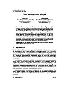
This model seeks the maximum equiproportional reduction in all inputs consistent with observed production. Left-hand side of the input and output constraints represents feasible frontier production assuming constant returns to scale. The Farrell measure is illustrated in input space in Fig. 2.1, where it is assumed that five DMUs (A–E) are observed producing the same output vector Y using two inputs x1 and x2. Data for the DMUs are given in the following chart: DMU A B C D E

X1 5 10 20 30 25

X2 30 20 10 5 25

The input set LC ðYÞ and the associated isoquant Isoq LC ðYÞ are shown. Four DMUs (A–D) are observed producing Y efficiently; it is not possible to reduce both inputs at the same rate while maintaining production of Y. The resulting level of efficiency for these DMUs is 1. DMU E, on the other hand, is observed producing Y using excess inputs; it is possible to reduce both inputs from 25 to 15. We note that an equally weighted convex combination of B and C results in the solution of (2.10). Based on (2.6) and the solution to (2.10), the resulting Farrell efficiency measure would be FC ðYE ; XE Þ ¼ 15=25 ¼ 0:6: Hence, DMU E should be able to produce the same level of output using 60% of its current input levels. We can also illustrate constant returns to scale input-oriented efficiency measurement using the piecewise linear technology (2.9). In Fig. 2.2, we assume for convenience that one input x1 is used to produce one output y1. Data from Fig. 2.2 are given in the following chart:

DMU A B C D E

X1 10 14 20 30 20

Y1 10 20 28.57 32 14

Input-Oriented Models Fig. 2.1 Input-oriented efficiency measurement and Isoq LC(Y)

11 x2 30

A LC (Y) E

25 20

B

15 10

Isoq LC (Y)

C

D 10

Fig. 2.2 Input-oriented efficiency measurement using TC

15

20

25

30

x1

30

x1

y1 D 30

C

B

20

TC

14 10

E A

9.8

20

Variable Returns to Scale DEA While Farrell (1957) introduced the model for efficiency analysis, the model was restrictive with the assumption of constant returns to scale. Farrell and Fieldhouse (1962) extended this model to allow non-decreasing returns to scale. Afriat (1972) provides the variable returns to scale model that was popularized in the operations

12

2 Data Envelopment Analysis

research literature by Banker et al. (1984). Banker et al. (1984) (BCC) show that the addition of a convexity constraint to the CCR model results in a DEA model that allows increasing, constant, and decreasing returns to scale. In addition, BCC provides a decomposition of CCR Farrell efficiency into scale and technical parts. The input set under variable returns to scale is represented by

LV ðYÞ ¼

8 n X > > > lj ykj  yk ; X : > > > > j¼1 > > > > > n X > > > < lj xij  xi ; > > > > > > > > > > > > > > > :

9 > > k ¼ 1; :::; s; > > > > > > > > > > > > = i ¼ 1; :::; m; >

j¼1 n X

lj ¼ 1;

j¼1

lj  0;

j ¼ 1; :::; n:

> > > > > > > > > > > > > > > ;

(2.11)

The associated variable returns to scale, piecewise linear output sets, and technology are represented by

PV ðXÞ ¼

8 n X > > > lj ykj  yk ; Y : > > > > j¼1 > > > > > n X > > > < lj xij  xi ; > > > > > > > > > > > > > > > :

9 > > k ¼ 1; :::; s; > > > > > > > > > > > > = i ¼ 1; :::; m; >

j¼1 n X

lj ¼ 1;

j¼1

lj  0;

j ¼ 1; :::; n

> > > > > > > > > > > > > > > ;

(2.12)

and

TV ¼

8 n X > > > lj ykj  yk ; ðX; YÞ : > > > > j¼1 > > > > > n X > > > < lj xij  xi ; > > > > > > > > > > > > > > > :

9 > > k ¼ 1; :::; s; > > > > > > > > > > > > = i ¼ 1; :::; m; >

j¼1 n X

lj ¼ 1;

j¼1

lj  0;

j ¼ 1; :::; n:

> > > > > > > > > > > > > > > ;

(2.13)

Input-Oriented Models

13

With these representations, the Farrell input-oriented measure of technical efficiency FV ðY0 ; X0 Þ for observed production possibility ðY0 ; X0 Þ is found via the solution to the following linear program: FV ðY0 ; X0 Þ ¼ min y subject to n X

lj ykj  yk0 ;

k ¼ 1; :::; s;

lj xij  y xi0 ;

i ¼ 1; :::; m;

j¼1 n X

(2.14)

j¼1 n X

lj ¼ 1;

j¼1

lj  0;

j ¼ 1; :::; n:

Relative to Fig. 2.1, the variable returns to scale model will produce the same results as the constant returns to scale model. This results because all units are observed producing the same output levels. We illustrate input-oriented efficiency assuming variable returns to scale in Fig. 2.3, which illustrates the technology defined in (2.13). The data in Fig. 2.3 is the same data used in Fig. 2.2, where it was assumed that one output y1 produced from one input x1. y1 D 30

C

B

20 14 10

Fig. 2.3 Input-oriented efficiency using TV

E A TV

10 11.6

20

30

x1

14

2 Data Envelopment Analysis

DMUs (A–D) are technically efficient, producing on the production frontier; it is not possible for any of these DMUs to reduce input levels while simultaneously producing at least as much output. DMU E, on the other hand, is observed producing in the interior of the technology T. DMU E is observed producing 14 units of output while using 20 units of the input. However, a convex combination of DMUs A and B with a weight on A of 0.6 and a weight on B of 0.4 produces the same output using only 11.6 units of the input. As a result, the efficiency of DMU E is FV ðYE ; XE Þ ¼ 11:6=20¼ 0:58:

Output-Oriented Models While the input-oriented measure projects to the boundary of Isoq LðYÞ; the outputoriented measure projects to the boundary of PðXÞ: The output-oriented measure of technical efficiency of DMUj is given by F1 o ðYj ; Xj Þ ¼ maxfy : yYj 2 PðXj Þg:

(2.15)

The Farrell output-oriented measure projects observed production possibilities as far as possible ensuring that the resulting projection is on Isoq PðXÞ: For this book, we consider the output-oriented efficiency measure to be on the range of (0, 1) and hence, invert the distance function. Assuming variable returns to scale, the inverse F~1 V ðY0 ; X0 Þ of the output-oriented measure of efficiency for observed production possibility ðY0 ; X0 Þ is found via the solution to the following linear program: F~1 V ðY0 ; X0 Þ ¼ max c subject to n X

lj ykj  cyk0 ;

k ¼ 1; :::; s;

lj xij  xi0 ;

i ¼ 1; :::; m;

j¼1 n X

(2.16)

j¼1 n X

lj ¼ 1;

j¼1

lj  0;

j ¼ 1; :::; n:

By removing the convexity constraint, we obtain the inverse of the outputoriented measure of technical efficiency under the assumption of constant returns to scale:

Output-Oriented Models

15

F~1 C ðY0 ; X0 Þ ¼ max c subject to n X

lj ykj  cyk0 ;

k ¼ 1; :::; s;

lj xij  xi0 ;

i ¼ 1; :::; m;

(2.17)

j¼1 n X j¼1

lj  0;

j ¼ 1; :::; n:

The output-oriented measures are illustrated in Figs. 2.4 and 2.5. In Fig. 2.4, DMU E is projected assuming constant returns to scale to the frontier, illustrated as the line from the origin through production possibilities B and C. With the assumption of constant returns to scale, any proportional change in inputs leads to the same proportional change in output. Hence, any change in the scale of operation is represented along a ray (plane) from the origin. Assuming constant returns to scale, the benchmark for E is C and the resulting distance measure is F~1 C ðYE ; XE Þ¼ ~C ðYC ; XC Þ¼ 0:49. Hence, leads to an efficiency estimate of F 2857=14. Inverting F~1 C given DMU E’s input level of 20, they produce only 49% (2.14) of the maximum possible output (2.20). The variable returns to scale frontier is illustrated in Fig. 2.5, with increasing returns to scale measured along line segment AB, constant returns to scale along BC and decreasing returns to scale along CD. In the case of the inefficient production possibility E, the projection to the variable returns to scale leads to a benchmark of C. y1 D 30

C

B

20

TC

14 10

Fig. 2.4 Output-oriented efficiency using TC

E A

10

20

30

x1

16 Fig. 2.5 Output-oriented efficiency using TV

2 Data Envelopment Analysis y1 D 30

C

B

20 14 10

E A TV

10

20

30

x1

Since production possibility C is operating along the constant returns to scale portion of the frontier, the resulting efficiency assuming variable returns to scale is F~V ðYC ; XC Þ¼ 0:49: We note that since F~V ðYC ; XC Þ ¼ F~C ðYC ; XC Þ, production possibility C is projected to a constant returns to scale portion of the variable returns to scale frontier.

Measuring Scale Efficiency In this section, we show that solutions to both the variable and constant returns to scale models provide relevant information on returns to scale and scale efficiency. Necessarily, notions of economies of scale exist only along a production frontier. In order to insure that unit is operating on the variable returns to scale frontier, we can apply model (2.14) to project units to the variable returns to scale frontier and remove any technical inefficiency. Then, solving (2.10) allows us to identify other deviations from the constant returns to scale frontier. First, we will consider the input oriented models. The models developed above allow projection to either a constant returns to scale frontier or a variable returns to scale frontier. If the true technology is characterized by variable returns to scale, programming model (2.14) identifies the benchmark for measuring technical efficiency. The constant returns to scale model (2.10) overestimates true technical inefficiency by projecting to a technically infeasible point if the relevant technically efficient benchmark is characterized by either increasing or decreasing returns to scale. If the technically efficient benchmark is operating under constant returns to scale, the solution of (2.10) is feasible as a solution to (2.14) and technical efficiency is not overestimated.

Measuring Scale Efficiency

17

Banker et al. (1984) introduce the concept of most productive scale size consistent with technically efficient production on the constant returns to scale facet of the production frontier. Production that occurs on an increasing or decreasing returns to scale facet is not most productive and hence, scale inefficient.2 The solution of (2.10) provides a composed measure of technical and scale inefficiency. Given that (2.14) provides a measure of technical efficiency relative to the variable returns to scale technology, the ratio of FC ðY0 ; X0 Þ to FV ðY0 ; X0 Þ provides a measure of scale efficiency for production possibility ðY0 ; X0 Þ: SðY0 ; X0 Þ ¼

FC ðY0 ; X0 Þ : FV ðY0 ; X0 Þ

(2.18)

A useful interpretation is that the variable returns to scale measure (the denominator) effectively removes technical inefficiency by projecting the unit to the variable returns to scale frontier; the ratio shows the additional projection that is possible only if increasing or decreasing returns to scale prevails on the frontier. Consider inefficient DMU E in Figs. 2.2 and 2.3. Figure 2.3 illustrates the projection to the technically efficient benchmark on an increasing returns to scale portion of the frontier. Recall that DMU E is observed using 20 units of input x1 instead of the technically efficient input level of 11.6 to produce an output level y1 of 14. Hence, we found FV ðYE ; XE Þ ¼ 0:58: The projection assuming constant returns to scale is shown in Fig 2.2. Assuming constant returns to scale, we found FC ðYE ; XE Þ ¼ 9:8=20¼ 0:49. We note that the technically efficient benchmark (14, 11.6) is on the increasing returns to scale portion of the frontier. The resulting scale efficiency measure for DMU E is SEðYE ; XE Þ ¼ 0:49=0:58 ¼ 0:84. Hence, DMU E is only 84% scale efficient. We note that the scale efficiency of DMU E is equal to 9.8/11.6. The measure of scale efficiency provides a measure of the proximity to most productive scale size (constant returns to scale). This is illustrated in Fig. 2.6. Consider technically efficient DMU A which is the furthest from the constant returns to scale facet BC along the increasing returns to scale facet AB. Starting at DMU A, as x1 increases along the increasing returns to scale facet AB, the inputoriented distance between AB and the constant returns to scale frontier BC decrease. Hence, as a technically efficient benchmark gets closer to the most productive scale size, FV approaches FC and the scale efficiency approaches unity. Alternatively, we can measure scale efficiency using the output-oriented model. ~1 Solving models (2.16) and (2.17), we obtain F~1 V ðY0 ; X0 Þ and FC ðY0 ; X0 Þ, respec1 ~ tively, for production possibility ðY0 ; X0 Þ. In this case, FV ðY0 ; X0 Þ projects the production possibility to the variable returns to scale frontier as the maximum radial expansion in output consistent with observed inputs. The scale efficiency measure for production possibility ðY0 ; X0 Þ using the output oriented model is given by

2

Panzar and Willig (1977) provide a useful discussion of returns to scale in multiple output technologies.

18

2 Data Envelopment Analysis

~1 ~ 0 ; X0 Þ ¼ FV ðY0 ; X0 Þ : SðY F~1 ðY0 ; X0 Þ

(2.19)

C

The interpretation of the scale from the output oriented model is similar to the one from the input oriented model. In Fig. 2.7, we present the output-oriented measure of scale efficiency. In this case, technically efficient DMU A is projected up to the constant returns to scale frontier. As production increases along the y1 D

30 C

20

TC

B

14 10

Fig. 2.6 Input orientation and scale efficiency

A

9.8

20

x1

30

y1 D

30 C

20

TC

B

14 10

Fig. 2.7 Output orientation and scale efficiency

A

9.8

20

30

x1

Measuring Scale Efficiency

19

increasing returns to scale facet AB, the vertical distance between points on AB and the facet from the origin through the B and C narrows. As the technically efficient benchmark approaches most productive scale size B, the scale efficiency of the benchmark approaches 1. Likewise, as production increases along the decreasing returns to scale segment DC away from the most productive scale size C, scale inefficiency decreases as indicated by the larger arrows as the input level increases. The results from the input- and output-oriented models provide information not only about scale efficiency but also about the returns to scale classification. For any ~ 0 ; X0 Þ  1. A benchmark3 is production possibility ðY0 ; X0 Þ, SðY0 ; X0 Þ  1 and SðY operating under constant returns to scale using the P input-oriented model if n  in the SðY0 ; X0 Þ ¼ 1: If the benchmark is scale inefficient, j¼1 lj obtained Pn  solution of (2.10) provides information on the scale class; if l 1; the benchmark is operating under decreasing returns to scale since a most productive scale size production possibility is scaled beyond the constant returns facet. ~ 0 ; X0 Þ ¼ 1, the For the output-oriented models, the same heuristic applies. If SðY associated benchmark is operating under constant returns to scale. If the unit is Pn  scale inefficient, l Þ 1 in the solution of (2.17) identifies increasing j¼1 j (decreasing returns to scale). In this chapter, we introduced standard DEA models that will be used in this book. Models are classified as input or output oriented with either constant or variable returns to scale. These models are the basic DEA models that are widely used in the operations research and economics literatures. Modifications that are needed to apply to analyze baseball will be developed in the relevant chapters as necessary. The goal of this chapter was to present the basic models that serve as the basis for this book. Readers interested in theoretical extensions should consult F€are et al. (1994) and other sources.

3

We refer only to the benchmark to reinforce the notion that returns to scale is not identified for technically inefficient units.

http://www.springer.com/978-1-4419-0830-8