E65: Data Envelopment Analysis

1

E65: Data Envelopment Analysis E65.1 Introduction There are two broad paradigms used by researchers to analyze efficiency in production, stochastic frontier analysis (SFA) and data envelopment analysis (DEA). No formulation has yet been devised that unifies SFA and DEA in a single analytical framework. Arguably, the former is a fully parameterized model whereas the latter is ‘nonparametric,’ albeit also atheoretical in nature. DEA is currently the conventional approach to deterministic frontier estimation. This is usually handled with linear programming techniques. The analysis assumes that there is a frontier technology (in the same spirit as the stochastic frontier production model) that can be described by a piecewise linear hull that envelopes the observed outcomes. Some (efficient) observations will be on the frontier while other (inefficient) individuals will be inside. The technique produces a deterministic frontier that is generated by the observed data, so by construction, some individuals are ‘efficient.’ This is one of the fundamental differences between DEA and SFA. This chapter presents LIMDEP’s programs for data envelopment analysis (DEA).

E65.2 Data Envelopment Analysis Stochastic frontier modeling is based on maximum likelihood or other classical or Bayesian, parametric econometric techniques. In contrast, DEA is based on nonparametric, linear programming methods. Both paradigms are based on an underlying construct of the efficient production frontier that relates maximal output to inputs for the ‘firm’ (decision making unit, or DMU). Using SFA methods, the analyst defines, then estimates a continuous, regular relationship that defines the frontier. DEA uses linear programming methods to fit a piecewise linear ‘hull’ around the data, under the assumption that the hull adequately approximates the underlying frontier, the more so as the number of observations increases. (Since the technique is nonstatistical, this is difficult to establish analytically.) There is a vast literature on the two techniques and comparisons, none of which will be reviewed here. Our purpose here is only to document the estimator. We recommend, as a departure point in the literature, a working paper by Coelli (1996a), which describes the techniques documented here and introduces some of the theoretical notions. He also provides several useful citations.

E65.2.1 Input and Output Oriented Efficiency The discussion of DEA efficiency measurement begins with the notion of a measure of the ratio of outputs to inputs for firm ‘i,’ Ratioi = α′yi / β′xi, i = 1,..,N, where yi is the vector of M outputs and xi is the vector of K inputs. The optimal weights are defined by the programming problem, Maximize wrt α,β: α′yi / β′xi Subject to

α′ys / β′xs < 1, s = 1,...,N αm > 0, m = 1,...,M βk > 0, k = 1,...,K

E65: Data Envelopment Analysis

2

The optimization program seeks the optimal weights to maximize the ‘efficiency’ of firm s subject to the restriction that the efficiencies of all firms are less than or equal to one, and that all weights are nonnegative. Because the objective function is homogeneous of degree zero – any multiple of the weights produces the same solution – it is normalized with a restriction such as α′xi = 1. Transforming and simplifying the problem a bit produces the equivalent program, Maximize wrt α,β: α′yi Subject to

β′xi = 1 α′ys - β′xs < 0, s = 1,...,N α>0 β>0

An equivalent form of the problem is the envelopment form (hence the name), Minimize wrt θi, λ: θi Subject to

Σs λsys – yi > 0 θi xi - Σ λsxs > 0 λs > 0.

The value of θi is the input oriented technical efficiency score for the ith firm TEINPUT,i = θi. It measures the extent to which the firm could reduce inputs to obtain the same output – relative to other firms in the sample. Note that the program is solved for each firm in the sample – an efficiency score θi is generated for each firm. For some firms in the sample, the efficiency score will be 1.0. This indicates firms deemed to be technically efficient. Otherwise, θi < 1. The preceding formulation includes an implicit assumption of constant returns to scale (CRS). The assumption is relaxed to variable returns to scale (VRS), by adding a restriction Σs λs = 1. Variable returns to scale is the standard assumption in contemporary applications. This provides a means by which the ‘scale efficiency’ of the firm can be measured. Let θiC denote the technical efficiency measure obtained assuming constant returns and θiV be the variable returns to scale counterpart. Then, the ‘scale efficiency’ may be measured by SEi = θiC / θiV. This can be computed using the results of the two different programs after computation. A ‘nonincreasing returns to scale’ (NRS) version of the program can be obtained by changing the adding up restriction to Σs λs < 1.

E65: Data Envelopment Analysis

3

An alternative view of the optimization process is to consider the extent to which outputs could conceivably be increased using the same inputs – again relative to the standard of other firms in the sample. The linear program which produces this solution is Maximize wrt φi, λ: φi Subject to

Σs λsys – φi yi > 0 xi - Σ λsxs > 0 λs > 0.

Once again, this assumes constant returns to scale. The variable returns to scale form is obtained by adding the constraint Σsλs = 1. In this solution, 1 < φi < ∞. The technical efficiency measure is 0 < TEOUTPUT,i = 1/φi < 1 As before, some firms in the sample (the same firms) will be found to be technically efficient by this output oriented efficiency measure.

E65.2.2 Economic and Allocative Efficiency With input price information, wi, (and assuming cost minimization) a cost minimization program to find the optimal inputs given the input prices is Minimize wrt χi, λ: wi′ χi Subject to

Σs λsys – yi > 0 χi - Σ λsxs > 0 λs > 0.

As before, to allow for variable returns to scale (VRS), we add Σs λs = 1. In this program, χi gives the cost minimizing vector of inputs for output yi and input prices wi. The cost efficiency for the ith firm is then the ratio 0 < CEi = wiχi / wi′xi < 1. Allocative efficiency may be measured using 0 < AEi = CEi / TEINPUT,i < 1.

E65.2.3 Solutions to the Optimization Problems We note briefly the mathematical form of LIMDEP’s solutions to the linear programs above. The programming problem is defined in terms of • • • • •

Activity vector, γ = the solution vector Coefficient vector, c so that the objective function is c′γ Constraint matrix, A Lower and upper limits for constraints, bL and bU Lower and upper limits for activities, dL and dU

E65: Data Envelopment Analysis

4

The linear program solution, in general is, then, Optimize wrt γ:

c′γ

Subject to

bL < Aγ < bU dL < γ < dU.

We will define the components for the three programs defined earlier. Note, first, for convenience, we define the data matrices, Y and X. Y is an N×M matrix of outputs whose ith row is the vector of outputs for firm i; X is the N×K matrix of inputs, defined likewise. For an individual firm, we define yi to the M×1 column vector of outputs for firm i; thus, yi is the transpose of the ith row of Y. Likewise, xi is the column vector of K inputs for firm i, the transpose of the ith row of X. Finally, the column vector of weights is λ = (λ1,...,λN)′. Thus, Σs λs ys = Y′λ and Σs λs xs = X′λ. Finally, we note once again, the programs about to be defined are solved for each firm to obtain the efficiency scores. (In fact, λ should be indexed by firm, since it is recomputed each time. For convenience, we have omitted this subscript.) We use the symbol ∞K and ∞M to indicate a vector whose each element equals infinity (or sometimes minus infinity) and boldface 1 or 0 to indicate a vector of ones or zeros with a subscript to indicate the number of elements. Finally, our tableaus include the VRS restriction, which may be suppressed by the user for the CRS form. With all this in place, we can define the solutions to the optimization problems just by identifying the components of the linear programming problems. These are as follows:

Input Oriented Technical Efficiency

λ  0  0  1  d L =  N  , c =  N  , γ =   , dU =  N  0 1 1  φi  -∞ K   X′ -xi   0K      b L =  y i  , A =  Y′ 0 M  , bU = ∞ M   1  1′N 0   1  Output Oriented Technical Efficiency

λ  0 N  0 N  d L = , c = ,γ = =  , dU   1 1 φi   −∞ K   X′ 0 K  = b L = 0 M  , A  Y′ = -y i  , bU  1  1′N 0 

1N  ∞    xi  ∞   M  1 

E65: Data Envelopment Analysis

5

Allocative Efficiency

0 N  λ  0 N  , c = ,γ = = d L =   , dU  0 K  wi  χi   −∞ K   X′ -I K   = b L = -y i  , A  Y′ 0= M × K  , bU 0′K   1  1′N

 1N  ∞   Κ  0K    ∞ M   1 

One final note, DEA requires a fair amount of computation. The linear program involves M+K+1 constraints and N+1 activities, and it is computed once for each of the N firms in the sample. The amount of computation increases with the square of N. The particular computations are quite fast, however

E65.3 Confidence Limits for Efficiency Scores A major shortcoming of the DEA approach to modeling production is the absence of a statistical underpinning. One approach that has been used to try to produce some statistical characterization of the estimator is to use bootstrapping to obtain confidence limits for the estimated efficiency scores. A popular method used is that of Simar and Wilson (1984). In brief, their method amounts to the following: We have in hand for each firm a θi estimated using the linear program defined above. To carry out the bootstrap, we use the following experiment. The data on xm for all firms, including this one, are proportionally scaled using a randomly generated (see their paper for the algorithm) scale factor, θi/τmb for replication b. Then, θi,b is recomputed using the revised data, with the same method. The experiment is repeated B times. The 5th and 95th percentiles of the B observations provide the confidence limits. This is repeated B times for each firm. To obtain bootstrapped confidence use the command syntax described below, with the simple addition of the request for the number of bootstrap replications. It should be noted, bootstrapping adds considerably to the amount of computation. In general, the analysis requires the computation of 2N linear programs, two for each firm, to compute the input and output oriented efficiency scores, plus one more if input prices are supplied for the allocative efficiency computation. Bootstrapping adds B×N more programs. Each program involves N+1 activities and K+M+1 constraints, so overall, the amount of computation is considerable. Nonetheless, each component of each linear program is very fast. In the example below, we have 123 observations. We requested 50 bootstrap replications, so we computed altogether 53×123 = 6,519 programs, each with 123 activities. The LP computations plus all the ancillary computations and the display took altogether only 3.84 seconds on our desktop computer.

E65: Data Envelopment Analysis

6

E65.4 Command Structure The command for the data envelopment analysis routine is simply FRONTIER

; Lhs = output variables ; Rhs = input variables (will never include one) ; Alg = DEA $

The following is the full list of specifications for this command. The default specification uses the variable returns to scale form. If you wish to use the constant returns to scale form, add ; CRS to the command. The nonincreasing returns to scale form (Σi λi < 1) is requested with ; NRS If you wish to analyze input price data, add ; Rh2 = input price variables The program computes the DEA efficiency scores (input and output oriented, and economic efficiency), and stores them as variables and as matrices. (See the description in the next section.) If you would like to see a listing of the scores on your screen, in the output window, add ; List to the command. The list of ‘peer’ firms for each observation (see Section E65.5.1 below) may be requested by adding ; Peers to the command. Finally, to obtain bootstrapped confidence limits for the estimator, add ; Nbt = the desired number of replications

E65: Data Envelopment Analysis

7

E65.5 DEA Results This estimator by default computes both the input and output oriented technical efficiency scores. Descriptive statistics for the results are the visible output from the estimator. The following shows an example, using the sample of 1,482 observations on Spanish dairy farms that was examined in Section E33.10.7. This is a one output, four input process. FRONTIER

; Lhs = milk ; Rhs = cows,land,labor,feed ; Alg = DEA $

+---------------------------------------------------------------------------+ | Data Envelopment Analysis | | Output Variables: MILK | | Input Variables: COWS LAND LABOR FEED | | Underlying Technology assumes VARIABLE Returns to Scale. | +---------------------------------------------------------------------------+ | Estimated Efficiencies: Mean Std.Deviation Minimum Maximum | | Technical Efficiency ======= ============= ======= ======= | | Input Oriented .8301 .1416 .4823 1.0000 | | Output Oriented .7388 .1268 .3875 1.0000 | | Sample Size: 1482 Observations. 1482 Complete observations | | Efficiencies saved as variables DEAEFF_O, DEAEFF_I and DEAEFF_E | | Efficiencies saved as matrices DEA_EFFO, DEA_EFFI and DEA_EFFE | | Incomplete observations are filled with zeros for efficiency values. | +---------------------------------------------------------------------------+

As noted, the computed efficiency scores are saved in two places, in the data area, as variables deaeff_i and deaeff_o and deaeff_e if you provide input prices for the economic efficiency analysis. The same results are saved as matrices, dea_effo, dea_effi, dea_effe. Note that in both occurrences, the estimator is bypassing missing and bad (nonpositive) data. If any of the variables used in the analysis are missing, the observation is assigned an efficiency score of 0.0. The matrices will have row dimension equal to the original sample size, before the bypass of missing values. The example below includes a listing of the efficiency scores. The observation identifier shows I = the sequence number of the observation used in the analysis. The R = value shows, instead, the actual location of the observation in the raw data set. I will not equal R if you have used a subset of the data (e.g., with SAMPLE or REJECT), or if the program has bypassed missing data – the listing will only show the complete observations. If you have included observation labels, e.g., firm names, in your data set, these observation and row identifiers will be replaced with the observation names for your data set. For a second example, the following analyzes the Christensen and Greene (1976) electricity generation data. For these data, we have the input prices, so we do the full analysis. FRONTIER

; Alg = DEA ; List ; Nbt = 50 ; Lhs = output ; Rhs = labor,capital,fuel ; Rh2 = lprice,cprice,fprice $

E65: Data Envelopment Analysis

8

+---------------------------------------------------------------------------+ | Data Envelopment Analysis | | Output Variables: OUTPUT | | Input Variables: LABOR CAPITAL FUEL | | Price Variables: LPRICE CPRICE FPRICE | | Underlying Technology assumes VARIABLE Returns to Scale. | +---------------------------------------------------------------------------+ | Estimated Efficiencies: Mean Std.Deviation Minimum Maximum | | Technical Efficiency ======= ============= ======= ======= | | Input Oriented .7692 .1390 .3464 1.0000 | | Output Oriented .7657 .1467 .2960 1.0000 | | Economic Efficiency .4331 .1965 .1411 1.0000 | | Allocative Effic. .5473 .1754 .1796 1.0000 | | Sample Size: 123 Observations. 123 Complete observations | | Efficiencies saved as variables DEAEFF_O, DEAEFF_I and DEAEFF_E | | Efficiencies saved as matrices DEA_EFFO, DEA_EFFI and DEA_EFFE | | Incomplete observations are filled with zeros for efficiency values. | | Compute allocative efficiency as technical divided by economic efficiency | +---------------------------------------------------------------------------+ Estimated Efficiency Values for Individual Decision Making Units (Results are listed only for complete observations) =============================================================================== Observation | Input Oriented| Output Oriented| Economic | Allocative Sample Data | Rank Value| Rank Value| Rank Value| Rank Value ================+===============+================+===============+============= I= 1 R= 1| 1 1.00000| 1 1.00000| 1 1.00000| 1 1.00000 I= 2 R= 2| 13 .98446| 16 .92501| 53 .43644| 87 .44333 I= 3 R= 3| 16 .96243| 28 .88393| 119 .17287| 123 .17962 I= 4 R= 4| 46 .79469| 83 .73593| 96 .29127| 103 .36652 I= 5 R= 5| 115 .57426| 118 .44224| 47 .44703| 15 .77845 I= 6 R= 6| 120 .44307| 122 .35608| 103 .26194| 43 .59120 I= 7 R= 7| 80 .73356| 100 .64826| 101 .26996| 102 .36801 I= 8 R= 8| 123 .34637| 123 .29601| 121 .15388| 85 .44425 I= 9 R= 9| 106 .62517| 110 .57829| 109 .21689| 111 .34692 I= 10 R= 10| 103 .63852| 107 .59578| 66 .38812| 39 .60783 (Remaining observations are omitted.) ---------------------------------------------------------------------------Results of Bootstrap analysis of technical efficiency. 50 replications ---------------------------------------------------------------------------Technical Estimated Corrected Standard Confid. Limits Observation_____ Efficiency Bias Tech.Eff. Deviation Lower Upper I= 1 R= 1 1.0000 .0000 1.0000 .0000 1.0000 1.0000 I= 2 R= 2 .9845 -.0634 1.0479 .1008 .6583 1.0000 I= 3 R= 3 .9624 -.0898 1.0522 .1391 .5023 1.0000 I= 4 R= 4 .7947 .1091 .6856 .0953 .7222 1.0000 I= 5 R= 5 .5743 .3006 .2737 .1215 .6007 1.0000 I= 6 R= 6 .4431 .4318 .0113 .1246 .5785 1.0000 I= 7 R= 7 .7336 .1086 .6250 .1131 .6609 1.0000 I= 8 R= 8 .3464 .5317 -.1853 .0979 .6977 1.0000 I= 9 R= 9 .6252 .2154 .4097 .1265 .5131 1.0000 I= 10 R= 10 .6385 .2267 .4118 .1062 .6645 1.0000

E65: Data Envelopment Analysis

9

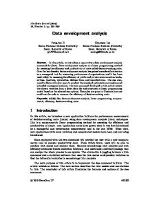
It is always interesting to compare the DEA results with those obtained using the stochastic frontier model. The following fits a translog stochastic frontier production function for the Christensen and Greene data, computes the technical efficiencies, and plots them against the DEA efficiency scores. As has been widely documented, the results are not so close to each other as one might hope. FRONTIER

PLOT

; Lhs = logq ; Rhs = one,logcap,loglabor,logfuel, loglsq,logksq,logfsq,logklogl,logklogf,logllogf ; Techeff = tesf $ ; Lhs = tesf ; Rhs = deaeff_i ; Grid ; Title = DEA Efficiencies vs. Stochastic Frontier JLMS $

Figure E65.1 Comparison of SFA and DEA Efficiency Estimates

E65.5.1 Analysis of Peers Part of the solution for the technical efficiency is the set of activity multipliers, λi,m for the ith firm. The vector of N values, λi,m will give the weights that produce the point on the efficient frontier for this firm. The firms with nonzero values of λi,m – there will typically only be a few or one of them – will define the ‘peers’ for firm i. The listing of the peer firms can be requested by adding ; Peers to the command. The first few observations for the sample above are shown below. =============================================================================== Peers - By Firm =============================================================================== Firm Orient. TechEff Peers --------------------- ------- ------- -------------------------------------1 Inputs 1.00000 3 14 101 Outputs 1.00000 1 14 101 2 Inputs .98446 4 71 Outputs .92501 1 71 3 Inputs .96243 3 71 Outputs .88393 1 71 4 Inputs .79469 4 14 Outputs .73593 1 14 5 Inputs .57426 4 71 118 Outputs .44224 1 71

E65: Data Envelopment Analysis

10

E65.5.2 Application The following uses all the features of the routine save for the Malmquist TFP computation and the allocative efficiency routine. The sample data are in an Excel spreadsheet: IMPORT FRONTIER

; File = … testdea.csv $ ; Lhs = cameras,video,warranty ; Rhs = floor,staff ; Alg = DEA ; CRS ; Peers ; Nbt = 50 $

Figure E65.2 Sample Data for Data Envelopment Analysis +---------------------------------------------------------------------------+ | Data Envelopment Analysis | | Output Variables: CAMERAS VIDEO WARRANTY | | Input Variables: FLOOR STAFF | | Underlying Technology assumes CONSTANT Returns to Scale. | +---------------------------------------------------------------------------+ | Estimated Efficiencies: Mean Std.Deviation Minimum Maximum | | Technical Efficiency ======= ============= ======= ======= | | Input Oriented .9132 .1270 .6387 1.0000 | | Output Oriented .9132 .1270 .6387 1.0000 | | Sample Size: 11 Observations. 11 Complete observations | | Efficiencies saved as variables DEAEFF_O, DEAEFF_I and DEAEFF_E | | Efficiencies saved as matrices DEA_EFFO, DEA_EFFI and DEA_EFFE | | Incomplete observations are filled with zeros for efficiency values. | +---------------------------------------------------------------------------+

E65: Data Envelopment Analysis

11

Estimated Efficiency Values for Individual Decision Making Units =============================================================================== Observation | Input Oriented| Output Oriented| Economic | Allocative Sample Data | Rank Value| Rank Value| Rank Value| Rank Value ================+===============+================+===============+============= Bury | 9 .79126| 9 .79126| 0 .00000| 0 .00000 London | 1 1.00000| 1 1.00000| 0 .00000| 0 .00000 Glasgow | 7 .95227| 7 .95227| 0 .00000| 0 .00000 Bath | 1 1.00000| 1 1.00000| 0 .00000| 0 .00000 Chippenham | 11 .63869| 11 .63869| 0 .00000| 0 .00000 Liverpool | 1 1.00000| 1 1.00000| 0 .00000| 0 .00000 Tunbridge | 8 .90635| 8 .90635| 0 .00000| 0 .00000 Leicester | 1 1.00000| 1 1.00000| 0 .00000| 0 .00000 Malmesbury | 1 1.00000| 1 1.00000| 0 .00000| 0 .00000 Kendal | 10 .75714| 10 .75714| 0 .00000| 0 .00000 Bristol | 1 1.00000| 1 1.00000| 0 .00000| 0 .00000 =============================================================================== Peers - By Firm Firm Orient. TechEff Peers --------------------- ------- ------- -------------------------------------1 Bury Inputs .79126 6 11 Outputs .79126 6 11 2 London Inputs 1.00000 2 Outputs 1.00000 2 3 Glasgow Inputs .95227 2 6 11 Outputs .95227 2 6 11 4 Bath Inputs 1.00000 2 4 8 9 Outputs 1.00000 2 4 5 Chippenham Inputs .63869 6 11 Outputs .63869 6 11 6 Liverpool Inputs 1.00000 6 11 Outputs 1.00000 6 7 Tunbridge Inputs .90635 4 8 9 Outputs .90635 4 8 9 8 Leicester Inputs 1.00000 2 8 9 Outputs 1.00000 2 8 9 Malmesbury Inputs 1.00000 4 6 9 Outputs 1.00000 2 6 9 10 Kendal Inputs .75714 2 4 Outputs .75714 2 4 11 Bristol Inputs 1.00000 2 11 Outputs 1.00000 2 11 =============================================================================== ---------------------------------------------------------------------------Results of Bootstrap analysis of technical efficiency. 50 replications ---------------------------------------------------------------------------Technical Estimated Corrected Standard Confid. Limits Observation_____ Efficiency Bias Tech.Eff. Deviation Lower Upper Bury .7913 .0404 .7509 .0374 .7931 .9074 London 1.0000 .0000 1.0000 .0000 1.0000 1.0000 Glasgow .9523 .0353 .9170 .0143 .9570 1.0000 Bath 1.0000 .0000 1.0000 .0000 1.0000 1.0000 Chippenham .6387 .0392 .5995 .0309 .6411 .7293 Liverpool 1.0000 .0000 1.0000 .0000 1.0000 1.0000 Tunbridge .9064 .0630 .8433 .0333 .9138 1.0000 Leicester 1.0000 .0000 1.0000 .0000 1.0000 1.0000 Malmesbury 1.0000 .0000 1.0000 .0000 1.0000 1.0000 Kendal .7571 .0389 .7183 .0551 .7614 .9307 Bristol 1.0000 .0000 1.0000 .0000 1.0000 1.0000 ----------------------------------------------------------------------------

E65: Data Envelopment Analysis

12

E65.6 Comparing Efficiency Values and Rankings – SFA vs. DEA In many settings, the efficiency ratings themselves are less interesting than the ranks of the observations. The WHO study used in numerous examples throughout this chapter is an example, in which the objective of the efficiency analysis was to rank the countries in terms of their measured efficiency. A perennial question in the efficiency analysis literature focuses on whether one obtains the same qualitative results with the two methodologies. We return to the WHO data to provide an illustration. The data used are the country means of the output, dale, and two inputs, health expenditure, hexp, and education, educ. After the raw data are input, we use the following SAMPLE REJECT CREATE CREATE CREATE REJECT CREATE CREATE CREATE FRONTIER FRONTIER DSTAT PLOT PLOT CREATE CREATE CREATE CALC

PLOT

PLOT

; All $ ; Small > 0 $ ; dalebar = Group Mean(dale, Str = country) $ ; hexpbar = Group Mean(hexp, Str = country) $ ; educbar = Group Mean(educ, Str = country) $ ; year # 1997 $ ; logdbar = Log(dalebar) $ ; loghbar = Log(hexpbar) $ ; logebar = Log(educbar) $ ; Lhs = logdbar ; Rhs = one,loghbar,logebar ; Techeff = effsfa $ ; Lhs = dalebar ; Rhs = hexpbar,educbar ; Alg = DEA$ ; Rhs = effsfa,deaeff_i,deaeff_o ; Output = 2 $ ; Lhs = effsfa ; Rhs = deaeff_i ; Grid ; Title = SFA Efficiencies vs. DEA Input Efficiencies $ ; Lhs = effsfa ; Rhs = deaeff_o ; Limits=.4,1.1 ; Grid ; Title = SFA Efficiencies vs. DEA Output Efficiencies $ ; sfarank = Rnk(effsfa) $ ; dearanki = Rnk(deaeff_i) $ ; dearanko = Rnk(deaeff_o) $ ; List ; Rkc(sfarank,dearanki) ; Rkc(sfarank,dearanko) ; Rkc(dearanki,dearanko) $ ; Lhs = sfarank ; Rhs = dearanki ; Endpoints = 0,200 ; Limits = 0,200 ; Grid ; Title = Ranks of SFA Efficiencies vs. DEA Input Efficiencies $ ; Lhs = sfarank ; Rhs = dearanko ; Endpoints = 0,200 ; Limits = 0,200 ; Grid ; Title = Ranks of SFA Efficiencies vs. DEA Output Efficiencies $

E65: Data Envelopment Analysis

13

Normal exit: 11 iterations. Status=0, F= -133.3834 ----------------------------------------------------------------------------Limited Dependent Variable Model - FRONTIER Dependent variable LOGDBAR Log likelihood function 133.38343 Estimation based on N = 191, K = 5 Inf.Cr.AIC = -256.8 AIC/N = -1.344 Variances: Sigma-squared(v)= .00140 Sigma-squared(u)= .04405 Sigma(v) = .03744 Sigma(u) = .20989 Sigma = Sqr[(s^2(u)+s^2(v)]= .21320 Gamma = sigma(u)^2/sigma^2 = .96915 Var[u]/{Var[u]+Var[v]} = .91947 Stochastic Production Frontier, e = v-u LR test for inefficiency vs. OLS v only Deg. freedom for sigma-squared(u): 1 Deg. freedom for heteroscedasticity: 0 Deg. freedom for truncation mean: 0 Deg. freedom for inefficiency model: 1 LogL when sigma(u)=0 114.81039 Chi-sq=2*[LogL(SF)-LogL(LS)] = 37.146 Kodde-Palm C*: 95%: 2.706, 99%: 5.412 --------+-------------------------------------------------------------------| Standard Prob. 95% Confidence LOGDBAR| Coefficient Error z |z|>Z* Interval --------+-------------------------------------------------------------------|Deterministic Component of Stochastic Frontier Model Constant| 3.57889*** .04980 71.87 .0000 3.48129 3.67649 LOGHBAR| .06480*** .00824 7.86 .0000 .04864 .08096 LOGEBAR| .15292*** .01852 8.26 .0000 .11662 .18923 |Variance parameters for compound error Lambda| 5.60534*** 1.46657 3.82 .0001 2.73091 8.47977 Sigma| .21320*** .00101 211.97 .0000 .21123 .21517 --------+-------------------------------------------------------------------Note: ***, **, * ==> Significance at 1%, 5%, 10% level. ----------------------------------------------------------------------------+---------------------------------------------------------------------------+ | Data Envelopment Analysis | | Output Variables: DALEBAR | | Input Variables: HEXPBAR EDUCBAR | | Underlying Technology assumes VARIABLE Returns to Scale. | +---------------------------------------------------------------------------+ | Estimated Efficiencies: Mean Std.Deviation Minimum Maximum | | Technical Efficiency ======= ============= ======= ======= | | Input Oriented .6138 .2089 .2059 1.0000 | | Output Oriented .8794 .1124 .5061 1.0000 | | Sample Size: 191 Observations. 191 Complete observations | | Efficiencies saved as variables DEAEFF_O, DEAEFF_I and DEAEFF_E | | Efficiencies saved as matrices DEA_EFFO, DEA_EFFI and DEA_EFFE | | Incomplete observations are filled with zeros for efficiency values. | +---------------------------------------------------------------------------+ --> DSTAT ; Rhs = effsfa,deaeff_i,deaeff_o ; Output = 2 $

E65: Data Envelopment Analysis

14

Descriptive Statistics --------+--------------------------------------------------------------------Variable| Mean Std.Dev. Minimum Maximum Cases Missing --------+--------------------------------------------------------------------EFFSFA| .882053 .059219 .801579 .982272 191 0 DEAEFF_I| .613836 .208905 .205870 1.0 191 0 DEAEFF_O| .879363 .112447 .506133 1.0 191 0 --------+----------------------------------------------------------------------------+-------------------------Cor.Mat.| EFFSFA DEAEFF_I DEAEFF_O --------+-------------------------EFFSFA| 1.00000 .70610 .75911 DEAEFF_I| .70610 1.00000 .72559 DEAEFF_O| .75911 .72559 1.00000

Figure E65.3 Plot of SFA Efficiency Values vs. DEA Values

E65: Data Envelopment Analysis

Figure E65.4 Plot of Ranks of SFA Efficiency Scores vs. Ranks of DEA Scores

15

E65: Data Envelopment Analysis

16

E65.7 Malmquist Index of Total Factor Productivity (Once again, the user is referred to the relevant literature, such as the numerous papers by Fare and Grosskopf) for background details. Fare’s 1994 output based Malmquist productivity change may be written M i,O (t,t + 1) =

TEi (t + 1 | t ) × TEi (t + 1 | t + 1) TEi (t | t ) × TEi (t | t + 1)

where TE(r|s) indicates the earlier defined output oriented technical efficiency index for firm i, using inputs xi,r and producing outputs yi,r relative to production (and input usage) for firms based in period s. This index is computed using the following program:

λ 0 N  0 N  1  , c = ,γ  = , dU  N  = d L =    0 1 ∞ φir   X′ 0 K   −∞ K  x  ,A  s = , bU  i  = b L =    0M  ∞ M   Ys′ -y ir  This uses the constant returns to scale form. Also, since the period r output and input vectors for firm i will not appear in Ys and Xs when r does not equal s, φir need not be larger than one. Note that this requires solution of four linear programs for each firm in each period, so the total number of programs to solve will be 4×N×T. Each is quite fast, so overall, the computations do not take long. In the sample of 247 firms and six periods, the nearly 6,000 programs, each involving 248 activities and six constraints, took about 10 seconds. These computations are carried out for each firm in each period save the last one, and produce an N×T matrix of TFP values, one row for each firm, one column for each period. The TFP value for the last period is recorded as 1.0, though this is just a space filler. To compute the Malmquist TFP indices, you will require a panel of data, at least two periods, for each of N firms. Unlike other panel data routines in LIMDEP, this computation always requires a balanced panel. Every firm must be observed in the same T periods. Also, this routine has no procedures for avoiding missing or invalid data such as zero values for inputs or outputs. The balanced panel must be ‘clean’ before computation begins. To request the computations, just add ; Pds = t, the fixed number of periods. Nothing else need be changed. There is no bootstrap feature (; Nbt = 0); the computations assume constant returns to scale (; CRS is the default and cannot be changed) and no allocative efficiency (; Rh2 is ignored).

E65: Data Envelopment Analysis

17

Malmquist TFP Index Application To illustrate the Malmquist computations, we reexamine the sample of 247 Spanish dairy farms observed for six years. The output is milk production. Inputs are cows, land, labor and feed. FRONTIER

; Lhs = milk ; Rhs = cows,land,labor,feed ; Alg = DEA ; Pds = 6 ; List $

The following results are displayed. malmquist, is created.

In addition, a matrix containing the full table, named

============================================================================== Malmquist TFP Index for Productivity Change Panel contained 247 firms each observed in 6 periods Full Results saved as matrix MALMQIST ============================================================================== Average results across firms, by period: ============================================================================== Period: 1 2 3 4 5 TFP 1.0476 1.0233 1.0247 1.0298 1.0349 ============================================================================== Individual calculations by firm (Only 8 periods can be displayed. TFP for the final period is not computed.) ============================================================================== Observation 1 2 3 4 5 6 7 8 Firm = 1 1.1301 1.1002 .9736 1.0291 1.0901 1. Firm = 2 1.0528 1.0343 1.0212 1.0109 1.0416 1. Firm = 3 1.0525 1.0383 .9477 1.0465 1.0395 1. Firm = 4 1.1418 1.0129 1.0079 .9829 1.0476 1. Firm = 5 1.1192 1.0240 1.0082 1.0245 1.0641 1. Firm = 6 .9871 1.0073 .9785 1.0322 1.0464 1. Firm = 7 .9851 1.1484 1.1599 .8054 1.1110 1. Firm = 8 1.0746 .9796 .9636 1.0671 .9753 1. Firm = 9 .8977 1.1496 .9818 1.0500 .9867 1. Firm = 10 1.0105 1.1507 .9751 1.0055 1.0469 1. Firm = 11 1.1276 .9867 .9636 1.0826 .9873 1. Firm = 12 1.0310 1.1020 .9822 1.0438 .9914 1. Firm = 13 1.0549 1.1263 .9221 1.0723 1.1945 1. Firm = 14 .9408 1.0740 .9938 .9739 1.0336 1. Firm = 15 .8952 .7156 1.5056 .8614 .9204 1. (Rows 66 – 247 omitted).