The European Journal of Comparative Economics Vol. 9, n. 3, pp. 425-443 ISSN 1824-2979

Efficiency in human Development: a Data Envelopment Analysis Valérie Vierstraete1 GREDI- Sherbrooke University Abstract: The human development index (HDI) is a measure of development which allows countries’ development to be assessed on the basis of three indicators that measure the health, education, and standard of living of the population. The UNDP also computes a human development index that excludes this last indicator, the non-income HDI. The HDI, like the non-income HDI, presents some striking intercountry disparities. In this study, we wish to demonstrate that inefficiency in the utilization of financial resources can have an incidence on non-income HDI scores. Thus, owing to a certain “waste” in their use of resources, countries with similar levels of spending may end up with differing levels of human development. We measure this efficiency using the Data Envelopment Analysis (DEA) method.

JEL Classification : O15, O57, D24, H5 Keywords: Data Envelopment Analysis, efficiency, development, human development index, non-income HDI

1. Introduction In 1990, the first Human Development Report, published by the UNDP (United Nations Development Programme), introduced a new development indicator developed by a task force working under the guidance of Mahbub ul Haq. For many years, the only available measure of development had been per capita GDP, so the UNDP proposed the human development index (HDI) to rank the nations of the world with respect to the state of their human, not only economic, development. The UNDP has published this indicator, along with the associated country rankings, every year since 1990. While it has been subject to some criticism, its computational simplicity has given it a wide following. However, since the 2010 Human Development report, the UNDP has adopted a new methodology for measuring the HDI as well as new indicators of development (for example, the Multidimensional Poverty Index, MPI). Nonetheless, we may ask why some countries that seem similar, especially in terms of their economies, and that have comparable GDP or per capita GDP results, post divergent HDIs. For example, while Chile and Gabon are, respectively, 50th and 49th globally in terms of per capita GDP, in 2009, Chile was ranked 44th overall with respect to the HDI while Gabon languished in 108th position. This may suggest that some countries devote little or no expenditures specifically to human development. Conversely, they may be investing resources in education and healthcare, but in a fashion that is inefficient or wasteful and thus not yielding the desired results: a more educated and healthier population. This is what we want to verify in this article. Using classical and bootstrapped Data Envelopment Analysis (DEA) models, we will seek to determine whether past or current expenditure levels in these countries are yielding an optimal HDI—i.e. the “best” possible HDI in light of the resources invested. In an economic downturn, it seems reasonable to verify the efficiency of countries in achieving their objectives. In this paper, it is the objective of human development that we analyze. 1

[email protected]

Available online at http://eaces.liuc.it

426

EJCE, vol.9, n.3 (2012)

The remainder of this paper is structured as follows. In the second part we review the definition of the human development index and briefly examine the literature. In Part 3, we present the DEA method and, in Part 4, the data. Part 5 contains our results and is followed by the conclusion.

2. The Human Development Index According to the UNDP, personal incomes represent one indicator of a country’s level of human development. However, it is not the only one. Thus, a country with high incomes, as might be generated by resource extraction, for example, will not have a very strong growth potential if these revenues are primarily devoted to expenditures on consumption and imports2. Conversely, this potential may exist if there is investment in individuals. This might, for instance, take the shape of investing in citizens’ education or health. For this reason, the HDI is a composite indicator consisting of two elements in addition to gross national income (GNI). Human health is measured by individuals’ ability to live long lives in good health. The first element in the HDI is thus life expectancy at birth. The second component of the HDI captures populations’ knowledge. This indicator is decomposed into a measure of mean- and expected- years of schooling. Finally, the log of per capita GNI is the third component of the HDI, measuring the ability to access resources, in particular healthcare and education. Thus, the HDI is measured as the geometric mean of these three indicators: health, education, and income. The value of the HDI falls between zero (0) and one (1), where one indicates the maximal value of human development and zero a deplorable lack thereof. In 2011, the HDI ranged from 0.286 (Democratic Republic of the Congo) to 0.943 (Norway). The UNDP also computes a non-income HDI that only accounts for the health and education indicators. By publishing this indicator in its 2010 report, the UNDP wanted to reaffirm that development is more than GNP and establish the important role of education and health in development. In 2011, the non-income HDI ranged from 0.311 (Niger) to 0.979 (Australia). Since its inception, numerous studies have examined the HDI. Some of these addressed the methodological rationale for this indicator, suggesting that other factors should be included in the index (Sagar and Najam, 1998; Dar, 2004), or criticizing the arbitrary weighting of the three elements in the indicator, or their aggregation (Chowdhury and Squire, 2006; Noorbakhsh, 1998; Chatterjee, 2005; Cherchye et al., 2008). They argue that changes to how the HDI is calculated would result in a reranking of countries3. Moreover, Srinivasan (1994) and Cahill (2005) suggest that the HDI might be redundant, as income is correlated with education and healthcare. In light of these criticisms, other authors have questioned whether alternative weights could be applied or whether there might be better indicators of countries’ performances. Thus, Mahlberg and Obersteiner (2001), Despostis (2005a, 2005b), Lee et al. (2006), and Lozano and Gutiérrez (2008) use a DEA methodology to compute the appropriate weight for each component of the HDI. In addition, the HDI could be viewed as an inappropriate indicator of countries’ performance. Malul et al. (2009) measure this performance by per capita GDP and the inverse of the Gini index; Nardo et al. (2005) suggest using a composite index with components identified by principal components analysis or cluster analysis and weighted by DEA; Rotberg (2004) emphasizes the 2 3

Unless these are imports of capital goods. The “new” HDI shows thus some changes in the country ranking.

Available online at http://eaces.liuc.it

Valérie Vierstraete, Efficiency in human Development: a Data Envelopment Analysis

427

importance of ranking countries by the quality of their governance, which can be assessed using different proxy indicators or sub-indicators; and Afonso et al. (2010) and Afonso and St Aubyn (2011) evaluate the efficiency with which public expenditures contribute to attaining the individual objectives of education, health, or social protection. As for Arcelus et al. (2005), they measure countries' performance in reaching a high HDI as a function of the resources they devote to it. We base our research on this last study. Using DEA, we verify the countries’ efficiency of reaching a high level of human development, compare this efficiency by regions and use a bootstrapped method to confirm these efficiency results. After reviewing the DEA method in the next section, we will describe the variables we retained for this study.

3. The DEA Method In order to assess countries’ efficiency in achieving a certain value of the HDI, we will perform inter-country comparisons and hold their results up to a target. The DEA method allows us to determine this target, which is defined by the best performers in the sample. Since we are measuring the efficiency of various countries against each other, this is a relative measure. If other countries were included in the study, the efficiency of some of those present would change. An alternative approach to measuring efficiency would be a parametric method, stochastic frontier analysis (SFA) developed by Aigner et al. (1977) and Meeusen and van den Broeck (1977). DEA and SFA present their own advantages and drawbacks. As an econometric method, SFA allows for some noise while DEA assumes all deviations from the frontier are basically due to inefficiency. However, DEA doesn’t require any assumptions other than free disposal and convexity4 and accommodates several inputs and outputs. Furthermore, no explicit functional form is needed for the production frontier with DEA. Another disadvantage of DEA is that the results of efficiency are sensitive to changes to the sample. The frontier can only be composed by the units in the sample. These units could thus be efficient relative to the others in the sample but inefficient compared to units outside the sample. Bootstrap techniques have been developed to solve this sampling problem. As we appreciate the flexibility that allows the DEA method, we chose to measure the countries’ efficiency by this method. Technical efficiency ascertains whether a country is operating on its production frontier. The Banker, Charnes and Cooper (1984) (BCC) DEA model uses linear programming methodology to compute technical efficiency. The goal is to maximize the quantity of output a country is able to generate so as to arrive at the production frontier. In this study, we suppose countries use several inputs in order to maximise their development level. Although we could propose different objective functions, we assume countries promote human development to go with economic development. Our assumption is that economic development is mainly supported by human capital in the long run (Lucas, 1988; Romer, 1990). We thus assume countries maximise their Human Development Index. An input-oriented approach could have been used. Nonetheless, we retain an output-oriented approach because it appeared plausible to us that countries would prefer maximizing the HDI for a given level of resource investment over minimizing the inputs, or resources, for a given level of HDI.

4

The Free Disposal Hull analysis (FDH) can measure efficiency without this convexity assumption.

Available online at http://eaces.liuc.it

EJCE, vol.9, n.3 (2012)

428

Thus, we consider N countriesn (n = 1 ... N). Each country uses R variable inputs xr,n (r = 1 ... R) to produce M outputs ym,n (m = 1 ... M). National technologies are approximated by Farrell’s method (1957). The model is resolved n times (each country is designated unit 0, the reference unit, in turn) using the following linear program: M ⎛ R ⎞ Max φ − ε ⎜ ∑ s r− + ∑ s m+ ⎟ φ ,λ m =1 ⎝ r =1 ⎠

such that: N

∑λ

n

y m ,n − sm+ = φy m ,0

n

x r , n + s r− = x r , 0

n =1 N

∑λ n =1 N

∑λ n =1

n

m = 1K M r = 1K R

(1) (2)

=1

(3)

λn ≥ 0 n = 1... N

Constraints (1) and (2), in conjunction with the assumption of free disposal, allow the theoretical production frontier to be delineated. In constraint (1), the output of country0 is multiplied by the coefficient φ, which allows the production frontier to be reached given the input set x. Constraint (3) renders the free-disposal set locally convex using the vector of weights λn. This constraint yields a variable returns to scale (VRS) technology. Without this constraint, the frontier would reflect a constant returns to scale (CRS) technology. sm+ and sr- are slack variables and ε is a non-Archimedian element allowing the objective function to be solved in two steps (maximization of φ being the first step). Technical efficiency is measured by φ. An efficient unit is characterized by φ = 1 and an inefficient unit by φ > 1. The greater φ, the more inefficient the country is deemed to be. In figure 1, the VRS frontier is composed by the efficient countries, A, B, C, and D. Country E’s technical efficiency is measured by φVRS in the output orientation with a variable returns to scale (VRS) technology.

Available online at http://eaces.liuc.it

Valérie Vierstraete, Efficiency in human Development: a Data Envelopment Analysis

429

Figure 1: Technical Efficiency Φ in an output orientation depending on the returns to scale

In order to solve the sampling problem we refer to, we’ll use one bootstrapped DEA model in this paper following Simar and Wilson (1998). Furthermore, since we only observe the expenditures and outcomes for a subset of countries, the simple DEA method tends to overstate efficiency scores and a bias is created. The bootstrapped DEA (Simar and Wilson, 2004) allows us to correct for the bias in the efficiency scores and to determine the confidence intervals within which the corrected efficiency is most likely to fall.

4. Variables and data To conduct our research we drew on World Bank data available in the World Development Indicators Online (WDI) database. This database provides access to many indicators of development, for more than 200 countries, starting with 1960. However, many data points, for both indicators and years, are missing. Because of the missing data we selected an initial sample of 146 countries with a median per capita GDP of $8 000 (all monetary data has been converted into constant 2005 U.S. dollars using the purchasing power parity method). The HDI data are available from UNDP. Since the HDI is the average of the education, health, and per capita GNI indicators, it appeared problematic to us to treat it as a function of expenditures, which are themselves computed from GNI. For this reason, we opted to explain non-income HDI, which is the geometric mean of health and education indicators. Thus, we will be assessing the efficiency with which the highest possible non-income HDI (our output) is reached as a function of assorted variables that serve as inputs. Obviously we cannot be certain that countries have maximizing the non-income HDI as their objective function. However, since every country in our sample spends on education and healthcare, we can readily assume that these countries have the objective, directly or indirectly, of maximising the items included in the calculation of the non-income HDI. However, it is probable that some countries prioritize education and healthcare differently from the weights implied by the HDI allocation. For this reason, we next assess countries'

Available online at http://eaces.liuc.it

430

EJCE, vol.9, n.3 (2012)

efficiency on the assumption that they weight education and healthcare indicators differently. In order to explain the level of education (level of health, respectively) attained in the countries considered, our approach is to consider expenditures on education (or healthcare, respectively). However, these data are missing when long periods of time are considered. To mitigate this problem, we use a stock variable (stock in the year 2005 as an explanatory variable for the non-income HDI in the year 2011). This stock is assumed to represent all expenditures having been made prior to the date considered. Thus, for health and longevity, we use the number of nurses and midwives per 1000 people. In our opinion, the number of nurses and midwives present in the year 2005 should reflect healthcare related expenditures in preceding years. Our first factor of production is thus the number of nurses and midwives per 1000 residents. The average annual flow of healthcare spending from 2006 to 2010, for a non-income HDI in 2011, is the second production factor considered. These expenditures are expressed per capita. A stock and a flow also represent the nation's education-related factors of production. Thus, per capita expenditure on education is the third input retained. These outlays are considered to represent the country’s commitment to fostering its citizens’ education and training. However, since spending during any one earlier year cannot have a direct impact on literacy in a given year, we considered all previous expenditures. Since some of this data is missing,5 we take as our final production factor a stock that summarizes all past spending. The stock retained is the number of secondary education teachers, per 1000 citizens. The inclusion of certain inputs can be open to debate. For example, as our sample includes developed and developing countries, the choice of inputs representing the stock of past expenditures may be questioned. Indeed, we may wonder whether these inputs better represent a stock of expenditure in a developed country rather than in a developing country. However, as we prefer to ensure the homogeneity in our data, we kept the data from WDI database as far as possible. This limits the availability of stock variables. We tried several stock variables for both education and healthcare, to assess whether this might affect the level of efficiency obtained. Thus, for example, in addition to the model in which we use the number of nurses to represent the healthcare “stock” variable, we also considered measuring the stock of healthcare with the number of physicians per 1000 citizens or the number of hospital beds per 1000 citizens. These two latter inputs have the merit of allowing us to have a larger sample, but they may sometimes be detrimental to LDCs. This is why, inasmuch as possible, we opt for the model with the input “nurses” from here on. We proceed similarly for the input representing the stock of education. We selected the input “number of secondary teachers per 1000 citizens”, but since that limits the number of countries we can include in our model, we reran the analysis with alternative inputs representing the labour force having a secondary (or tertiary) education per 1000 residents. Also, we initially wished to take into account total expenditures on health and education. Indeed, for some countries, it is undeniable that private expenditure on health and education represents an important part of total expenditure. However, while the WDI database gives the total (public and private) expenditures on healthcare, only the public component of education expenditures are provided. For private spending on education, we referred to the UNESCO Institute for Statistics. However, the number of 5

The retained education-related spending is thus mean per capita expenditures between 2006 and 2010.

Available online at http://eaces.liuc.it

Valérie Vierstraete, Efficiency in human Development: a Data Envelopment Analysis

431

countries for which data are available then decreases dramatically. We have to respect the constraint described by Cooper et al. (2004) with regard to the number of different inputs and outputs relative to the number of countries. Decreasing the number of countries would result in a greater proportion of them being considered efficient, simply as an artefact of the absence of similar countries to serve as a reference. Therefore, this model including private spending on education will only be used for comparison purposes. Moreover, we wanted to take into account the fact that countries in our sample are at different economic and social levels. Consequently, comparing all the countries with each other could be seen as a disadvantage for the least developed countries. That is why, by using the Banker and Morey (1986) approach, we grouped countries according whether they are considered developed (favourable situation) or not (unfavourable situation) according to the UN. Thus, we introduce an additional input, a dichotomous variable, to control for this factor. Countries evolving in the most unfavorable environment will be compared among themselves only, in order to not be considered inefficient because of the competition they would face from developed countries. Countries evolving in the environment considered the most favorable will then be compared with all countries. This will correspond to another model the results of which we will interpret. Finally, for all the models we proposed, we used the “windows analysis” technique, which treats each observation on a country as a different unit. This allows, on the one hand, the number of total units we consider to be increased, and on the other hand, the efficiency of each country to be tracked (Charnes et al. 1985). We have collected data for three periods, corresponding to a HDI in 2011, in 2005, and in 2000. Unfortunately all data weren’t available for all variables in all periods. Some of the models will thus not allow intertemporal comparisons. Different DEA models have been run. Table 1 in the appendix summarizes these models. Descriptive statistics for the benchmark model data (Table 2) and the list of countries retained can also be found in the appendix.

5. Results 5.1 Technical efficiency The results of the output-oriented DEA with variable returns to scale when (total) private and public expenditures in education and healthcare are considered are summarized in table 3 (models 1, 2 and 3). Unsurprisingly, more countries are considered efficient in model 1 — meaning that they obtain an efficiency score of φ = 1 — than in the others. As already mentioned, we must bear in mind that this high percentage of countries considered efficient may be an artefact of our sample size. Indeed, in the absence of comparisons, a country may be deemed efficient on the basis of local dominance. Nevertheless, the results across the three models are relatively close, with an average efficiency coefficient φ of 1.04 to 1.06. This indicates that, if the average non-income HDI of the examined countries is 0.7996, they could attain an average nonincome HDI of 0.84 if they were to successfully emulate the best performers. Thus, we

6

Model 2, with 114 units (countries in three periods)

Available online at http://eaces.liuc.it

432

EJCE, vol.9, n.3 (2012)

can say that, on average, there is little resource waste. Past and current expenditures destined to improve the level of human development seem to reach their objectives7. In order to increase the number of countries under study, we replaced the input “total spending on education” by “public spending in education”. We know that some countries rely heavily on private spending in education, but we assume in models 4 to 10, that that affects higher education more than primary or secondary education. In these models, mean inefficiency is slightly higher than in the first ones, except for model 4 where mean inefficiency reached 1.10 (cf. table 3). This is mainly due to developing countries now included in the database, for which information was unavailable in models 1 to 3 and whose inefficiency is higher. Except for this point, it thus seems that the choice of the inputs affects only little the average levels of inefficiency. As we do not want to appear to disadvantage developing countries when compared to developed countries, in models 11 and 12 we included a dummy variable taking into account countries’ economic environment. As we might expect, average efficiency does not differ too much after taking into account this environment. For example, average efficiency decreases from 1.101 to 1.097 between model 4 and model 11. This means that developing countries do not seem disadvantaged by the comparison with developed countries when we measure their efficiency in achieving their nonincome HDI. Even if this may not seem intuitive, this makes senses when we remember that the DEA in a VRS approach allows a comparison of countries which are close to each other in terms of inputs and output. In fact, the only countries which seem to benefit from the inclusion of a dichotomous variable are transition countries (Hungary, Poland, Croatia from the former Eastern bloc, or Qatar, for example, in 2011), which see their level of inefficiency decrease when they are treated as developing countries. However, we observe that a Spearman rank correlation test reveals a weak but significant positive correlation between the ranking of countries by their non-income HDI and by their efficiency. This means that countries reporting a high level of nonincome HDI are also more efficient in their resource utilization. This might be very encouraging for countries that currently have a low HDI, for whom a rationalization of expenditures could result in better performance at the level of human development without necessarily requiring the commitment of supplementary resources.

5.2 Efficiency by region and intertemporal comparisons If we refer to model 11, we note that all countries posting above-average inefficiency are developing countries in 2011 (cf. table 4 which presents the ratio of computed efficiency to mean efficiency for each country in 2011). In that way, countries with the worst inefficiency are mostly Sub-Saharan countries. For example, the inefficiency score for Mali is 1.698, indicating that this country could increase its nonincome HDI by 69% with the same inputs. Nevertheless, even among Sub-Saharan countries strong divergences appear. For example, Togo needs “only” to increase its output by 17% to be considered efficient. Disparities among these countries are explained in a companion paper (Miningou and Vierstraete, 2010)9. Referring to Table 5 We recalculate the non-income HDI if the countries were efficient and compare the actual rank and the rank if each country was efficient. Results are available on request. 8 Table 4 shows an efficiency ratio of 1.516 for Mali. 9 We observe that, accounting for countries only in 2011 (i.e. omitting 2000 and 2005) to conduct the DEA analysis leaves the results virtually unchanged. Indeed, inefficiency levels are practically unchanged. Results are available on demand. 7

Available online at http://eaces.liuc.it

Valérie Vierstraete, Efficiency in human Development: a Data Envelopment Analysis

433

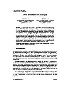
which presents efficiency levels by region in 2011, we easily detect that the region of origin partially explains the levels of efficiency attained by the countries. Thus, with an inefficiency score of 1.2, sub-Saharan Africa posts the highest inefficiency level and it is, along with the Arab countries, one of two regions with a level of inefficiency that exceeds the global average. While developed countries have the lowest inefficiency level in our sample, we observe that the mean inefficiency of the countries of Eastern Europe and Latin America is very close to this minimum10. This appears to show that, in light of past and current expenditures in healthcare and education, countries in transition have the same health and education outcomes as developed countries. Model 11 does not allow us to conduct a comparison to assess the evolution of efficiency over time, because there is a lot of missing data in this specification for the year 2000. We use Model 7 to test whether countries show an improvement in their efficiency between 2000 and 2011. However, we find that certain regions of the world are very poorly represented, so that some results reflect the mean for only two or three countries and need to be used with caution (cf tableau 6). Thus, while we concluded earlier that the countries of Africa posted high inefficiency scores, we now find that the inefficiency levels of countries represented by this specification declines over time, finishing at levels that are comparable to those of developed countries11. Figure 2 reveals that it is principally countries with initially high levels of inefficiency that have posted an improvement over this period. In all likelihood, this reflects a rationalization of expenditures, which became necessary following the economic downturn of 2001 and the crisis of 2008/09. In the case of less inefficient countries, this belt-tightening appears to have been more difficult, in particular in the countries of East Europe, where inefficiency score rose slightly over this period. We observe, in addition, that this is the only zone that experienced such an increase. Tandberg and Pavesic-Skerlep (2009) indicate that, over the past decade or so, many countries in South East Europe have reduced their defense and government administration budgets to reallocate more to healthcare, education, and social services, though results in terms of educational and health outcomes have been slow to materialize. In fact, after the collapse of the communist empire, despite the fact that the countries of Eastern Europe largely benefited from a relatively large human capital stock, this rapidly deteriorated in the wake of the budgetary reorganization these countries experienced (Simai, 2006). An increase in expenditures, in conjunction with a decline in education and health outcomes, thus explains the decreased efficiency in this zone.

Recall that, in this specification, developed countries are compared with all countries in the sample, while the efficiency of other countries (countries in transition, developing countries) is calculated without accounting for developed countries. 11 Any comparison with the preceding results are, however, very difficult, since only three African countries are represented in 2000 and 2011. This also explains that the region's level of inefficiency is much lower here than in the previous model. 10

Available online at http://eaces.liuc.it

434

EJCE, vol.9, n.3 (2012)

Figure 2: Comparison of efficiency changes between 2000 and 2011.

We rank countries by their level of (in)efficiency in 2000. (Note that only 34 countries are figured here as only their data were available both in 2000 and 2011. However the efficiency is measured in reference to all the countries in our database).

5.3 Efficiency according to the weight given to components of non-income HDI

To complete our analysis, we want to establish whether the current weighting of the components of the non-income HDI might have an incidence on the level of efficiency of the countries studied. We might, for instance, assume that a country having an objective other than maximisation of non-income HDI with a simple weighting will be penalized by a non-income HDI that weights health and education equally. For these purposes, we repeat the performance analysis using different weightings in the construction of the non-income HDI. To illustrate, we will present two extreme weightings. Thus, we recomputed the non-income HDI with a weight of 90% (10%, respectively) on the health indicator and 10% (90%, respectively) on the education indicator, and we called the result the health-weighted (education-weighted, respectively) non-income HDI. Our results reveal that, overall, countries improve their non-income HDI more efficiently when it is weighted to emphasize the health component (cf. figure 3). Thus, for more than 60% of countries, the inefficiency of their resource use falls (or remains the same) when we consider the health-related HDI. However, countries that become more inefficient do so to such an extent that overall mean inefficiency of the health-weighted non-income HDI is practically identical to that of the non-income HDI. Furthermore, while mean inefficiency is 1.108 for health-weighted HDI, it rises to 1.159 for education-weighted HDI. The countries in the sample thus appear to be less efficient in attaining their education objective than their health objective. This would appear to question the equal weighting of these two indicators in the HDI (supported by Blancard and Hoarau, 2011).

Available online at http://eaces.liuc.it

Valérie Vierstraete, Efficiency in human Development: a Data Envelopment Analysis

435

Figure 3: Comparison between health-and education-weighted indicators in efficiency results.

We rank countries by their level of (in)efficiency in non-income HDI.

5.4 Confidence intervals for efficiency.

We then use a bootstrapping procedure (Simar and Wilson, 1998) to verify if the measured efficiency scores reveal real significant differences between countries in terms of their performance reaching a high HDI. A bootstrapped DEA yield 95% confidence intervals for the efficiencies of the countries. We based this new measure on model 4, using FEAR (Wilson, 2008), with 1000 iterations (Hall, 1986)12. In table 7, the corrected efficiency scores are also reported. This score corrects for the bias, to which Simar and Wilson (2004) refer. All the unbiased scores have been verified as valid (Simar and Wilson, 2007). The results (see figure 4) clearly show significant differences between the countries with low or high inefficiency.

12

A model with 5000 iterations was also tried. The confidence intervals were essentially the same in both cases.

Available online at http://eaces.liuc.it

436

EJCE, vol.9, n.3 (2012)

Figure 4: Corrected efficiency scores (mean and for each country) and confidence intervals.

We rank countries by their level of corrected (in)efficiency.

6. Conclusion The purpose of this study has been to assess the performance of various countries in reaching a human development target as measured by the non-income HDI. We have been able to ascertain that, overall, countries are quite efficient in reaching an optimal level of non-income HDI, given historical and current resource commitments, though differences persist. Globally, they also do a better job of deploying their resources when we compare the situation in 2011 with 2000. The existence of these disparities should provide evidence to the affected countries that a better use of their resources (without the need for an increase) could yield better results at the level of human development as measured by the non-income HDI. However, the relative weight assigned to the health / longevity and education indicators is important when computing the non-income HDI, because we see that the inefficiency of some countries declines precipitously if these weights are shifted. Finally, we should note that emerging economies aren’t systematically the more inefficient ones. In fact, in this relative measure, some of developed countries show bigger waste in their use of resources than other countries. Against the backdrop of an economic downturn, when many countries are agreed on the need to curtail government outlays, there is thus room for a debate on rationalizing these expenditures to use them more efficiently. If the objective of the country in question is to maximize a welfare indicator (partially measured by non-income HDI in our case), any political decision-maker must identify sources of inefficiency in education and healthcare before cutting expenditures, whether these sources come from wages paid in the education sector or the number of healthcare workers for example (according to Verhoeven, Gunnarsson and Carcillo, 2007), from environmental factors, such as obesity or the consumption of tobacco (in the case of inefficiency in healthcare, (according to Afonso and St. Aubyn, 2011), from competition among service providers (according to Grigoli, 2012), or from the size of government (Afonso, Schuknecht and

Available online at http://eaces.liuc.it

Valérie Vierstraete, Efficiency in human Development: a Data Envelopment Analysis

437

Tanzi, 2010). However, notwithstanding the methodological precautions we took to ensure that developing countries are not penalized, specifically by only comparing them amongst themselves, we might wonder to what extent developed countries suffer from the diversity of nations within the sample. This diversity is, in fact, not only economic, but also demographic. For example, a globally older population—one element that distinguishes developed from developing countries—may also require more spending on healthcare to obtain an equivalent result. In this case, greater efficiency in some countries may not be attributable to waste, but rather to factors that are not accounted for in this study.

References Afonso A., Schuknecht L., Tanzi V., (2010), ‘Public Sector Efficiency: Evidence for new EU Member States and emerging Markets’. Applied Economics, 42(17), 2147-2164. Afonso A., St. Aubyn M. (2011), ‘Assessing Health Efficiency across Countries with a two-Step and Bootstrap Analysis’ Applied Economics Letters, 18(15), 1427-1430. Aigner D., Lovell C., Schmidt P. (1977), ‘Formulation and Estimation of Stochastic Frontier Production Models’, Journal of Econometrics, 6, 21-37. Arcelus F.J., Sharma B., Srinivasan G. (2005), ‘The Human Development Index Adjusted for Efficient Resource Utilization,’ Working Papers, RP2005/08, World Institute for Development Economic Research. Banker R. D., Charnes A., Cooper W. W. (1984), ‘Some Models for Estimating Technical and Scale Inefficiencies in Data Envelopment Analysis’, Management Science, 30(9), 1078-1092. Banker D. R., Morey C. R. (1986) ‘The use of Categorical Variables in Data Envelopment Analysis’, Management Science, 32(12), 1613-1627. Blancard S., Hoarau J-F. (2011), ‘Optimizing the new Formulation of the United Nations' Human Development Index: An empirical View from Data Envelopment Analysis’, Economics Bulletin, 31(1), 989-1003. Cahill M.B. (2005), ‘Is the Human Development Index redundant?’, Eastern Economic Journal, 31(1), 1-6. Chatterjee S. K. (2005), ‘Measurement of Human Development: an alternative approach’ Journal of Human Development and Capabilities, 66(1), 31-44. Cherchye L., Ooghe E., Puyenbroeck T. (2008), ‘Robust Human Development Rankings’, Journal of Economic Inequality, 6(4), 287-321. Chowdhury S.K., Squire L. (2006), ‘Setting Weights for aggregate Indices: an Application to the Commitment to Development Index and Human Development Index’, Journal of Development Studies, 42(5), 761–771. Cooper W.W. et al. (2004), ‘Sensitivity Analysis in DEA’, in Handbook on Data Envelopment Analysis, eds W.W. Cooper, L.M. Seiford and J. Zhu, Chapter 3, 75-97, Kluwer Academic Publishers, Boston. Dar H. A. (2004), ‘On making Human Development more humane’, International Journal of Social Economics, 31(11), 1071–1088. Despotis D. K. (2005a), ‘Measuring Human Development via Data Envelopment Analysis: the Case of Asia and the Pacific’, Omega, 33(5), 385-390. Despotis D. K. (2005b), ‘A Reassessment of the Human Development Index via Data Envelopment Analysis’, Journal of the Operational Research Society, 56, 969-980.

Available online at http://eaces.liuc.it

438

EJCE, vol.9, n.3 (2012)

Farrell M. J. (1957), ‘The Measurement of Productive Efficiency’, Journal of the Royal Statistical Society, 120 Part III, 253-281. Grigoli F. (2012), ‘Public Expenditure in the Slovak Republic: Composition and Technical Efficiency’, IMF Working Papers, 12/173, International Monetary Fund. Hall P. (1986), ‘On the Number of Bootstrap Simulations Required to Construct a Confidence Interval’, Annals of Statistics, 14, 1453-1462. Lee H.-S., Lin K., Fang H.-H. (2006), ‘A Fuzzy Multiple Objective DEA for the Human Development Index’, Lecture Notes in Computer Science, 4252, 922-928. Lozano S., Gutiérrez E. (2008), ‘Data Envelopment Analysis of the Human Development Index’, International Journal of Society Systems Science, 1(2), 132–150. Lucas R. E. Jr. (1988), ‘On the Mechanics of Economic Development’, Journal of Monetary Economics, 22, 3–42. Mahlberg B., Obersteiner M. (2001), ‘Remeasuring the HDI by Data Envelopment Analysis’, Interim Report, IR-01-069, International Institute for Applied Systems Analysis (IIASA), Laxenburg, Austria Malul M., Hadad Y., Ben-Yair A. (2009), ‘Measuring and Ranking Economic, Environmental and Social Efficiency of Countries’, International Journal of Social Economics, 36(8), 832-843. Meeusen W., van den Broeck J. (1977), ‘Efficiency Estimation from Cobb-Douglas Production Functions with composed Error’, International Economic Review, 8, 435–444. Miningou E., Vierstraete V. (2010), ‘Efficiency of Human Development in Sub-Saharan Africa’, First version in French : ‘L’efficience du développement humain dans les pays de l’Afrique Subsaharienne’, GREDI Working Paper, 10-17. Nardo M. et al. (2005), Handbook on Constructing Composite Indicators: Methodology and User's Guide. OECD Statistics Working Papers. European Commission — Joint Research Centre, Ispra. Italy. Noorbakhsh F. (1998), ‘A Modified Human Development Index’, World Development, 26(3), 517528. Romer P. (1990), ‘Endogenous Technological Change’, Journal of Political Economy, 89(5), S71– S102. Rotberg R.I. (2004), ‘Strengthening governance: ranking countries would help’, The Washington Quarterly, 28(1), 71-81. Sagar A., Najam A. (1998), ‘The Human Development Index: a critical Review’, Ecological Economics, 25(3), 249–264. Simai M (2006), ‘Poverty and Inequality in Eastern Europe and the CIS Transition Economies’, Working Papers, 17, United Nations, Department of Economics and Social Affairs. Simar L., Wilson P. W. (1998), ‘Sensitivity Analysis of Efficiency Scores: How to Bootstrap in Nonparametric Frontier Models’, Management Science, 44(1), 49-61. Simar L., Wilson P. (2004), ‘Performance of the Bootstrap for DEA Estimation and Iterating the Principle’, in Cooper, W. W., Seiford, L. M. and Zhu. J. (eds) Handbook on Data Envelopment Analysis, Boston: Kluwer. Simar L., Wilson P. W. (2007), ‘Estimation and Inference in two-stage, semi-parametric Models of Production Processes’, Journal of Econometrics, 136(1), 31-64. Srinivasan T. N. (1994), ‘Human Development: a new Paradigm or Reinvention of the Wheel?’, American Economic Review, 84(2), 238–243. Tandberg E., Pavesic-Skerlep M. (2009), ‘Advanced Public Financial Management Reforms in South East Europe’, IMF Working Papers, 09/102, 1-33. United Nations Development Programme (UNDP) (1990), ‘Concept and Measurement of Human Development’, Human Development Report, p. 189, Oxford University Press.

Available online at http://eaces.liuc.it

Valérie Vierstraete, Efficiency in human Development: a Data Envelopment Analysis

439

Verhoeven M., Gunnarsson V., Carcillo S. (2007) ‘Education and Health in G7 Countries: Achieving Better Outcomes with Less Spending’, IMF Working Papers, 07/263, International Monetary Fund. Wilson P. W. (2008), ‘FEAR 1.0: A Software Package for Frontier Efficiency Analysis with R’, Socio-Economic Planning Sciences, 42, 247-254.

Appendix: Tables

Model 4

Model 5

Model 6

Model 7

Model 8

Model 9

Model 10

Model 11

Model 12

■

■

■

■

■

■

■

■

■

■

■

■

■

■

■

■

■

■

Model 2

■

Model 1

Model 3

Table 1: Variables included in each DEA model

Tot. Health Exp.

■

■

Tot. Education Exp.

■

■

■

Inputs

Pub. Education Exp. Teachers

■

■

■

■

Lab. Force Sec. Educ. Lab. Force Tert. Educ. Nurses

■ ■

■ ■

■

Beds

■

■

■ ■

■

■

■

Physicians

■

■ ■

■

■

■

■

■

■

■

■

■

(Un)favorable . Envt Output Non-income HDI

■

■

■

■

■

■

■

Available online at http://eaces.liuc.it

■

■

■

EJCE, vol.9, n.3 (2012)

440

Table 2: Descriptive statistics for the benchmark model (model 4; 131 units, 103 participating countries in 2011; 26 in 2005; 2 in 2000).

Average Median Minimum Maximum

Inputs

Output

Health expenditure

Constant 2005 $ per capita, PPP

969.70

426.61

18.15

7710.23

Public spending on education

Constant 2005 $ per capita, PPP

595.37

319.83

11.07

2360.56

Nurses and midwives

Indiv. / 1000 cit.

3.83

2.87

0.04

19.45

Secondary education, teachers

Indiv. / 1000 cit.

5.41

5.24

0.43

14.56

0.717

0.757

0.311

0.978

Non-income HDI

Model 1

Model 2

Model 3

Model 4

Model 5

Model 6

Model 7

Model 8

Model 9

Model 10

Model 11

Model 12

Table 3: Summary of efficiency results

Mean

1,043

1,059

1,052

1,101

1,051

1,052

1,071

1,068

1,059

1,054

1,097

1,045

Max

1,381

1,505

1,368

1,687

1,413

1,376

1,394

1,629

1,426

1,566

1,687

1,401

S-D

0,062

0,084

0,061

0,127

0,075

0,063

0,069

0,077

0,067

0,070

0,127

0,071

Nb units

64

114

108

131

84

84

178

178

174

174

131

84

% efficient

32,81

22,81

23,15

23,66

32,14

26,19

14,04

16,85

18,39

20,11

24,43

34,52

Available online at http://eaces.liuc.it

Valérie Vierstraete, Efficiency in human Development: a Data Envelopment Analysis

441

Table 4: Ratio of computed efficiency to mean efficiency. Model 11, 2011 only

Algeria Argentina Armenia Austria Azerbaijan Bangladesh Barbados Belarus Benin Bhutan Botswana Brazil

0.968 0.901 0.901 0.954 1.039 0.908 1.003 0.989 1.238 0.993 1.301 1.038

Guinea Hungary India Indonesia Ireland Israel Italy Jamaica Japan Kazakhstan Korea, Rep. Kuwait

0.901 0.929 1.042 0.903 0.906 0.917 0.943 0.901 0.903 0.968 0.901 1.119

Philippines Poland Portugal Qatar Romania Russian Federation Rwanda Samoa Saudi Arabia Senegal Serbia Seychelles

0.901 0.932 1.019 1.020 0.912 1.006 0.901 0.901 1.013 1.089 0.942 0.962

Bulgaria Burkina Faso Burundi Cameroon Cape Verde Chad Chile Comoros Congo, Rep. Croatia Cyprus Czech Republic Djibouti Egypt

0.946 1.148 0.901 1.185 1.088 1.181 0.901 1.132 1.032 0.946 0.975 0.913 1.244 1.043

Kyrgyz Republic Lao PDR Latvia Lebanon Lesotho Lithuania Madagascar Maldives Mali Malta Mauritania Mauritius Mexico Moldova

0.922 1.041 0.926 0.959 1.255 0.930 0.901 1.043 1.516 0.996 1.063 1.011 0.952 0.986

Singapore Slovak Republic Slovenia South Africa Spain Sri Lanka Swaziland Sweden Tajikistan Tanzania Thailand Timor-Leste Togo Tunisia

0.901 0.903 0.929 1.202 0.933 0.901 1.379 0.941 0.901 0.901 0.912 1.250 1.053 0.996

Eritrea Estonia Fiji Finland France Gambia Georgia Germany

0.901 0.901 0.901 0.964 0.953 1.307 0.901 0.929

Morocco Mozambique Namibia Nepal Netherlands New Zealand Niger Oman

1.040 0.901 1.058 1.069 0.919 0.901 0.901 1.127

U. Arab Emirates Uganda United Kingdom United States Vietnam Yemen Zambia

0.929 1.033 0.901 0.923 0.967 1.229 0.956

Ghana

0.943

Pakistan

0.992

Mean

1.109

Available online at http://eaces.liuc.it

EJCE, vol.9, n.3 (2012)

442

Table 5: Efficiency by region in 2011

Developed countries

1.040

Latin America and the Caribbean

1.042

Europe and Central Asia

1.048

East Asia and the Pacific

1.079

South Asia

1.104

Arab States

1.181

Sub-Saharan Africa

1.202

All countries

1.113

In this specification: • Sub-Saharan Africa Benin, Botswana, Burkina Faso, Burundi, Cameroon, Cape Verde, Chad, Comoros, Congo, Eritrea, Gambia, Ghana, Guinea, Lesotho, Madagascar, Mali, Mauritania, Mauritius, Mozambique, Namibia, Niger, Rwanda, Senegal, Seychelles, South Africa, Swaziland, Tanzania, Togo, Uganda, Zambia • South Asia Bangladesh, Bhutan, India, Maldives, Nepal, Pakistan, Sri Lanka • Latin America and the Caribbean Argentina, Brazil, Chile, Jamaica, Mexico • Arab States Algeria, Djibouti, Egypt, Kuwait, Lebanon, Morocco, Oman, Qatar, Saudi Arabia, Tunisia, United Arab Emirates, Yemen • East Asia and the Pacific Fiji, Indonesia, Korea, Lao Republic, Philippines, Samoa, Thailand, TimorLeste, Viet Nam • Europe and Central Asia Armenia, Azerbaijan, Belarus, Bulgaria, Croatia, Cyprus, Czech Republic, Estonia, Georgia, Hungary, Kazakhstan, Kyrgyzstan, Latvia, Lithuania, Malta, Republic of Moldova, Poland, Romania, Russian Federation, Serbia, Slovakia, Slovenia, Tajikistan • Developed countries Austria, Barbados, Finland, France, Germany, Ireland, Israel, Italy, Japan, Netherlands, New Zealand, Portugal, Singapore, Spain, Sweden, United Kingdom, United States

Available online at http://eaces.liuc.it

Valérie Vierstraete, Efficiency in human Development: a Data Envelopment Analysis

443

Table 6: Comparison of 2000 and 2011 efficiency

2011

2000

Arab states*

1.026

1.218

East Asia and the Pacific*

1.004

1.000

Europe and Central Asia

1.079

1.056

Latin America and the Caribbean

1.060

1.070

South Asia*

1.067

1.200

Sub-Saharan Africa*

1.090

1.148

Developed Countries

1.061

1.064

All countries

1.065

1.073

* Three countries or less in this specification

Table 7: Bias-corrected efficiency scores

Minimum

Maximum

Mean

Std Deviation

Efficiency Scores

1.000

5.401

1.610

0.739

Corrected Eff. Scores

1.132

6.214

1.866

0.829

Bias

-0.813

-0.109

-0.249

0.110

Available online at http://eaces.liuc.it