Chapter 2

Performance Measurement Using Data Envelopment Analysis (DEA)

2.1 DEA in Health Care The 1980s brought many challenges to hospitals as they attempted to improve the efficiency of health care delivery through the fixed pricing mechanism of diagnostic related groupings (DRGs). In the 1990s, the federal government extended the fixed pricing mechanism to physicians’ services through resource based relative value schedule (RBRVS). Although these pricing mechanisms attempted to influence the utilization of services by controlling the amount paid to hospitals and professionals, effective cost control must also be accompanied by a greater understanding of variation in physician practice behavior and development of treatment protocols for various diseases. Theoretical development of the approach started by Charnes et al. (1978) who worked to measure the efficiency of decision making units (DMU). Data Envelopment Analysis (DEA) is a non-parametric programming technique that develops an efficiency frontier by optimizing the weighted output/input ratio of each provider, subject to the condition that this ratio can equal, but never exceed, unity for any other provider in the data set (Charnes et al. 1978). In health care, the first application of DEA dates to 1983, in the work of Nunamaker and Lewin (1983), who measured routine nursing service efficiency. Since then DEA has been used widely in the assessment of hospital technical efficiency in the United States as well as around the world at different levels of DMUs. For example, Sherman (1984) was first in using DEA to evaluate overall hospital efficiency.

2.2 Efficiency and Effectiveness Models In order to understand the nature of the models that will be shown throughout the book, expanding on the definitions of the efficiency and effectiveness measures presented in Chap. 1 is in order. This will help not only to understand the models

16

2 Performance Measurement Using Data Envelopment Analysis (DEA)

developed here, but will also be useful for the curious reader examining other research in this area.

2.2.1 Efficiency Measures As shown in (1.1), basic efficiency is a ratio of output over input. To improve efficiency one has to either: (1) increase the outputs, (2) decrease the inputs, (3) if both outputs and inputs increase, the rate of increase for outputs should be greater than the rate of increase for inputs, or (4) if both outputs and inputs are decreasing, the rate of decrease for outputs should be lower than the rate of decrease for inputs. Another way to achieve higher efficiency is to introduce technological changes, or to reengineer service processes – lean management – which in turn may reduce inputs or ability to produce more outputs (Ozcan, 2005; pp 121–123 and 220–222). DEA models can generate new alternatives to improve performance compared to other techniques. Linear programming is the backbone of DEA methodology that is based on optimization platform. Hence, what differentiates the DEA from other methods is that it identifies the optimal ways of performance rather than the averages. In today’s world, no health care institution can afford to be an average performer in a competitive health market. Identification of optimal performance leads to benchmarking in a normative way. Using DEA health care managers can not only to identify top performers, but also discover the alternative ways to stir their health care organizations into becoming one of the best performers. Since the seminal work of Charnes et al. (1978), DEA has been subject to countless research publications, conferences, dissertations, and applications within both the non-profit and for-profit sectors. Until now, the use of DEA within health care has been limited to conference sessions and research publications. Thus health care managers have not adopted DEA as a standard tool for benchmarking and decisionmaking. Part of this is due to its complicated formulation and to the failure of DEA specialists to adequately bridge the theory–practice gap. The aim of this book is to present DEA from a practical perspective, leaving the black box of sophisticated formulations in the background, so that health care managers can use Excel spreadsheet software, which they are familiar with, to analyze the performance of their organizations. The practical approach shown in this book will not only ease the fears of managers towards a new technique, but will also enable them to understand the pitfalls of the performed evaluations so they would feel confident in presenting, validating, and making decisions based on DEA results. DEA is a comparative approach for identifying performance or its components by considering multiple resources that are used to achieve outputs or outcomes in health care organizations. These evaluations can be conducted not only at the organization level, but also in sub-units, such as departmental comparisons, where many areas of improvement in savings of particular input resources or strategies to augment the outputs can be identified.

2.2 Efficiency and Effectiveness Models

17

In summary, DEA can help health care managers to: 1. Assess their organization’s relative performance, and identify top performance in the health care market, and 2. Identify ways to improve their performance, if their organization is not one of the top performing organizations.

2.2.2 Efficiency Evaluations Using DEA As described in Chap. 1, one of the major components of performance is efficiency. Efficiency is defined as the ratio of output(s) to input(s). Efficiency calculated by DEA is relative to these health organizations analyzed in a particular evaluation. The efficiency score for best performing (benchmark) health organizations in this evaluation would only represent the set of organizations considered in the analysis. Health care organizations identified as top performers in one year may not achieve this status if evaluations are repeated in subsequent years. Additionally, if more health organizations are included in another evaluation, their status may change since the relative performance will consider the newcomers. Although DEA can clearly identify improvement strategies for those non-top-performing health care organizations, further improvement of top performers depends on other factors, such as new technologies and other changes in the health service production process. Efficiency attainment of health care organizations may also be the result of various factors, such as the price of the inputs or scope of the production process (scale) and other factors. Thus, it is prudent to understand types and components of efficiency in more depth. Major efficiency concepts can be described as technical, scale, price and allocative efficiency. 2.2.2.1 Technical Efficiency Consider Hospital A treating brain tumors using the Gamma-Knife technology. Hospital A can provide 80 procedures per month with 120 h of neurosurgeon time. Last month, Hospital A produced 60 procedures while neurosurgeons were on the premises for 120 h. As shown in Table 2.1, the best achievable efficiency score for Hospital A is 0.667 (80/120), while due to their output of 60 procedures, their current efficiency score is 0.5 (60/120). We assess that Hospital A is operating at 75% (0.75 = 0.5/0.667) efficiency. This is called technical efficiency. In order for Hospital A to become technically efficient, it would have to increase its current output by 20 procedures per month. 2.2.2.2 Scale Efficiency Also consider Hospital B, which does not have the Gamma-Knife. Hence neurosurgeons oat Hospital B remove tumors using the standard surgical technique (i.e., resection); for 30 procedures a month a neurosurgeon spends 180 h. The efficiency

18

2 Performance Measurement Using Data Envelopment Analysis (DEA) Table 2.1 Technical efficiency

Hospital

A

Treatment capacity per month

Neurosurgeon time in hours

Current treatments per month

Best achievable efficiency

80

120

60

0.667

Efficiency

0.500

Table 2.2 Technical and scale efficiency Hospital

A B

Treatment capacity per month

Neurosurgeon time in hours

Current treatments per month

Best achievable efficiency

Efficiency

Scale efficiency

80 30

120 180

60 30

0.667 0.167

0.500 0.167

– 0.333

score of Hospital B is 0.167 (30/180). Compared to what Hospital A could ideally provide, Hospital B is at 25% efficiency (0.25 = 0.167/0.667) in utilizing the neurosurgeon’s time. If we consider only what Hospital A was able achieve, Hospital B is operating at 33.3% (0.33 = .167/0.5) relative efficiency in this comparison. If Hospital B used similar technology as Hospital A, then it could have produced 90 additional procedures given 180 h of neurosurgeon time; or produce an additional 60 treatments to achieve the same efficiency level as Hospital A. The total difference between Hospital B’s efficiency score and Hospital A’s best achievable efficiency score is 0.5 (0.667–0.167). The difference between Hospital B’s efficiency score from Hospital A’s current efficiency score is 0.333 (0.5–0.167). Thus, we make the following observations: 1. Hospital B is technically inefficient, illustrated by the component 0.167, 2. Hospital B is also scale inefficient, illustrated by the difference 0.333. The scale inefficiency can only be overcome by adapting the new technologies or new service production processes. On the other hand, the technical efficiency is the managerial problem, where more outputs are required for a given level of resources. We should also add that even Hospital A produced 80 procedures a month, though we cannot say that Hospital A is absolutely efficient unless it is compared to other hospitals with similar technology. However, at this point we know that differences in technology can create economies of scale in the health service production process. Using various DEA methods, health care managers can calculate both technical and scale efficiencies (Table 2.2).

2.2.2.3 Price Efficiency Efficiency evaluations can be assessed using price or cost information for inputs and/or outputs. For example, if the charge for the Gamma-Knife procedure is $18,000 and for traditional surgery is $35,000, the resulting efficiency for Hospital A and Hospital B would be as follows:

2.2 Efficiency and Effectiveness Models

19

Efficiency(A)= (60∗ 18, 000)/120 = $9, 000.00 Efficiency(B)= (30∗ 35, 000)/180 = $5, 833.33 Assuming that a neurosurgeon’s time is reimbursed at the same rate for either traditional surgery or Gamma-Knife procedures, Hospital A appears more efficient than Hospital B, however, the difference in this case due to price of the output. If Hospital B used 120 h to produce half as many procedures (30) as Hospital A, their price efficiency score would have been $8,750, which clearly indicates the effect of the output price. If health care managers use the cost information in inputs or charge/revenue values for outputs, DEA can provide useful information for those inefficient health care organizations on potential reductions in input costs and needed revenue/charges for their outputs. In health care, although charges/revenues are generally negotiated with third party payers, these evaluations would provide valuable information to health care managers while providing a basis for their negotiations.

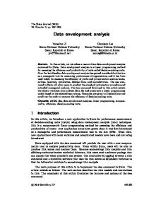
2.2.2.4 Allocative Efficiency When more than one input (and/or output) is part of health services delivery, health managers are interested in the appropriate mix of the inputs to serve patients so the organization can achieve efficiency. Let us consider three group practices, A, B and C, where two type professionals, physicians (P) and nurse practitioners (NP), provide health services. Furthermore assume that a physician’s time costs $100 per hour, whereas a nurse practitioner’s time costs $60 per hour. Let us suppose group practice A employs three physicians and one nurse practitioner; and that group practice B employs two physicians and two nurse practitioners, and finally that the group practice C employs three physicians and three nurse practitioners. Further assume that all group practices produced 500 equivalent patient visits during a week. Further assume that the practices are open for 8 h a day for 5 days a week (40 h). Input prices for the group practices are: Inputs for Group Practice A = [(3∗ 100) + (1∗ 60)]∗ 40 = $14, 400 Inputs for Group Practice B = [(2∗ 100) + (2∗ 60)]∗ 40 = $12, 800 Inputs for Group Practice C = [(3∗ 100) + (3∗ 60)]∗ 40 = $19, 200 Since the output is the same, evaluating the input mix for these two group practices per visit yields the following ratios: Group Practice A = 14, 400/500 = $28.80 Group Practice B = 12, 800/500 = $25.60 Group Practice C = 19200/500 = $38.40. Table 2.3 summarizes these calculations as follows: We can also illustrate these three group practices graphically on a production possibilities curves [pp] and [p p ] shown in Fig. 2.1. Group practices A and B lie on production possibilities curve [pp]. Because group practice C operates with a higher number of physicians and nurse practitioners when compared to practices A and B, the production possibilities curve [p p ] is in a higher position. Furthermore,

20

2 Performance Measurement Using Data Envelopment Analysis (DEA) Table 2.3 Allocative efficiency

Group practice

Physicians ($100/h)

Nurse practitioners ($60/h)

Input prices

Output: visits

Efficiency

Allocative efficiency

3 2 3

1 2 3

$14,400 $12,800 $19200

500 500 500

$28.80 $25.60 $38.40

0.889 1.000 0.667

A B C

p⬘ cC p cA

Physicians

3

$3.

cB

20

A

C p⬘

B

$38

2

.40

p $28

cC

$25

.80

.60

1

cA cB

0

1

2

3

Nurse Practitioners Fig. 2.1 Allocative efficiency

the cost per case is shown using cost lines cA ($28.80), cB ($25.60), and cC ($38.40), where Group Practice B is producing the services for $3.20 less per case compared to Group Practice A, as shown by cost line cA . Furthermore, group practice B is producing the services for $12.80 less per case when compared to Group Practice C. Comparing these costs, one can conclude that Group Practice A is 88.9% (25.60/28.80) efficient compared to Group Practice B. Similarly, the group practice C is 66.7% (25.60/38.40) efficient compared to Group Practice B. In addition, the group practice C is not only allocatively inefficient, but it is also technically inefficient, since it operates on a less efficient production possibilities curve [p p ]. This example illustrates the concept of allocative efficiency, where various combinations (mixes) of inputs and their prices will yield different efficiencies. We should also note that the contribution to outputs from each input might be different. In this example, while physicians can provide a full spectrum of services to the patients, nurse practitioners may be able to provide only a fraction, say, 70%, due

2.3 Data Envelopment Analysis (DEA)

21

to their limited training and other legal matters. This raises the concern of whether using physicians and nurse practitioners as equal professions in efficiency calculations is appropriate, or if a weighting scheme should be imposed to correctly assess the nurse practitioners contributions to the total output. These weights are not readily available in most instances; however, DEA can estimate these weights in comparative evaluations.

2.2.3 Effectiveness Measures Effectiveness in health care measured by outcomes or quality is of prime importance to many constituencies including patients, clinicians, administrators, and policy makers. Measuring the outcomes and quality is more problematic than efficiency measures. While inputs and outputs of the processes are relatively known to health care managers, multiple perspectives on outcomes and quality introduce additional practical difficulties in measurement. Although most hospitals report their inputs and outputs, until recently most outcome measures and quality measures, aside from mortality and morbidity statistics, were not reported on a systematic basis. The current quality reports from hospitals will be discussed in Chap. 7, and appropriate models will be developed to evaluate performance using both efficiency and effectiveness components.

2.3 Data Envelopment Analysis (DEA) DEA essentially forms a frontier using the efficient organizations. To illustrate the conceptualization of the DEA frontier, consider the performance ratios (Table 2.4) of the first five hospitals from the example in Chap. 1. Here we consider two inputs,

Table 2.4 Hospital performance ratios Provider ID

H1 H2 H3 H4 H5 H6 H7 H8 H9 H10

Nursing hours/inpatient admissions

Medical supplies/inpatient admissions

1.39 3.89 1.51 3.93 2.31 1.91 1.44 2.64 2.96 3.15

6.55 13.33 5.48 2.59 4.56 7.94 28.72 3.94 21.16 8.49

22

2 Performance Measurement Using Data Envelopment Analysis (DEA)

H7 (1.44, 28.72)

30.00 25.00

H9 (2.96, 21.16) 20.00

nc

yF

ron

tie

r

5.00 0.00 0.00

H2 (3.89, 13.33)

) .5 5 ,6

icie

(1 .3 9

10.00

Eff

1.00

H10 (3.15, 8.49) H5 (2.31, 4.56)

H6⬘

0.50

ff

Ine

y

nc icie

H6 (1.91, 7.94)

1

15.00

H

Medical Supplies per Admission

35.00

H3 (1.51, 5.48)

1.50

2.00

H4 (3.93, 2.59) H8 (264, 3.94) 2.50

3.00

3.50

4.00

4.50

Nursing Hours per Admission Fig. 2.2 Efficiency frontier

nursing hours and medical supplies, by dividing them by inpatient admissions; thus we obtain standardized usage of each input per inpatient admission. As we observed before, H1 and H4 are efficient providers with their respective mix of use on these two inputs. We also know that H3 was an efficient provider from other dimensions of the performance. Graphically, as shown in Fig. 2.2, we can draw lines connecting these three efficient providers. As can be observed, there are two more hospitals, H5 and H8, that fall on the boundaries drawn by these lines between H1 and H4. Hence, these lines connecting H1, H3, H5, H8 and H4 represent the efficiency frontier for this example and they are among the benchmark hospitals, because these hospitals have the lowest combinations of the inputs when both ratios taken into account. If we go back to the logic used to create the Table 2.4, where standardized efficiency ratios were calculated, we can observe that H1 and H4 received a standardized efficiency score of 1, and the other hospitals’ standardized efficiency scores were somewhere between 0 but less than 1 from one dimension of the performance. Here also in DEA, the efficient hospitals will receive a score of 1 and those that are not on the efficiency frontier line will be less than 1 but greater than 0. Although we cannot explain why H5 and H8 are on the frontier line based on the graphic (due to its two dimensions), it suffices to say that they also have the lowest combinations of the inputs when both ratios are taken into account. Later when we employ all inputs and outputs into the model, we will demonstrate with DEA why H5 and H8 receive a score of 1 and efficient. Hospital H6 compared to H1 and H3 is considered inefficient using these input combinations. The amount of inefficiency can be understood by examining the dashed line from the origin to H6. In this dashed line, the amount of inefficiency exists from the point it crosses the efficiency frontier to H6. So, for H6 to become efficient, it must reduce usage of both inputs proportionately to reach point H6 .

2.5 Basic Frontier Models

23

This is the normative power of DEA, where it can suggest how much improvement by each inefficient hospital is needed in each dimension of the resources.

2.4 Model Orientation As in ratio analysis, when we calculate efficiency output over input, and place emphasis on reduction of inputs to improve efficiency, in DEA analysis this is called input orientation. Input orientation assumes health care managers have more control over the inputs rather than arriving patients either for outpatient visit or admissions. Figure 2.2 is an example of an input-oriented model, where H6 must reduce its inputs to achieve efficiency. However, the reverse argument can be made that the health care managers, through marketing, referrals or by other means (such as reputation on quality of services) can attract patients to their facilities. This means they can augment their outputs given their capacity of inputs to increase their organization’s efficiency. Output augmentation to achieve efficiency in DEA is called output orientation. Output orientation will be further discussed in Sect. 2.11 below. Various DEA models have been developed to use either the input or output orientation, and these models emphasize proportional reduction of excessive inputs (input slacks) or proportional augmentation of lacking outputs (output slacks). However, there are also models where health care managers can place emphasis on both output augmentation and input reduction at the same time by improving output slacks and decreasing input slacks. These slack based-models are also called the additive model or non-oriented models in DEA literature and software.

2.5 Basic Frontier Models This book will consider various models that would be needed by health care managers. In this chapter, the basic frontier models will be presented. The following chapters will introduce the extensions to these basic models for those specific management needs in evaluation of health care organizational performance. There are various types of DEA models which may be used depending on the conditions of the problem on hand. Types of DEA models concerning a situation can be identified based on scale and orientation of the model. If one can assume that scale of economies do not change as size of the service facility increases, then constant returns to scale (CRS) type DEA models is an appropriate choice. The initial basic frontier model was developed by Charnes et al. (1978), known as the CCR model, using the last initials of the developers, but now widely known as the constant returns-to-scale (CRS) model. The other basic frontier model followed CRS as the variable returns-to-scale (VRS) model, though in this model one cannot assume that scale of economies do not change as size of the service facility increases. Figure 2.3 shows the basic DEA models based on returns to scale and model orientation. These models will be referred as “Envelopment Models.”

24

2 Performance Measurement Using Data Envelopment Analysis (DEA) CRS

CRS Input

VRS

VRS Input

CRS

CRS Output

VRS

VRS Output

Input

Orientation Output

Fig. 2.3 Basic DEA model classifications – envelopment models

2.6 Decision Making Unit (DMU) Organizations subject to evaluation in the DEA literature are called DMUs. For example, the hospitals, nursing homes, group practices, and other facilities that are evaluated for performance using DEA are considered as DMUs by many popular DEA software.

2.7 Constant Returns to Scale (CRS) Model The essence of the CRS model is the ratio of maximization of the ratio of weighted multiple outputs to weighted multiple inputs. Any health care organization compared to others should have an efficiency score of 1 or less, with either 0 or positive weights assigned to the inputs and outputs. Here, the calculation of DEA efficiency scores are briefly explained using mathematical notations (adapted from Cooper Seiford, and Tone, 2007). The efficiency scores (θo ) for a group of peer DMUs (j = 1 . . . n) are computed for the selected outputs (yrj , r = 1, . . . , s) and inputs (xij , i = 1, . . . , m) using the following fractional programming formula: s


Maximi ze θo =

r =1 m


u r yr o (2.1) v i xio

i=1 s


subject

r =1 to m


u r yr j ≤1

(2.2)

v i xi j

i=1

u r , v i ≥ 0 f or all r and i. In this formulation, the weights for the outputs and inputs, respectively, are ur and vi , and “o” denotes a focal DMU (i.e., each hospital, in turn, becomes a focal hospital

2.8 Example for Input-Oriented CRS DEA Model

25

when its efficiency score is being computed). Note that the input and output values, as well as all weights are assumed by the formulation to be greater than zero. The weights ur and vi for each DMU are determined entirely from the output and input data of all DMUs in the peer group of data. Therefore, the weights used for each DMU are those that maximize the focal DMU’s efficiency score. In order to solve the fractional program described above, it needs to be converted to a linear programming formulation for easier solution. Since the focus of this book is not on the mathematical aspects of DEA, an interested reader is referred to the appendix at the end of this chapter for more detail on how the above equations are algebraically converted to a linear programming formulation. Other DEA books listed in the references may also be consulted for an in-depth exposure. In summary, the DEA identifies a group of optimally performing hospitals that are defined as efficient and assigns them a score of one. These efficient hospitals are then used to create an “efficiency frontier” or “data envelope” against which all other hospitals are compared. In sum, hospitals that require relatively more weighted inputs to produce weighted outputs or, alternatively, produce less weighted output per weighted inputs than do hospitals on the efficiency frontier, are considered technically inefficient. They are given efficiency scores of strictly less than one, but greater than zero. Although DEA is a powerful optimization technique to assess the performance of each hospital, it has certain limitations which need to be addressed. When one has to deal with a significantly large numbers of inputs and outputs in the service production process and a small number of organizations are under evaluation, discriminatory power of the DEA will be limited. However, the analyst could overcome this limitation by only including those factors (input and output) which provide the essential components of the service production process, thus not distorting the outcome of the DEA results. This is generally done by eliminating one of pair of factors that are strongly positively correlated with each other.

2.8 Example for Input-Oriented CRS DEA Model Consider again the sample data presented in Chap. 1 with ten hospitals, two inputs and two outputs. Table 2.5 depicts the inputs and outputs according to formulation discussions presented above. As one can observe, peer hospitals (j = 1, . . . , 10) are listed for the selected inputs (xij , i = 1, 2) and outputs (yrj , r = 1, 2). The next step is to enter this information into the DEA Frontier solver, which is Excel add-on software. For information regarding installation of the software and other relevant details, readers are referred to “Running the DEAFrontier” section of the book at the end. The Excel sheet containing the data for DEA analysis required to be named “Data” is shown in Fig. 2.4 below. Please note that the first column is recognized as the hospital identifier, followed by two columns of inputs. Please also note that there is a blank column between

26

2 Performance Measurement Using Data Envelopment Analysis (DEA) Table 2.5 Hospital inputs and outputs

Hospitalsj 1 2 3 4 5 6 7 8 9 10

Inputs Nursing hours x1j Medical supplies ($) X2j 567 350 445 2200 450 399 156 2314 560 1669

2678 1200 1616 1450 890 1660 3102 3456 4000 4500

Outputs Inpatient Outpatient admissions Y1j visits Y2j 409 90 295 560 195 209 108 877 189 530

211 85 186 71 94 100 57 252 310 390

Fig. 2.4 DEAFrontier data setup

last input and first output. To run this model, open the Excel file shown in Fig. 2.4 and when the security warning comes up click on “Enable Macros” to activate the “DEAFrontier” add-on software. To run the model, click on the “DEAFrontier” button on the top banner shown in Fig. 2.4. Once the “DEAFrontier” is clicked, a pull-down menu appears with a choice of DEA models, as depicted in Fig. 2.5. To run the initial CRS model, choose the “Envelopment Model” option. This will prompt another screen to appear, as shown in Fig. 2.6. For model orientation select “Input-Oriented”, and for the returns to scale select “CRS”, then click OK to run the model. For certain DEA models another screen (shown in Fig. 2.6) will pop up asking if the second stage input and output slacks should be calculated. Click “OK”, and the resulting screen should correspond to Fig. 2.7.

2.8 Example for Input-Oriented CRS DEA Model

27

Fig. 2.5 DEAFrontier run

Fig. 2.6 DEAFrontier envelopment model

At this stage the health care manager can observe many results of the model to not only identify benchmark hospitals, but to also identify improvement strategies for those hospitals that are currently inefficient. The results are organized in various Excel sheets, as shown at the bottom banner in Fig. 2.7. These sheets include results of efficiency analysis in the “Efficiency” sheet, target inputs and outputs in the “Target” sheet, and the amount of

28

2 Performance Measurement Using Data Envelopment Analysis (DEA)

Fig. 2.7 Results of CRS input-oriented model

inefficiencies (slacks) in the “Slack” template. Next we will discuss the results from each of these templates.

2.9 Interpretation of the Results Figure 2.8 depicts the abridged version of the efficiency report, where efficiency scores of all ten hospitals are reported. This two-input and two-output model shows that six of the ten hospitals are efficient using these four dimensions. There is no surprise that H1, H3, H4 and H9 all received a score of 1 and are considered efficient. Furthermore, we observe that the efficiency of two additional hospitals, H5 and H8, could not be determined in ratio based analysis. However, with DEA using multiple inputs and outputs at the same time, we are able to discover them.

2.9.1 Efficiency and Inefficiency Hospitals H2, H6, H7 and H10 have scores of less than 1 but greater than 0, and thus they are identified as inefficient. These hospitals can improve their efficiency, or reduce their inefficiencies proportionately, by reducing their inputs (since we run an input-oriented model). For example, H2 can improve its efficiency by reducing certain inputs up to 38.5% (1.0–0.61541). Similarly, H6 and H10 can do so with

2.9 Interpretation of the Results

29

Fig. 2.8 Efficiency report for input-oriented model

approximately 25% input reduction. However, H7 is closer to an efficiency frontier, and needs only a 3.2% reduction in resources. This raises the question: which inputs are needed to be reduced by calculated proportions? These input reductions (or output augmentations in some cases) are called slacks.

2.9.2 Slacks Figure 2.9 comes from the “Slack” sheet of the DEA run results. Mathematical derivation of these slacks is presented in Appendix B of this chapter. Here, we observe that none of the efficient hospitals have any slacks. Slacks exist only for those hospitals identified as inefficient. However, slacks represent only the leftover portions of inefficiencies; after proportional reductions in inputs or outputs, if a DMU cannot reach the efficiency frontier (to its efficient target), slacks are needed to push the DMU to the frontier (target). It is interesting to note that H2 is required to reduce its nursing hours by approximately 12 h. However, despite the reduction in this input, it would not achieve efficiency. No other input can be reduced, thus, H2 should also augment its inpatient admission by 44.8. A similar situation in a different magnitude exists for H10. On the other hand, H6 cannot reduce any inputs, but must augment outpatient visits by 19.7 or 20 visits. Lastly, H7 should spend $2,309.19 less for medical supplies. Please note that these calculations are the results of Models two and four executed in succession or Model five, as explained in the appendices at the end of the chapter.

30

2 Performance Measurement Using Data Envelopment Analysis (DEA)

Fig. 2.9 Input and output slacks for input-oriented model

2.9.3 Efficient Targets for Inputs and Outputs We can summarize these findings further by examining the “Target” sheet. Here, for each hospital, target input and output levels are prescribed. These targets are the results of respective slack values added to outputs. To calculate the target values for inputs, the input value is multiplied with an optimal efficiency score, and then slack amounts are subtracted from this amount. For detailed formulations of these calculations, the reader is referred to Appendix B, Part 3. Figure 2.10 displays these target values. As the reader can observe, the target values for efficient hospitals are equivalent to their original input and output values. However, for the inefficient DMUs, in the CRS input-oriented DEA model, the  targets for input variables ( x io ) will comprise proportional reduction in the input variables by the efficiency score of the DMU minus the slack value, if any, given by the formula: ∗  x io = θ ∗ xio − si− i = 1, . . . , m (2.3) For example, the target calculations for nursing hours (NH) and medical supply (MS) inputs of Hospital H2 are calculated as follows: x N H,H 2 = θ ∗ x N H,H 2 − s N−∗H  x N H,H 2 = 0.61541∗ 350 − 12.03405  x N H,H 2 = 203.36022 

where 0.61541 comes from Fig. 2.8, 350 from Fig. 2.4, and 12.03405 from Fig. 2.9. The reader can confirm the results with Fig. 2.10. Similarly, target calculation of Medical Supply for H2 is: −∗ x M S,H 2 = θ ∗ x M S,H 2 − s M S x M S,H 2 = 0.61541∗ 1200 − 0  x M S,H 2 = 738.49462  

2.10 Input-Oriented Model Benchmarks

31

Fig. 2.10 Input and output efficient targets for input-oriented model

Again, the reader can confirm the result from Fig. 2.10. In an input-oriented model, efficient output targets are calculated as: ∗

y r o = yr o + si+



r = 1, . . . .s

(2.4)

In our ongoing example with H2, inpatient admissions (IA) and outpatient visits (OV) can be calculated as: ∗ 

∗

+ y I A,H 2 = y I A,H 2 + s I+A y O V,H 2 = y O V,H 2 + s O V   y I A,H 2 = 90 + 44.81183 y O V,H 2 = 85 + 0   y I A,H 2 = 134.81183 y O V,H 2 = 85.00 

The reader can confirm these results from Fig. 2.10 for Hospital H2. The other inefficient hospitals are calculated in the same manner.

2.10 Input-Oriented Model Benchmarks The “Efficiency” sheet in Fig. 2.7 provides more results shown in columns such as λ and RTS. These are subject to Chap. 4 and will be discussed in more detail with more foundation material presented. However, here we will explain the remaining information presented. These are the “Benchmarks” created by the DEA technique. Figure 2.11 is taken from portions of the results of the initial “Efficiency” sheet. Here, health care managers whose hospital is inefficient can observe the benchmark hospitals that they need to catch up to. Obviously efficient hospitals may consider themselves to be their own “benchmarks.” So, Benchmark for H1 is H1, for H3 is H3, and so on. However, for inefficient hospitals, their benchmarks are one or many of the efficient hospitals. For

32

2 Performance Measurement Using Data Envelopment Analysis (DEA)

Fig. 2.11 Benchmarks for input-oriented CRS model

example, a benchmark for H2 and H10 is H3 (observe that H3 is efficient). A benchmark for H6 and H7 are two hospitals, H1 and H3. This means, to become efficient, H6 and H7 must use a combination from both H1 and H3 (a virtual hospital) to become efficient. How much of H1 and how much of H3 (what combination) are calculated to achieve efficiency and reported next to each Benchmark hospital. These are λ weights obtained from the dual version of the linear program that is solved to estimate these values. Further formulation details are provided in Appendix A at the end of this chapter. For example, H7 will attempt to become like H1 more than H3 as observed from respective λ weights of H1 and H3 (λ1 = 0.237 vs. λ3 = 0.038).

2.11 Output-Oriented Models The essence of output orientation comes from how we look at the efficiency ratios. When we illustrated the input orientation we used the ratios in which inputs were divided by outputs. Hence we can do the opposite by dividing outputs by inputs, and create reciprocal ratios. Using the same inputs and outputs from Table 2.2 from Chap. 1, we can calculate these mirror ratios as shown in Table 2.6 below. The first two columns show two different outputs, inpatient admissions and outpatient visits, being divided by the same input, nursing hours. The higher ratio values here would mean better performance for the hospitals. H1 has the highest inpatient admissions per nursing hour compared to other providers, as can be observed from the first column. However, H4 has the highest outpatient visits per nursing hour as displayed in the second column. A graphical view of these measures is shown in Fig. 2.12, where H1, H3 and H9 have the highest combination of these ratios when considered together. Here, no other hospital can generate more outputs using the nursing hours as input. However, when other inputs are included in the model using DEA, we may discover other hospitals joining the efficiency frontier.

2.12 Output-Oriented CRS DEA Model

33

Table 2.6 Hospital performance ratios Provider ID

Inpatient admissions/ nursing hours

Outpatient visit/ nursing hours

0.72 0.26 0.66 0.25 0.43 0.52 0.69 0.38 0.34 0.32

0.37 0.24 0.42 0.03 0.21 0.25 0.37 0.11 0.55 0.23

H1 H2 H3 H4 H5 H6 H7 H8 H9 H10

ienc

y Fr

ontie

H7⬘

H3 (0.66, 0.42)

0.40

H10 (0.32, 0.23)

.37

,0

0.20

H6 (0.52, 0.25)

69

H2 (0.26, 0.24)

(0.

0.30

.72, 0

r

H1 (0

Effic 0.50

.37)

H9 (0.34, 0.55)

H7

H5 (0.43, 0.21)

)

Outpatient Visits per Nursing Hour

0.60

H8 (0.38, 0.11)

0.10

H4 (0.25, 0.03) 0.00 0.00

0.10

0.20

0.30

0.40

0.50

0.60

0.70

0.80

Inpatient Admissions per Nursing Hour Fig. 2.12 Efficiency frontier for output-oriented model

The reader should also note that H7, an inefficient hospital, can reach this outputoriented frontier by increasing its inpatient admissions and outpatient visits along the direction of the dashed line to H7 . The distance given by H7 −H7 defines the amount of inefficiency for H7.

2.12 Output-Oriented CRS DEA Model Using the similar steps in Sect. 2.8, this time we will select “Output-Oriented” from the Model Orientation box as shown in Fig. 2.13.

34

2 Performance Measurement Using Data Envelopment Analysis (DEA)

Fig. 2.13 Output-oriented envelopment model

Fig. 2.14 Results of output-oriented CRS model

Again answering “Yes” to the second stage slack calculations, we get the results shown in Fig. 2.14, which is similar to Fig. 2.7, however, the results report as output orientation.

2.13 Interpretation of Output-Oriented CRS Results Figure 2.15 depicts the abridged version of the efficiency report, where efficiency scores of all ten hospitals are reported. This two-input and two-output model shows six of the ten hospitals are efficient using these four dimensions in an outputoriented model.

2.13 Interpretation of Output-Oriented CRS Results

35

Fig. 2.15 Efficiency report for output-oriented model

2.13.1 Efficiency and Inefficiency Hospitals H2, H6, H7 and H10 have scores greater than 1; thus they are identified as inefficient in the output-oriented model. These hospitals can improve their efficiency, or reduce their inefficiencies proportionately, by augmenting their outputs (since we run an output-oriented model). For example, H2 can improve its efficiency by augmenting certain outputs up to 62.5% (1.62493–1.0). Similarly, H6 and H10 can do so with approximately 33% increase. However, H7 is closer to efficiency frontier, and needs only a 3.3% increase in outputs.

2.13.2 Slacks Figure 2.16 comes from the “Slack” sheet of the DEA run results. Here again we observe that none of the efficient hospitals have any slacks. Slacks exist only for those hospitals identified as inefficient. It is interesting to note that H2 is required to increase its inpatient admissions by 72.8 patients, after having proportionately increased this output by its efficiency score. However, despite the augmentation in this output, it still would not achieve efficiency. No other output can be increased. Thus, H2 should also reduce its nursing hours by 19.5 hours. A similar situation in a different magnitude exists for H10. On the other hand, H6 can augment its outpatient visits by 26. Lastly, H7 cannot augment its outputs at all, but could decrease its medical supplied cost by $2,384.24.

36

2 Performance Measurement Using Data Envelopment Analysis (DEA)

Fig. 2.16 Slacks of output-oriented CRS model

Fig. 2.17 Efficient targets for inputs and outputs for output-oriented CRS model

2.13.3 Efficient Targets for Inputs and Outputs Again, we can summarize these finding further by examining the “Target” sheet. For each hospital, target input and output levels are prescribed. These targets are the results of respective slack values added on to original outputs, and subtracted from original inputs. To calculate the target values for inputs, the input slacks are subtracted from the inputs. Targets for outputs are calculated by multiplying optimal efficiency scores by the outputs and then adding the slack values to that value. For a detailed formulation of these calculations, the reader is referred to Appendix C, Part 2. Figure 2.17 displays these target values. As the reader can observe, the target values for efficient hospitals are equivalent to their original input and output values. Health care managers should be cautioned that some of these efficiency improvement options (and the target values) may not be practical. Health care managers can opt to implement only some of these potential improvements at the present time due to their contracts with labor and supply chains and insurance companies.

2.15 Summary

37

Fig. 2.18 Benchmarks for output-oriented model

2.14 Output-Oriented Model Benchmarks Figure 2.14 displays portions of the results from initial “Efficiency” sheet. Here health care managers whose hospital is inefficient can observe the benchmark hospitals. As in the input-oriented model, the efficient hospitals for output-oriented model (Fig. 2.18) will consider themselves as their own “benchmark.” So, Benchmark for H1 is H1, for H3 is H3, and so on. On the other hand, for those inefficient hospitals the benchmarks are one or many of the efficient hospitals. For example, benchmark for H2 and H10 is H3 (observe that H3 is efficient). Benchmark for H6 and H7 are two hospitals, and these are H1 and H3. This means, to become efficient, H6 and H7 must use a combination of H1 and H3 (a virtual hospital) to become efficient. How much of H1 and how much of H3 are calculated and reported next to each benchmark hospital? These are λ weights obtained from the dual version of the linear program that is solved to estimate these values. Further formulation details are provided in the appendix. For example, H7 will attempt to become like H1 more than H3, as observed from respective λ weights of H1 and H3 (λ1 = 0.244 vs. λ3 = 0.039).

2.15 Summary This chapter introduced the basic efficiency concepts and DEA technique. The model orientation and returns to scale are basic concepts that help health care managers in identifying what type of DEA model they should use. We discussed only input and output-oriented CRS models in this chapter.

38

2 Performance Measurement Using Data Envelopment Analysis (DEA)

Appendix A A.1 Mathematical Details Fractional formulation of CRS model is presented below: Model 1 s


Maximi ze θo =

u r yr o v i xio

i=1

s
=1 subject to r
m

ur , vi ≥ 0

r =1 m


u r yr j v i xi j

≤1

i=1

f or all r and i.

This model can be algebraically rewritten as: Maximi ze θo = subject to

s
r =1

s
r =1

u r yr o

u r yr j ≤

m


v i xi j

i=1

with further manipulations we obtain the following linear programming formulation: Model 2 s
u r yr o Maximi ze θo = r =1

Subject to: s
r =1 m


u r yr j −

v i xio = i=1 ur , vi ≥ 0

m


v i xi j ≤ 0

j = 1, . . . .n

i=1

1

A.2 Assessment of the Weights To observe the detailed information provided in Fig. 2.7, such as benchmarks and their weights (λ), as well as λ leading to returns to scale (RTS) assessments, a dual version of the Model 2 is needed. The dual model can be formulated as:

B.1 Mathematical Details for Slacks

39

Model 3 Minimi ze θo Subject to: n
j=1 n


λ j xi j ≤ θ xio λ j yr j ≥ yr o

j=1

λj ≥ 0

i = 1, . . . , m r = 1, . . . , s

j = 1, . . . , n.

In this dual formulation, Model 3, the linear program, seeks efficiency by minimizing (dual) efficiency of a focal DMU (“o”) subject to two sets of inequality. The first inequality emphasizes that the weighted sum of inputs of the DMUs should be less than or equal to the inputs of focal DMU being evaluated. The second inequality similarly asserts that the weighted sum of the outputs of the non-focal DMUs should be greater than or equal to the focal DMU. The weights are the λ values. When a DMU is efficient, the λ values would be equal to 1. For those DMUs that are inefficient, the λ values will be expressed in their efficiency reference set (ERS). For example, observing Fig. 2.7, H7 has two hospitals in its ERS, namely H1 and H3. Their respective λ weights are reported as λ1 = 0.237 and λ3 = 0.038.

Appendix B B.1 Mathematical Details for Slacks In order to obtain the slacks in DEA analysis, a second stage linear programming model is required to be solved after the dual linear programming model, presented in Appendix A, is solved. The second stage of the linear program is formulated for slack values as follows as: Model 4 m s

si− + sr+ Maximi ze n
j=1 n
j=1

r =1

i=1

λ j xi j + si−

=

θ∗x

io

λ j yr j − sr+ = yr o

λj ≥ 0

i = 1, . . . , m r = 1, . . . , s

j = 1, . . . , n ∗

Here, θ is the DEA efficiency score resulted from the initial run, Model Two, of the DEA model. Here, si− and sr+ represent input and output slacks, respectively. Please note that the superscripted minus sign on input slack indicates reduction, while the superscripted positive sign on output slacks require augmentation of outputs.

40

2 Performance Measurement Using Data Envelopment Analysis (DEA)

In fact, Model Two and Model Four can be combined and rewritten as: Model 5: Input-Oriented CRS Model  m s
−
Minimi ze θ − ε si + sr+ n
j=1 n
j=1

r =1

i=1

λ j xi j + si−

= θ xio

λ j yr j − sr+ = yr o

λj ≥ 0

i = 1, . . . , m r = 1, . . . , s

j = 1, . . . , n

The ε in the objective function is called the non-Archimedean, which is defined as infinitely small, or less than any real positive number. The presence of ε allows a minimization over efficiency score (θ) to preempt the optimization of slacks, si− and sr+ . Model Five first obtains optimal efficiency scores (θ∗ ) from Model Two and calculates them, and then obtains slack values and optimizes them to achieve the efficiency frontier.

B.2 Determination of Fully Efficient and Weakly Efficient DMUs According to the DEA literature, the performance of DMUs can be assessed either as fully efficient or weakly efficient. The following conditions on efficiency scores and slack values determine the full and weak efficiency status of DMU: Condition




θ∗

All s− i

all s+ r

Fully efficient Weakly efficient

1.0 1.0

1.0 1.0

0 At least one si− = 0

0 At least one sr+ = 0

When Models Two and Four run sequentially (Model Five), weakly efficient DMUs cannot be in the efficient reference set (ERS) of other inefficient DMUs. However, if only Model Two is executed, then weakly efficient DMUs can appear in the ERS of inefficient DMUs. The removal of weakly inefficient DMUs from the analysis would not affect the frontier or the analytical results.

B.3 Efficient Target Calculations for Input-Oriented CRS Model In input-oriented CRS models, levels of efficient targets for inputs and outputs can be calculated as follows: Inputs: x io = θ ∗ xio − si−∗ i = 1, . . . , m  Outputs: y r o = yr o + si+∗ r = 1, . . . , s 

C.2 Efficient Target Calculations for Output-Oriented CRS Model

41

Appendix C C.1 CRS Output-Oriented Model Formulation Since Model Five, as defined in Appendix B, combines the needed calculations for input-oriented CRS model, we can adapt the output-oriented CRS model formulation using this fully developed version of the model. Model 6: Output-Oriented CRS Model  m s
−
+ Maximi ze φ − ε si + sr n
j=1 n
j=1

i=1

λ j xi j + si−

= xio

λ j yr j − sr+ = φyr o

λj ≥ 0

r =1

i = 1, . . . , m i = 1, . . . , s

j = 1, . . . , n

The output efficiency is defined by φ. Another change in the formula is that the efficiency emphasis is removed from input (first constraint) and placed into output (second) constraint.

C.2 Efficient Target Calculations for Output-Oriented CRS Model In output-oriented CRS models, levels of efficient targets for inputs and outputs can be calculated as follows: Inputs: x io = xio − si−∗ i = 1, . . . , m  Outputs: y r o = φ ∗ yr o + si+∗ r = 1, . . . , s. 

http://www.springer.com/978-0-387-75447-5