1
Radio Tomographic Imaging with Wireless Networks Joey Wilson Neal Patwari University of Utah
Abstract—Radio Tomographic Imaging (RTI) is an emerging technology for imaging passive objects (objects that do not carry a transmitting device) with wireless networks. This paper presents a linear model for using received signal strength (RSS) measurements to obtain images of moving objects. A Gaussian noise model is assumed, the accuracy of which is examined through a measurement campaign. A maximum a posteriori (MAP) estimator is derived as an image reconstruction algorithm, and an experimental implementation of RTI is presented with resultant images.
I. I NTRODUCTION Radio tomographic imaging (RTI) is an emerging application which offers a new way to image passive objects in buildings and outdoor environments using received signal strength (RSS). The reduction in costs for radio frequency integrated circuits (RFICs) and advances in peer-to-peer data networking, have made realistic the use of hundreds or thousands of simple radio devices in a single RTI deployment. We describe in this paper an imaging system which has power that increases as Metcalf’s Law with the number of nodes, and suggest using low-complexity devices to enable large numbers of nodes. Radio tomography takes the advantages of two well-known and widely used types of imaging systems. First, radar systems transmit RF probes and receive echoes caused by the objects in an environment [1]. A delay between transmission and reception indicates a distance to a scatterer. Phased array radars also compute an angle of bearing. Such systems image an object in space based on reflection and scattering. Secondly, computed tomography (CT) methods in medical and geophysical imaging systems send signals along many different paths through a medium and measure the magnitude and phase of the transmitted signal. The measurements on many paths is used to compute an estimate of the spatial field of the transmission parameters throughout the medium [2]. Radio tomography is also a transmission-based imaging method which measures received signals on many different paths through a medium, however, it does so at radio frequencies similar to radar systems. Tomography at radio frequencies across large, cluttered environments experiences two major additional complications compared to typical CT systems. • RTI systems measure only signal magnitude. Medical tomographic systems have motorized sensors which are used to measure phase differences at different positions. The high expense and deployment complexity involved
Fig. 1. An illustration of an RTI network. Each node broadcasts to the others, creating many projections that can be used to reconstruct an image of objects inside the network area.
in providing such a capability makes it incompatible with the low-cost application space we target with RTI. • The use of RF as opposed to much higher frequency EM waves (e.g., x-rays), introduces significant non-line-ofsight (NLOS) propagation in the transmission measurements. Signals in standard commercial wireless bands do not travel in just the line-of-sight (LOS) path, and instead propagate in many directions from a transmitter to a receiver. Despite the difficulties of using RF, there is a major advantage: RF signals can travel through obstructions such as walls, trees, and smoke, while optical or infrared imaging systems cannot. RF imaging will also work in the dark, where video cameras will fail. Even for applications where video cameras could work, privacy concerns may prevent their deployment. An RTI system provides current images of the location of people and their movements, but cannot be used to identify a person. A. Applications One main application of RTI is to reduce injury for correctional and law enforcement officers; many are injured each year because they lack the ability to detect and track offenders through building walls [3]. By showing the locations
2
of people and walls within a building during hostage situations, during building fires, or after an earthquake, RTI can help law enforcement and emergency responders to know where they should focus their attention and recovery efforts. Another application is in automatic monitoring and control in ‘smart’ homes and buildings. Some building control systems detect motion in a room and use it to control lighting, heating, air conditioning, and even noise cancellation [4]. RTI systems can further determine how many people are in a room and where they are located, providing more precise control. Generally RTI has application in security and monitoring systems for indoor and outdoor areas. For example, existing security systems are trip-wire based or camera-based. Tripwire systems detect when a person crosses a boundary, but do not track the person when they are within the area. Cameras are ineffective in the dark. An RTI system could serve both as a trip-wire, alerting when intruders enter into an area, and tracking where are at all times while they are inside, regardless of availability of lighting or obstructions.
Recent research has also used measurements of path loss on 802.11 WiFi links to detect and locate a person’s location [13]. Experiments in [13] demonstrate the capability of a detector based on the change in signal strength variance to detect and to identify which of four links a person is obstructing. Our approach is not based on point-wise detection. Instead, we use tomographic methods to estimate an image of the change in the attenuation as a function of space, and use the image estimate for the purposes of tracking. In our previous research, we have performed an experimental test of RTI in an empty indoor environment [14] as part of a larger study of how to model link shadowing. This paper presents a formal derivation and a real-time application of the maximum a posteriori (MAP) tomographic image reconstruction estimator, which has not been presented in prior work. Further, past work explored neither the noise model nor realtime tracking, as is done in this paper.
B. Related Work RF-based imaging has been dominated in the commercial realm by ultra-wideband (UWB) based through-the-wall (TTW) imaging devices, including include Time Domain’s Radar Vision [5], Cambridge Consultants’ Prism 200 [6] and Camero Tech’s Xaver800 [7]. Each device is a phased array of radars which transmit UWB pulses and then record the return echoes and estimate a range and bearing. These devices are accurate close to the device, but inherently suffer from accuracy and noise issues at long range due to monostatic radar losses and large bandwidths, and involve only one device. Some initial attempts [8] allow 2-4 of these high-complexity devices to collaborate to improve coverage. In comparison, in this paper we discuss using dozens to hundreds of low-capability collaborating nodes, which measure transmission rather than scattering and reflection. Further, UWB uses extremely wide RF bandwidth, which will limit its application to commercial, non-emergency applications. Our paper investigates using radios with relatively small bandwidths. To emphasize the small required bandwidth compared to UWB, some relevant research is being called “ultranarrowband” (UNB) radar [9], [10], [11]. These systems propose using narrowband transmitters and receivers deployed around an area to image the environment within that area. Measurements are phase-synchronous at the multiple sensors around the area. Such techniques have been applied to detect and locate objects buried under ground using what are effectively a synthetic aperture array of ground-penetrating radars [12]. Experiments have been reported which measure a static environment while moving one transmitter or one receiver [11], and measure a static object on a rotating table in an anechoic chamber in order to simulate an array of transmitters and receivers at many different angles [11], [12], [9]. Because in this paper we use low complexity, non-coherent sensors, we can deploy many sensors and image in real time, enabling the study of tracking moving objects. We present experimental results with many devices in real-world, cluttered environments.
This paper explores in detail the use of RF path losses on links between many pairs of nodes in a wireless network in order to image the changes in attenuation that occur within the area of their deployment. We refer to this problem as radio tomographic imaging (RTI). In general, when an object moves into the area of deployment, we expect that links which pass through that object will, on average, experience higher shadowing losses. We explore the inverse perspective, that is, the use of the measurement of additional path losses on multiple, intersecting links to image the attenuation within the area and infer the location of an attenuating object. Section II presents a linear model relating RSS measurements to the moving attenuation occuring in a network area, and investigates statistics for noise in dynamic multipath environments. Section III derives the MAP solution for obtaining an attenuation image using Gaussian prior assumptions. Section IV describes the setup of an actual RTI experiment, the parameters used, and the resultant images.
C. Overview
II. M ODEL A. Algebraic Formulation When wireless nodes communicate, the radio signals pass through the physical area of the network. Objects within the area absorb, reflect, diffract, or scatter some of the transmitted power. The goal of an RTI system is to determine a vector x ∈ RN that describes the amount radio power attenuation occurring due to physical objects within N voxels of a network region. Since voxels locations are known, RTI allows one to know where attenuation in a network is occurring, and therefore, where passive objects are located. If K is the number of nodes in the RTI network, then the 2 total number of unique two-way links is M = K 2−K . Any pair of nodes is counted as a link, whether or not communication actually occurs between the two nodes. The averaged two-way signal strength R of a particular link is dependent on: • Pt : Transmitted power. • Ss : Shadowing loss due to static objects that attenuate the signal.
3
Sm : Shadowing loss due to moving objects that attenuate the signal. • F : Fading gain that occurs from constructive and destructive interference of narrow-band signals in multipath environments. • Ld : Large-scale path loss due to the distance between two nodes. • La : Static losses due to antenna patterns, device inconsistencies, etc. • ν: Noise. Mathematically, the received signal strength (in dB) is described as •
R = Pt − Ld − La − Ss − Sm + F − ν
(1)
This paper is concerned with imaging motion in an RTI network, not static objects. If all static terms are grouped into one variable Rs = Pt − Ld − La − Ss and the fading effects are grouped with the noise as n = F + ν, (1) can be written as y = Rs − R = Sm + n. (2) Rs can be determined using RSS measurements when no motion is occurring within the network, or by taking an average of previous measurements. A simple calibration procedure for determining this value is described in Section IV. If images of static attenuation are desired, the shadowing terms can be grouped, but the difficulty of determining individual losses arises. The shadowing loss Sm can be approximated as a weighted sum of the changed attenuation that occurs in each voxel. Since the contribution of each voxel to the attenuation of a link is different for each link, a weighting is applied. Mathematically, this is described for link i as Sm (i) =
N X
wij xj .
(3)
j=1
If a link does not “cross” a particular voxel, that voxel is removed by using a weight of zero. For example, Fig. 2 is an illustration of how a direct LOS link might be weighted in a non-scattering environment. In Section IV, an ellipse is used as a simple mechanism to determine LOS weighting. If all links in the network are considered simultaneously, the system of RSS equations can be described in matrix form as y = Wx + n (4) where y is the vector of all difference RSS measurements, n is a noise vector, W is the weighting matrix, and x is the attenuation image to be estimated, all measured in decibels (dB). W is of dimension M × N , with each column representing a single voxel, and each row describing the weighting of each voxel for that link. B. Noise Statistics To complete the model, the statistics of the noise vector n in (4) must be examined. The noise is dependent on the accuracy of the linear model, and may vary depending on how the received signal strength is calculated.
Fig. 2. An illustration of a single link in an RTI network that travels in a direct LOS path. The signal is absorbed by objects as it crosses the area of the network in a particular path. The darkened voxels represent the image areas that have a non-zero weighting for this particular link.
In multipath environments, fading plays a significant role in the received signal strength of a wireless link. Small changes in the phase of a few multipath components, even due to motion outside of the network area or small changes in node position, can dramatically impact the measured RSS. Fading effects are therefore a significant part of the noise statistics. In this paper, a Gaussian noise model is assumed. Although this is certainly an approximation, the benefits of using Gaussian noise are evident when deriving a estimation procedure for the image. Gaussian noise leads to a tractable, closedform solution, and makes a theoretical analysis of estimation variance much simpler. More accurate noise modeling for RTI networks in multipath environments is a topic for future research. To measure the accuracy of the Gaussian noise assumption, RSS measurements from multiple network links in indoor environments were examined. These links were placed in locations with object motion occurring in the surrounding areas so that fading effects would be present. Objects were not allowed to cross the LOS paths of the links to avoid confusing the effects of shadowing (the parameters being estimated in the RTI model) with the noise statistics. For each network deployment, many RSS measurements were taken. The mean was removed and the variance normalized for each batch to reduce the deployment dependent effects, then merged for comparison with a theoretical distribution. Fig. 3 is a quantile-quantile plot comparing the RSS measurements with a theoretical standard normal distribution. The measured data does not deviate significantly from a standard normal distribution until after the second standard deviation, indicating that a gaussian noise model provides a reasonable level of accuracy. III. I MAGE R ECONSTRUCTION An image reconstruction algorithm estimates the image vector x from path loss projections contained in the data vector
4
Finally, taking the gradient with respect to x and setting equal to zero results in the MAP estimator
Measured Data Quantile
10
2 −1 T ˆxM AP = (WT W + C−1 W y. x σN )
5
By incorporating prior assumptions about the image, the singularity of the inverse shown in (12) is removed by adding the inverse of the prior covariance, weighted by the noise variance. If noise is very high, the solution is weighted closer towards the a priori information. When noise variance is low, the effect of the prior information plays less of a roll. The MAP solution is simply a linear projection of the measurement data, which is possible because the model is linear and all parameter and data models are assumed to be normal [15]. It can be re-written as
0 −5 −10 −4 −3 −2 −1 0 1 2 3 Theoretical Normal Quantile
4
Fig. 3. A q-q plot comparing a standard normal distribution with that of RSS measurements taken in indoor environments with surrounding motion.
y. Many inverse problems, include the RTI formulation, are illposed, and some form of regularization must be incorporated to achieve reasonable results. Here, a Bayesian approach to image reconstruction is presented, but other algorithms for algebraic models exist [2]. If it is assumed that noise is i.i.d. Gaussian, the maximum likelihood (ML) estimator results in the least squares solution ˆ xM L = (WT W)−1 WT y.
(5)
In this case, the matrix (WT W) is almost always singular. The ML solution, although optimal in the sense of least squared error, amplifies the noise to such an extent that the solution becomes meaningless. To regularize the problem, a priori information about the image vector is incorporated, and the maximum a posteriori (MAP) formulation is used instead of ML. ˆ xM AP = arg max P (x|y) = arg max P (y|x)P (x). x x
(6)
To derive a MAP estimator, it can be assumed that x is a zero-mean gaussian random field with covariance matrix Cx . Then −1 T 1 1 P (x) = p e− 2 (x Cx x) (7) N (2π) |Cx | and P (y|x) =
1 2 )M/2 (2πσN
e
−
1 2σ 2 N
||y−Wx||2
(8)
Since the log function is monotonic, the log likelihood can be used to simplify the MAP derivation as follows. ˆ xM AP
= =
arg max ln P (x|y) x arg max ln P (y|x) + ln P (x) x
(9) (10)
The minimization used in the MAP estimator is over x, so any terms that do not contain it may be dropped. Plugging (7) and (8) into (10) and replacing the argmax function with argmin by inverting the sign results in 1 1 ˆ xM AP = arg min 2 ||y − Wx||2 + xT C−1 x x. x 2σN 2
(12)
(11)
ˆxM AP
=
Πy
Π
=
2 −1 T (WT W + C−1 W . x σN )
(13)
Since the projection matrix Π only needs to be calculated once, MAP reconstruction is very suitable for realtime RTI implementation. IV. E XPERIMENTAL R ESULTS An experiment using twenty eight “Telosb” wireless nodes by Crossbow (2.4 GHz) was deployed in a large indoor room. Furniture, walls, moving people, and other building structures provided a rich multipath environment for testing. The nodes were set up in a square network with a length of 14 feet on each side, totaling 196 square feet. Each side of the square contained eight nodes separated by two feet, similar to the network depicted in Fig. 1. An ellipse with foci at each node location is used to determine the weighting for each link in the network. If a particular pixel falls inside the ellipse, it is weighted as nonzero, while all pixels outside the ellipse are set to weight zero. Additionally, the weight for each pixel is normalized by the link length. � 1 1 if dij (1) + dij (2) < d + λ (14) wij = √ 0 otherwise d where d is the distance between the two nodes, dij (1) and dij (2) are the distances from the center of voxel j to the node locations for link i, and λ is a parameter describing the width of the ellipse. The a priori covariance matrix Cx was created using an exponential spatial decay [Cx ]kl = σx2 e−dkl /δc
(15)
where dkl is the distance from pixel k to pixel l, δc is a “space constant” correlation parameter that determines the amount of “smoothness” of the resultant image, and σx2 is the variance at each pixel. High values for δc results in smoother images, but also reduces detail. While an exponential spatial covariance is easily calculated and tunable, other models for prior covariance could possibly be used. To image motion, the static measurment vector {Rs } as described in Section II must be determined. This the instantaneous measurements is subtracted from this vector to remove
5
Parameter N ∆p Nc
Value 28 .6 2000
Description Number of nodes Normalized pixel width (m) Number of calibration frames
TABLE I S YSTEM SETUP USED TO OBTAIN RESULTS SHOWN IN F IG . 4 AND F IG . 5.
Parameter λ δc σx2 2 σn
Value .02 4 .4 10
Description Width of weighting ellipse in (14) (m) Pixel correlation constant in (15) (m) Pixel variance in (15) (dB)2 Noise variance in (12) (dB)2
TABLE II R ECONSTRUCTION PARAMETERS USED TO OBTAIN RESULTS SHOWN IN F IG . 4 AND F IG . 5.
effects of static objects and deployment dependent losses. To calibrate the system and obtain the static measurements, the network is assumed to be stationary and vacant from moving objects. The signal strength from each link taken Nc times and is averaged over the entire calibration period. This measurement vector is stored for difference comparison when the system is in use. The images in Fig. 4 and Fig. 5 show the results of the implemented RTI system using MAP reconstruction (12). Table II lists the model parameters used to obtain the results in these figures. An outdoor deployment of an RTI network was also tested. Experiments demonstrate that it is possible to obtain the same “quality” of image over a larger area with the same number of nodes in outdoor environments. This is most likely due to the reduction in multipath effects, and future research will continue to investigate these observations. V. C ONCLUSION Radio Tomographic Imaging (RTI) is a method of imaging passive objects within a wireless network. This paper presented a linear model relating signal strength (RSS) measurements to attenuation occuring within spatial voxels of a network area. A measurement campaign was performed to validate a Gaussian assumption for the noise vector statistics. These measurements were taken indoors when people were moving near the links, capturing the effects of fading. Resultant quantile-quantile plots indicate that a Gaussian noise assumption is reasonable, but future work will entail the use of more complicated noise models. RTI is an ill-posed inverse problem, and regularization must be incorporated to obtain usable results. In this study, the image is assumed to be Gaussian, and a MAP estimator is used for image reconstruction. The MAP estimator provides a simple and closed-form solution which is mathematically simple and suitable for real-time implementation. Other forms of inverse problem regularization, prior assumptions, and image reconstruction algorithms topics for future research. An implementation of an RTI system using 28 nodes operating at 2.4 GHz. Results show that the system is effective in creating attenuation images of humans standing in areas on the order of hundreds of square feet.
Finally, images created via RTI provide a natural framework to track targets that move within a wireless network. R EFERENCES [1] M. Skolnik, Introduction to radar systems. McGraw Hill Book Co., 1980. [2] A. C. Kak and M. Slaney, Principles of Computerized Tomographic Imaging. The Institute of Electrical and Electronics Engineers, Inc., 1988. [3] A. Hunt, C. Tillery, and N. Wild, “Through-the-wall surveillance technologies,” Corrections Today, vol. 63, July 2001. [4] D. Estrin, R. Govindan, and J. Heidemann, “Embedding the internet,” Communications of the ACM, vol. 43, pp. 38–41, May 2000. [5] “Time Domain Corp., Radar Vision.” [6] “Cambridge Consultants, Prism 200 through wall radar.” [7] “Camero Tech, Xaver800.” [8] A. R. Hunt, “Image formation through walls using a distributed radar sensor network,” in SPIE Conference on Sensors, and Command, Control, Communications, and Intelligence (C3I) Technologies for Homeland Security and Homeland Defense IV, vol. 5778, pp. 169–174, May 2005. [9] S. L. Coetzee, C. J. Baker, and H. Griffiths, “Narrow band high resolution radar imaging,” in IEEE Conf. on Radar, pp. 24–27, April 2006. [10] H. D. Griffiths and C. J. Baker, “Radar imaging for combatting terrorism,” in NATO Advanced Study Institute Imaging for Detection and Identification, pp. 1–19, July/August 2006. [11] M. C. Wicks, B. Himed, L. J. E. Bracken, H. Bascom, and J. Clancy, “Ultra narrow band adaptive tomographic radar,” in 1st IEEE Intl. Workshop Computational Advances in Multi-Sensor Adaptive Processing, Dec. 2005. [12] M. C. Wicks, “Rf tomography with application to ground penetrating radar,” in 41st Asilomar Conference on Signals, Systems and Computers, pp. 2017–2022, Nov. 2007. [13] M. Youssef, M. Mah, and A. Agrawala, “Challenges: device-free passive localization for wireless environments,” in MobiCom ’07: Proc. 13th ACM Int’l Conf. Mobile Computing and Networking, pp. 222–229, Sept. 2007. [14] N. Patwari and P. Agrawal, “Effects of correlated shadowing: Connectivity, localization, and RF tomography,” in ACM/IEEE Information Processing in Sensor Networks (IPSN), April 2008. [15] A. Tarantola and B. Valette, “Generalized nonlinear inverse problems solved using the least squares criterion,” Reviews of Geophysics and Space Physics, vol. 20, pp. 219–232, May 1982.
6
(a)
(b)
Fig. 4. (a) Photo of an 28-node RTI system with one person inside the network boundaries. (b) RTI results using MAP reconstruction for the setup shown in (a). The bright spot reveal the human’s location within the network region. Only one measurement for each link was used to construct the image.
(a)
(b)
Fig. 5. (a) Photo of an 28-node RTI system with two people inside the network boundaries. (b) RTI results using MAP reconstruction for the setup shown in (a). The bright spots reveal the humans’ location within the network region. Only one measurement for each link was used to construct the image.