RID: Radio Interference Detection in Wireless Sensor Networks Gang Zhou, Tian He, John A. Stankovic,Tarek Abdelzaher Department of Computer Science University of Virginia, Charlottesville 22903 {gzhou,tianhe,stankovic,zaher}@cs.virginia.edu Abstract— In wireless sensor networks, many protocols assume that if node A is able to interfere with node B’s packet reception, then node B is within node A’s communication range. It is also assumed that if node B is within node A’s communication range, then node A is able to interfere with node B’s packet reception from any transmitter. While these assumptions may be useful in protocol design, they are not valid, according to the real experiments we conducted in MICA2 platform. For a strong link that has a high packet delivery ratio, the interference range is observed smaller than the communication range, while for a weak link that has a low packet delivery ratio, the interference range is larger than the communication range. So using communication range information alone is not enough to design real collisionfree media access control protocols. This paper presents a radio interference detection protocol (RID) and its variation (RID-B) to detect run-time radio interference relations among nodes. The interference detection results are used to design real collision-free TDMA protocols. With extensive simulations in GlomoSim, and with sensor network application scenarios, we observe that the TDMA which uses the interference detection results has 100% packet delivery ratio, while the traditional TDMA has packet loss up to 60%, in heavy load. In addition to the scheduling-based TDMA protocols, we also explore the application of interference detection on contention-based MAC protocols.

I. INTRODUCTION Wireless sensor networks (WSN) is an emerging technology that has a wide range of potential applications [1], including environment monitoring, smart houses, remote medical systems, sheep shepherding, and intrusion detection. Recent work [2][3][4][5][6] found that radio communication in wireless sensor networks (WSN) differs significantly from traditional Mobile Ad-Hoc Networks (MANET). For example, when node C’s signal can interfere with node A’s signal, preventing A’s signal from being received at node B, it’s usually assumed that node B must be within node C’s communication range and there is communication connectivity from C to B. We name this assumption the interference-connectivity assumption, which is widely used to design collision-free Media Access Control (MAC) protocols [7][8]. However, from our experiments on the MICA2 platform, we find that this interference-connectivity assumption is not valid. In actuality, a node can interfere with another node even if it is beyond its communication range. In our experiments we show that when the receiver is within, but close to the edge of the transmitter’s radio range, (referred to as a weak link), the transmitter’s signal is easily interfered with at the receiver by another node which has no connectivity with the receiver. Such

experiments are repeated several times and it is always found that the interference-connectivity assumption is violated. The interference-connectivity assumption assumes that interference always comes from connectivity. Another assumption, the connectivity-interference assumption, assumes that connectivity always leads to interference. The connectivityinterference assumption was firstly addressed in [9] and is described as follows: when two transmitters, A and B, both have connectivity to a receiver C and transmit simultaneously, a collision occurs, the data is corrupted and neither packet is received correctly. Our experiments confirm the observation in [9] that the connectivity-interference assumption is not always maintained. In other words in spite of the logical interference, one packet may be received while the other is corrupted. We observe that this assumption is usually violated in the case of strong links, that is, when the transmitter is close to the receiver and has a very strong signal that dominates the interfering signal. Without these assumptions between connectivity and interference, it’s extremely challenging to design collision-free MAC protocols. In this paper, the idea of radio interference detection at run-time is put forth, for the first time, to design real collision free MAC protocols that don’t depend on these nonrealistic assumptions. Our solutions obtain the interference relations among nodes to assist in achieving real collision-free packet delivery. The design of the radio interference detection protocol, RID, is presented. A lightweight version, the RIDBasic (RID-B), is also presented. Extensive simulations using sensor network scenarios are conducted to compare the performance of TDMA and TDMA-RID-B (TDMA with RID-B support). The performance evaluation shows that traditional TDMA can have up to 60% packet loss in heavy-loaded networks, while TDMA-RID-B can maintain 100% packet delivery ratio. The rest of this paper is organized as follows: in Section II, experimental observations of radio interferences in the MACA2 platform are presented. Then in Section III, the radio interference detection protocol, RID, and its variation, RIDB, are explained. In Section IV, extensive performance evaluations of TDMA and TDMA-RID-B, in which the TDMA scheduling is based on RID-B’s interference detection result, are analyzed. In addition, it is also explained how to use RID on contention-based MAC protocols. In Section VI, related work is analyzed, and finally in Section VII, conclusions are

given and future work is pointed out. II. EXPERIMENTS ON RADIO INTERFERENCE In this section, we present experimental results collected in an outdoor environment with MICA2 motes. From these experiments, it is confirmed that radio interferences are ubiquitous phenomena. It is also observed that for a weak link that has a low packet delivery ratio, the interference range is larger than the communication range, while for a strong link that has a high packet delivery ratio, the interference range is smaller than the communication range. A. Experimental Setup For each experiment, three MICA2 motes are used. One MICA2 mote is used as the transmitter, and another MICA2 mote is used as the receiver, and the third one is used as the jammer, whose transmission is synchronized with that of the transmitter to generate possible interference. The carrier sensing and backoff operations in the MAC layer are disabled to ensure packets are simultaneously sent out by the jammer and the transmitter. The radio interferences are reflected by the changing packet delivery ratios.

r2

r1

R

Move

T

J

(a) A Weak Link From T to R

r2

r1

R

Move

T

J

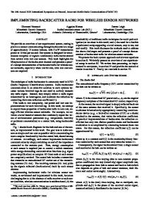
(b) A Strong Link From T to R Fig. 1.

Empirical Experiment Setting

All experiments are conducted in an open parking lot late at night, in order to separate possible influence from people and moving cars on the radio interference measurements. In the experiment, as Figure 1 illustrates, the transmitter T and receiver R are fixed in positions, and jammer J moves along the line determined by the positions of the transmitter and the receiver. The jammer is tried at different positions along the line to observe different degrees of interferences, and interference observations in different directions are measured as well.

In the experiments, two kinds of links are used, strong links and weak links. The setting of a weak link case is presented in Figure 1(a). The receiver R is put on the communication edge of transmitter T , i.e. the fan area [3], resulting in a weak link that only has 80% packet delivery ratio. The distance between the transmitter and the receiver is measured to be 16.2 feet. In Figure 1(b), the setting of the strong link case is shown. The receiver R is not put on the edge of transmitter T ’s communication range. Instead, it is put close to the transmitter, to get a strong link that has a stable 100% packet delivery ratio. The distance between the transmitter and the receiver is measured to be 8.5 feet. Similarly, the jammer is put on different positions in one direction to observe different interferences, and also interferences from different directions are measured. All the experiments are repeated several times and consistent results are obtained. B. Interference in one Direction In this experiment, the jammer’s interference is measured in one direction, on both a strong link and a weak link. In the weak link case, the packet delivery ratio is 80% when there is no interference, and the distance between transmitter T and receiver R (Figure 1(a)) is 16.2 feet. The experimental results of this observation are illustrated in Figure 2. As Figure 2(a) shows, when the distance between jammer J and receiver R increases, more packets from transmitter T are able to go through the channel and be correctly received by the receiver. On the other hand, less and less packets from the jammer are correctly received by the receiver. This is because when the jammer moves further away from the receiver, its own signal gets weaker when it arrives at the receiver, thus becoming less capable of interfering with the transmitter’s signal. On the contrary, the transmitter’s signal makes the signal of the jammer harder to receive. In the case of a strong link that has 100% packet delivery ratio, similar phenomena are observed. The packet delivery ratio of the transmitter increases from 0% to 100%, with the increase of the distance between the jammer and the receiver from 2.92 feet to 19 feet. On the other hand, the packet delivery ratio of the jammer decreases from 99.2% to 0%. In addition, both Figure 2(a) and (b) illustrate that when the transmitter and the jammer have similar distances to the receiver, the total communication throughput of the link, including packets from both the jammer and the transmitter, goes down. This is because when the transmitter’s distance to the receiver is similar to that of the jammer, their signals are at similar power levels, resulting in higher probability that both of them get corrupted. C. Interference in Different Directions Besides the interferences in one direction, interferences in different directions are also measured, and Figure 3 shows the experimental results. As Figure 3 shows, neither the radio interference pattern nor the radio communication pattern is spherical, which is consistent with the result in [2].

in interference. Packet Delivery Ratio

100%

80%

25 20

60%

Jammer

Communication Interference

15

Transmitter

40%

10 5

20%

0 0% 5.5

9

12.5

19

no jammer

Jammer's Distance to Receiver (ft)

(a) Radio Interference for a Weak Link (a) Interference Pattern Measured for a Weak Link

Packet Delivery Ratio

100%

20

Communication

80%

15

Jammer

60%

Transmitter

Interference

10

40%

5

20%

0

0% 2.92

11.75

14.75

19

no jammer

Jammer's Distance to Receiver (ft)

(b) Radio Interference for a Strong Link Fig. 2.

Radio Interference in One Direction

(b) Interference Pattern Measured for a Strong Link Fig. 3.

In addition, our experiments also show that for different links, the relations between the communication range and the interference range are different. As Figure 3(a) shows, when the link is weak, the interference range is larger than the communication range. On the other hand, when the link is strong (Figure 3(b)), the interference range is smaller than the communication range. This is because whether the transmitter’s packet is able to be correctly received by the receiver is determined by the relative strengths of the transmitter’s signal, the receiver’s signal, and the receiver’s background noise. The transmitter’s signal can only be correctly received if its power level is equal to or bigger than the product of the receiver’s Signal-Noise-Ratio (SNR) threshold and the accumulative power level of the jammer’s signal and the receiver’s background noise. Accordingly, when the link is weak, the transmitter’s signal power level is very low and it can easily get interfered with by a distant jammer. On the contrary, in a strong link, the transmitter’s signal is too strong to be disrupted by the signal of the jammer, no matter the jammer is outside the communication range or within the outer part of the communication range. So from the weak link case, we know that interference does not necessarily imply connectivity, while from the strong link case, we know that a connectivity does not necessarily result

Radio Interference Pattern in Different Directions

Since neither interference-connectivity nor connectivityinterference assumptions is well maintained in real running systems, many existing concepts and protocols based on these assumptions are no longer logically correct. For example, the hidden terminal problem [10] is one of the most important and most frequent phenomena in wireless communication. Current research on MAC [8][7] assumes that if collision-free scheduling within two communication hops can be done, the whole network will be collision free. However, as Figure 3 presents, the communication range does not equal the interference range and the relation between them depends on how strong the link is. So it is not logically appropriate to use two hops of communication range as the basis to avoid interference. Accordingly, the communication topology is not an accurate approximation of the interference topology, and it is challenging to design collision-free MAC protocols, without knowing the interference relations among nodes. Hence we are motivated to put forward a radio interference detection protocol, RID. III. INTERFERENCE DETECTION PROTOCOLS In this section, a radio interference detection protocol, RID, and its lightweight version, RID-B, are presented.

A. Radio Interference Detection Protocol: RID The basic idea of RID is that a transmitter broadcasts a High Power Detection packet (HD packet), and immediately follows it with a Normal Power Detection packet (ND packet). This is called an HD-ND detection sequence. The receiver uses the HD-ND detection sequence to estimate the transmitter’s interference strength. An HD packet includes the transmitter’s ID, from which the receiver knows from which transmitter the following ND packet comes. The receiver estimates possible interference caused by the transmitter by sensing the power level of the transmitter’s ND packet. In order to make sure every node within the transmitter’s interference range is able to receive the HD packet, we assume that the communication range, when the high sending power is used, is at least as large as the interference range, when the normal sending power is used. After the HD-ND detection, each node begins to exchange the detected interference information among its neighborhood, and then uses this information to figure out all collision cases within the system. In what follows, the three stages of RID, (i) HD-ND detection, (ii) information sharing, and (iii) interference calculation, are discussed in detail. 1) HD-ND Detection: With a high sending power, the transmitter first sends out an HD packet, which only contains its own ID information (two bytes) and the packet type (one Byte) to minimize the packet length and to save transmission energy. Then the transmitter waits until the hardware is ready to send again. After the Minimal Hardware Wait Time (MHWT), the transmitter immediately sends out a fixedlength ND packet, with the normal sending power. The ND packet’s length is fixed in order that the receiver is able to estimate when the ND packet’s transmission will end once it starts to be sensed. At the receiver side, the HD-ND detection sequences are used to estimate the interference strength from corresponding transmitters. MHWT

HD

ND

Transmitter

HD

ND

Receiver: Propagation Delay

T1

T2 HD

Fig. 4.

Time Sequence of an HD-ND Detection

Figure 4 illustrates the time sequence of the whole HD-ND transmission, propagation and reception process. From the ID in the HD packet, the receiver gets to know which node is transmitting. The receiver also gets to know that an ND packet from the same transmitter will arrive later after the MHWT time. So it senses the signal strength of the ND packet during that time period, that is, the T 1 time period in Figure 4. In

the following, we present the detection estimation rules the receiver uses: 1) If the power level sensed in time period T 1 is as low as that of the background noise, the receiver knows that the corresponding transmitter’s interference strength is extremely weak, and does not record any information. 2) If the power level sensed in time period T 1 is clearly above that of the background noise, the receiver thinks this data is useful and records the (transmitter ID, power level) pair for later use. We also note that multiple HD-ND detection sequences from different transmitters may overlap and disturbance among these detection sequences may happen. Even though each transmitter can choose a random backoff before sending its HD-ND detection sequence, trying to avoid their HD-ND detection sequences from overlapping, the overlapping and disturbance among different detection sequences can not be completely prevented. So we provide an add-on rule for receivers to detect disturbance and avoid recording the disturbed detection results. This add-on rule can be presented as follows: if either of the following two conditions is violated, the receiver gets to know that this HD-ND detection sequence is disturbed by another HD-ND detection sequence, and the result is not useful and marked invalid. 1) The power level sensed during time period T 1, which is determined by the fixed length of ND packets, is stable. 2) The power level sensed during time period T 2, which is determined by the fixed size of both ND and HD packets, is always as low as that of the background noise. We illustrate the importance of this add-on rule with examples (Figure 5). Figure 5(a) presents a disturbance case the receiver is not able to be aware of, without the first requirement of the add-on rule. In Figure 5(a), the HD packet from jammer J overlaps with the ND packet of transmitter T at the receiver side, which results in the unstable power level sensed at the receiver side during time period T 1. So it violates the first requirement of the add-on rule, and the receiver gets to know that this HD-ND detection is disturbed, and it marks the detection result invalid. In Figure 5(b), the overlapping detection sequences from jammer J and transmitter T can be detected, because the sensed power level in time period T 2 is not always as low as that of the background noise, and the second requirement of the add-on rule is violated. These two requirements in the add-on rule can be used to detect most disturbances and reduce their adverse effects. However, as Figure 5(c) illustrates, there are some cases, in which neither of these two conditions in the add-on rule is violated, but there is disturbance. However, the probability such a case happens is low. In addition, each transmitter can send out the HD-ND detection sequences multiple times at different time, and the average sensed power level at the receiver side can be used in the (transmitter ID, power level) pair. This method is also helpful to deal with engineering issues brought by a dynamic environment, as well as to give more opportunities to transmitters whose HD-ND detections

are marked invalid at the receiver side to avoid dirty detection results. All these (transmitter ID, power level) pairs are put in a local table of the receiver, called the Interference In table.

MHWT

Signal from T:

HD

ND

MHWT HD

Signal from J:

ND

Accumulative Signal:

T1

T2

HD

(a) Variable Sensed Power Level During T 1

MHWT

Signal from T:

HD

ND

MHWT HD

Signal from J:

Accumulative Signal:

ND

T1

T2 HD

(b) Variable Sensed Power Level During T 1

MHWT

Signal from T:

HD

ND

MHWT

Signal from J:

Accumulative Signal:

HD

N2 (D)

ND

T1

information among multiple hops. In our implementation, the high power broadcast packet is used for each node to broadcast the interference information in its own Interference In table. When the broadcast packet is received, the receiver node R builds two other tables, besides the Interference In table: • Interference Out Table: This table contains information of nodes on which node R has potential interfere. • Interference HTP Table: This table contains information of nodes that are hidden from node R, when one of R’s neighbors is the receiver. These two tables can be built according to the following two rules: 1) If receiver R’s ID is in the broadcast packet, receiver R gets to know that it has potential interference on the transmitter of the broadcast packet. So node R puts the transmitter’s ID in its Interference Out table. To reduce redundancy, nodes already in R’s Interference In table are not inserted into the Interference Out table again. 2) For any ID in the broadcast packet, if it is not receiver R’s ID, it is put in R’s Interference HTP table. Also, to reduce redundancy, nodes already in either R’s Interference In table or Interference Out table are not inserted into the Interference HTP table again. 3) Interference Calculation: In the three tables, Interference In, Interference Out and Interference HTP, enough information about potential interferences is collected. All this information is processed, in the interference calculation phase, to figure out all the scenarios in which collisions are sure to happen. = {(i1 , i2 )|(Pi1 D < (Pi2 D + Pidle ) ∗ SN RT ) ∧(Pi1 D > receiver sensitivity)} (1)

T2 HD

(c) Stable Sensed Power Level During T 1 and T 2 Fig. 5. Overlapping of Multiple Transmitters’ HD-ND Detection Sequences

2) Information Sharing: During the HD-ND detection, each node puts in its Interference In table the information about which nodes may cause potential interference when the node itself is the receiver, as well as how much interference the node may get. For each node, the other important side of interference detection is to get to know on which nodes the node itself has potential interference and how much the interference will be. Also, the interference topology among two interference hops is necessary to deal with the hidden terminal problem [10]. For these reasons, information sharing is designed. There are two options for performing information sharing. Each node can choose to use a high sending power to broadcast its interference information among its neighborhood. The other way is to use the normal sending power to relay interference

Formula 1 defines the set of possible interference cases at receiver D, when there are only two simultaneous transmitters. Parameter Pi1 D represents the power level node D senses when the normal power packet from node i1 arrives, while Pi2 D represents the power level node D senses when the normal power packet from node i2 arrives. Parameter Pidle denotes the power level of the background noise around node D, when there are no radio signals. Parameter SN RT is the receiver’s SN R threshold for correct packet reception. If Pi1 D > receiver sensitivity, node i1 ’s signal is strong enough to be received by node D, provided that there is no other radio signals. If Pi1 D < (Pi2 D + Pidle ) ∗ SN RT , node i1 ’s signal is not strong enough and will be disturbed by node i2 ’s signal [11]. Accordingly, (i1 , i2 ) ∈ N2 (D) carries two meanings: first, node i1 ’s signal can be disturbed by node i2 ’s signal, and second, if there is no interference, node i1 ’s signal is able to be received by node D. According to the membership conditions of Formula 1, RID is able to calculate all members of N2 (D) for each receiver D, and thus obtain all collision cases when only two simultaneous transmitters get involved. Many TDMA protocols [7][8] only consider these collision cases.

However, when neither jammer A nor jammer B individually is able to interfere with the communication from transmitter T to receiver R, it does not mean that transmitter T ’s signal will not be disturbed, when A, B and T transmit data packets at the same time. That is, the composite of multiple negligible jammers is not necessarily negligible. In order to deal with this case, and also to make RID’s detection complete, RID uses Formula 2 to calculate the remaining collision cases. Nk (D)

= {(i1 , i2 , . . . , ik )| (Pi1 D < (Pi2 D + . . . + Pik D + Pidle ) ∗ SN RT ) ∧(Pi1 D > receiver sensitivity) ∧(∀t(2 ≤ t ≤ k − 1 ⇒ (∀j1 , . . . , jt−1 (i2 ≤ j1 , . . . , jt−1 ≤ ik ) ⇒ (i1 , j1 , . . . , jt−1 ) ∈ / Nt (D))))}

(2)

The parameters in Nk (D) are defined similarly as those in N2 (D). According to the definition in Formula 1 and Formula 2, Nk (D) satisfies the following two properties: ∀i, j(i = j ⇒ (Ni (D) ∩ Nj (D) = φ)) N
N
All Collision Scenarios in System = Nk (Di )

(3) (4)

k=2 i=1

Here N is the number of sensor devices actually deployed, and {Di } is the set consisting of all nodes in the system. From Formula 2, RID can calculate Nk (D) for any k value, which means that all possible interference cases at the receiver D, no matter how many simultaneous transmitters get involved, are able to be obtained by calculation. However, all the Nk (D) don’t have to be calculated at the same time. Their members can be calculated separately, in an on-demand way. B. Lightweight Radio Interference Detection Protocol: RID-B In this section, motivations for a lightweight RID are presented, and corresponding design differences are given. 1) Motivations of RID-B: The full version of RID as described above is able to detect all collision scenarios that could happen some time in the system. But, to take full use of the detected information from RID to achieve collision-free scheduling as well as to maximize the network bandwidth, information about which nodes have packets to send, which nodes have no transmission requirements, and which nodes will be the desired transmission destinations are needed. In TDMA like TRAMA [7], packet delivery information in the future from higher layer applications is assumed known. In MAC layer, nodes exchange this information among neighborhoods to perform the TDMA scheduling. However, in wireless sensor networks, most applications are designed for unattended environments [12][13][14][15][16]. They are developed to monitor objects in environments, detect possible events, and report important events back to the base station. That is, they are event based applications, so to obtain the data delivery requests from higher layer applications in the

future is extremely hard. In addition, to exchange the application layer’s future traffic requirements [7] is very expensive, and hence is not desired in wireless sensor networks, because the limited power supply and communication bandwidth are already big problems. Accordingly, in the rest of the paper, a lightweight RID, called RID-Basic (RID-B), is given and its corresponding applications are presented. 2) Design Differences of RID-B from RID: The main body of RID-B is similar with that of RID. Each node also sends out HD-ND detection sequence for receivers to estimate the interference. The detection estimation rules and the add-on rule for receivers are the same as those of RID presented in Section III-A.1. However, in RID-B, after a receiver puts all (transmitter ID, power level) pairs in its Interf erence In table, the table gets reorganized again, according to the following condition: PminR < (PJR + Pidle ) ∗ SN RT where

PminR = min{PiR |i = J ∧PiR > receiver sensitivity}

(5)

In Formula 5, PJR represents the sensed power level when jammer J’s signal arrives at receiver R. Similarly, PiR represents the sensed power level when node i’s signal arrives at receiver R. Parameter Pidle represents R’s background noise level when there is no radio signals. When PiR > receiver sensitivity, node i’s packets are able to be correctly received by node R, and node R is within node i’s communication range. So PminR represents the power level node R senses from R’s most distant neighbor it can hear packets from, and PminR < (PJR + Pidle ∗ SN RT ) carries the information that node J is able to interfere with the weakest communication from R’s neighbors to R. Accordingly, if the sensed signal power from node J at receiver R (PJR ) satisfies the condition in Formula 5, node J is able to interfere with R’s packet reception. In this case, the corresponding (transmitter ID, power level) pair in the Interf erence In table is replaced by just the transmitter ID. On the contrary, if the power level in the (transmitter ID, power level) pair does not satisfy the condition in Formula 5, this pair is removed from the Interf erence In table. After this reorganization, the Interf erence In table no longer consists of rows of (transmitter ID, power level) pairs, but rows of transmitter IDs. In addition, RID-B does not take into consideration the interference cases when multiple transmitters get involved. If neither jammer J1 nor jammer J2 can individually interfere with R’s communication, RID-B does not put J1 or J2 in its Interference In table. However, the accumulative signal power of J1 and J2 may be able to interfere with R’s reception from its most distant neighbor. So RID-B is optimistic in some degree. But the probability that multiple transmitters’ packets overlap is very low, because in wireless sensor networks, the payload of the MAC layer is short, usually 32 Bytes. So the transmission time of each packet is short, and the probability

for multiple packets to overlap simultaneously is low. In information sharing, content in the Interference In table is exchanged among nodes, in the same way as RID does. The Interference Out and Interference HTP tables are also built in the same way. There is no interference calculation phase in RID-B. Instead, RID-B uses the Interference In and Interference Out tables to avoid direct interferences, and uses the Interference HTP table to avoid hidden terminal problems. Accordingly, compared with RID, RID-B is simple and lightweight. IV. USING RADIO INTERFERENCE DETECTION Radio interference detection provides interference relations at a very low layer, which can then be widely used in upper layer applications, such as media access control (MAC), topology control, and localization. There are two kinds of MAC protocols: contention-based MAC protocols [10][17][18][19][20][21][22] and scheduling-based TDMA protocols [8][7][23][24]. A contention-based MAC protocol like CSMA allows collisions and retransmits lost packets, which reduces transmission time in light load, but suffers severe collisions in heavy load, resulting in frequent backoffs and long transmission time. A TDMA protocol schedules nodes to use the shared channels at different time to avoid collisions, which results in unnecessary transmission delay in light load, but is efficient in heavy load, maximizing network bandwidth usage. Due to space limitation, in this paper we focus on the evaluation of RID-B’s application in TDMA protocols, and we also analyze RID-B’s application on backoff algorithms in collision-based MAC protocols. We leave the rest as future work. A. Using RID-B in TDMA TDMA protocols can be classified into two groups: centralized TDMAs and distributed TDMAs. Centralized TDMA protocols like UxDMA [24] is not preferred in wireless sensor networks, because centralized scheduling is not scalable. NAMA [8] and TRAMA [7] are distributed TDMA protocols that try to schedule collision-free transmissions by using the knowledge of the communication range. Without considering radio interference, these TDMA algorithms can operate poorly, because a TDMA slot may be assigned to a node whose transmission may suffer from interference by a distant node, even though logically this should not occur. However, these scheduling algorithms can make use of the explicit interference knowledge from the protocols we put forth, RID and RIDB, to assign slots to avoid this problem and therefore greatly improve the channel utilization. In this section, we choose NAMA as the typical MAC protocol to conduct performance evaluation. In NAMA, nodes within two communication hops are scheduled to avoid transmitting at the same time, to avoid collisions, while in NAMA that uses RID-B (called NAMA-RID-B), the Interference In table, the Interference Out table and the Interference HTP tables are used to achieve collision free scheduling.

Separate performance evaluation for TRAMA is not presented here, because TRAMA uses the same principles as NAMA does to achieve collision avoidance. 1) Simulation Design: Since NAMA does not achieve real collision free operations, the MAC layer may drop packets, and the upper layer applications will have to retransmit the lost packets many times until the maximal retransmission limit is reached. On the other hand, with the help of NAMA-RIDB, interference relations are detected to make collision-free scheduling. So the upper layers do not retransmit packets due to collisions, and the control overhead in the upper layer is much less. In order to set a fair context for comparison, we move the retransmission function in the upper layer to the MAC layer, so that the MAC will try to minimize the possible packet loss, which is the original goal of TDMA designs. In addition, ACK packets are sent back from the receiver to the transmitter to acknowledge the reception of data packets, to provide a reliable hop-by-hop communication. Since radio interference is related to many factors, we conducted three groups of separate experiments to explore system performance, when different factors are considered. In each group of experiments, the performance is evaluated with five metrics: average single hop loss ratio, average single hop transmission time, #retransmission, #control packets and energy consumption. The first experiment is designed to explore the system performance when different system loads are used. The manyto-one pattern of CBR streams is used to simulate the environment monitoring application scenarios in wireless sensor networks, and the increasing system load is simulated by the increasing number of CBR streams. The second experiment is designed to explore the sensitivity to different ICR ratios, which is defined as ICR = RI /RC . Here RI is the interference range and RC is the communication range. This experiment is important because different hardware have different communication abilities, and ICR values may be different from device to device. Since the interference range is different between a long link and a short link, as explained in Figure 3, here we use the interference range of the longest link for a node, in which the receiver is put at the exact edge of the transmitter’s communication range. The third experiment is designed to explore the result sensitivity to different Signal-Noise-Ratio (SNR) thresholds. In current applications, different types of low power wireless hardware are used, which have different receiver sensitivities and different SNR thresholds. In addition, devices produced in different years or by different companies also differ in hardware abilities and hence the SNR thresholds. The event-driven simulation tool, GlomoSim [25], developed by ULCA, is used in our simulation and the general setting in GlomoSim is shown in Table I. Also, 90% confidence intervals are shown in each figure. 2) Performance Evaluation with Different System Loads: Figure 6 shows the performance difference between NAMA and NAMA-RID-B, when the system load increases.

(144m X 144m) Square 144 Uniform Many-to-one CBR Streams 32 Bytes GF NAMA/NAMA-RID-B RADIO-ACCNOISE 250Kb/s 25m

0.7

0.5 0.4 0.3 0.2 0.1 0 0

20

40

60

80

100

120

140

160

0.25

NAMA NAMA-RID-B

0.2 0.15 0.1 0.05 0 0

20

# CBR Streams

25000

#Control Packets.

#Retransmissions.

60

80

100

120

140

160

(b) Transmission Time

NAMA NAMA-RID-B

5

40

# CBR Streams

(a) Loss Ratio

6

4 3 2 1

NAMA NAMA-RID-B

20000 15000 10000 5000

0

0 0

20

40

60

80

100

120

140

160

0

20

# CBR Streams

22 20 18 16 14 12 10 8 6 4 2 0

40

60

80

100 120 140 160

# CBR Streams

(c) #Retransmission

Energy Consumption (mWhr)

From Figure 6(a), we observe that NAMA’s packet loss ratio increases from 0% (#CBR=1) to 60% (#CBR=151) when the system load increases, because more nodes beyond two communication hops begin to compete for shared channels, while NAMA only considers collision avoidance within two communication hops. The increasing #retransmission (from 0.04 to 5.38 in Figure 6(c)) for each successfully delivered data packet also makes it clear that NAMA performs worse when the system load increases. When a packet gets lost, NAMA tries to retransmit it. On the other hand, the retransmission scheme is useful, which reduces the packet loss ratio, as can be seen from Figure 6(c). In Figure 6(c), the #retransmission for each successfully delivered packet is less than 8, the maximal retransmission limit, which means that a lot of lost packets are successfully delivered after several retransmissions. However, when #retransmission increases, the transmission time increases as well, from 8ms (#CBR=1) to 215ms (#CBR=151) as shown in Figure 6(b). In both Figure 6(a) and (c), we observe that NAMA-RIDB has no packet loss. This is because RID-B detects all the nodes that can cause potential interferences, and NAM-RID-B schedules those nodes to transmit in different time slots, and hence avoids collisions. So in spite of the increase of system load, NAMA-RID-B always maintains 100% packet delivery ratio (Figure 6(a)) and has no retransmission due to collisions (Figure 6(c)). For the same reason, the transmission time of NAMA-RID-B in Figure 6(b) is low, less than 4ms. Figure 6(d) shows that NAMA’s control overhead increases rapidly with the increase of system load. This is because of two reasons. First, when #CBR streams increases, more packets are transmitted, even though the delivery ratio decreases. So more ACK packets are needed to acknowledge the successful transmission. Second, more data packets get lost and more overhead is paid to retransmit these packets. On the other hand, the control overhead of NAMA-RID-B increases slowly. As Figure 6(d) shows, RID-RID-B has less than 50% control overhead compared to NAMA when the load is very heavy (#CBR=151). This is because NAMA-RID-B does not have transmission failure due to collisions, and does not retransmit corrupted packets. So the only source of the increasing overhead is the increasing ACK packets. Similarly, the energy consumption of NAMA increases rapidly with the increase of system load, while the energy consumption of NAMA-RID-B increases slowly, as illustrated

NAMA NAMA-RID-B

0.6

Average Transmission Time (S)

TERRAIN Node Number Node Placement Application Payload Size Routing Layer MAC Layer Radio Layer Radio Bandwidth Radio Range

Average Single Hop Loss Ratio

TABLE I S IMULATION C ONFIGURATION

(d) #Control Packets

NAMA NAMA-RID-B

0

20

40

60

80

100

120

140

160

# CBR Streams

(e) Energy Consumption Fig. 6.

Performance Evaluation with Different System Loads

in Figure 6(e). The reason is that both NAMA and NAMARID-B spend more energy in acknowledging delivered packets, while NAMA also spends more energy to retransmit the lost packets. However, when there is only one CBR stream, the energy consumption of NAMA-RID-B is larger than that of NAMA (Figure 6(e)), because RID-B uses HD-ND detection sequences, rather than individual packets in NAMA, to detect the interference relations. Besides, the HD packets consume more energy than normal packets. 3) Performance Evaluation with Different ICR: In this experiment, different ICR (defined in Section IV-A.1) values are used, and the simulation results are presented in Figure 7. When ICR is 1, the interference range equals the communication range. That is why both NAMA and NAMA-RID-B perform well, achieving 100% data delivery ratio(Figure 7(a)) and no retransmission (Figure 7(c)) when ICR is 1. Also the transmission time of NAMA and NAMA-RID-B are the same (Figure 7(b)). But, from Figure 7(d) and (e), we observe that NAMA-RID-B pays slightly higher control overhead and energy consumption than NAMA, when ICR is 1. This is because RID-B uses HD-ND detection sequences, rather than individual packets as NAMA uses, and also because HD

0.7

NAMA NAMA-RID-B

0.6 0.5 0.4 0.3 0.2 0.1 0 1

1.5

2

2.5

3

3.5

4

Average Transmission Time (S)

AverageSingleHopLossRatio

packets consume more energy than normal packets. With the increase of the ICR value, NAMA loses its control of collision avoidance, and transmission begins to fail due to collisions, as Figure 7(a) shows. The #retransmission in Figure 7(c) increases from 0 to 5.38, and the transmission time in Figure 7(b) increases from less than 4ms to 215ms.

0.25

NAMA NAMA-RID-B

0.2 0.15 0.1 0.05 0 1

1.5

2

ICR Value

(a) Loss Ratio

22000

NAMA NAMA-RID-B

5

3

3.5

4

(b) Transmission Time

NAMA NAMA-RID-B

20000

#Control Packets.

#Retransmissions.

6

2.5

ICR Value

4 3 2 1

18000 16000 14000 12000 10000

0

8000 1

1.5

2

2.5

3

3.5

4

1

1.5

2

ICR Value

(c) #Retransmission

EnergyConsumption (mWhr)

2.5

3

3.5

4

ICR Value

22

(d) #Control Packets

NAMA NAMA-RID-B

20 18 16 14 12 10 1

1.5

2

2.5

3

3.5

4

ICR Value

(e) Energy Consumption Fig. 7.

Performance Evaluation with Different ICR

with the scale of the Y coordinate, but it’s clear in Figure 7(e) as it shows up as energy consumption. 4) Performance Evaluation with Different SNR Thresholds: Figure 8 shows the simulation results when different SignalNoise-Ratio (SNR) thresholds are used. From Figure 8(a), (b) and (c), it’s clear that NAMA suffers more interferences and more packets get corrupted, with the increase of the SNR threshold. The packet loss ratio (Figure 8(a)) increases, the #retransmission (Figure 8(c)) increases, and the transmission time (Figure 8(b)) also increases. The reason is that when SNR threshold increases, the receiver becomes more and more sensitive to interference. So a transmission gets easier to be interfered with by nodes from longer distances. However, since NAMA-RID-B can detect possible interferences, it does not get affected by the increasing SNR threshold. Figure 8(a) and (c) show that the collision-free packet delivery is always maintained in NAMA-RID-B, and Figure 8(b) shows that the transmission time is short. As Figure 8(a) illustrates, the packet loss ratio of NAMA stops increasing when it arrives at 60%. The existence of this upper bound reflects that NAMA has certain degree of collision avoidance ability, since NAMA is designed to avoid collisions within two communication hops. Performance result from Figure 8(b), (c), (d) and (e) also confirm the existence of the upper bound. The control overhead of NAMA increases (Figure 8(d)) with the increase of SNR thresholds, because more packets get corrupted and retransmitted. And the energy consumption of NAMA also increases, as shown in Figure 8(e). Since NAMA-RID-B does not spend more overhead to detect the interference relation, nor does it take effort to retransmit lost packets when SNR threshold increases, NAMA-RID-B shows constantly low control overhead and constant energy consumption. The initial energy consumption of NAMA-RIDB, when the SNR threshold is low, is bigger than that of NAMA, because the HD-ND sequences consume more energy than the individual packets in NAMA. However, when the SNR threshold increases, NAMA-RID-B saves as much as 30% energy compared to NAMA. V. U SING RID-B IN BACKOFF A LGORITHMS

However, in spite of the increase of the ICR values, NAMARID-B is always able to maintain 100% packet delivery ratio (Figure 7(a)), and there are no retransmissions (Figure 7(c)). Besides, it keeps constantly low transmission time, less than 4ms as Figure 7(b) shows. This is because RID-B is able to detect the increasing interference range, and the exact interference information detected is used to make collisionfree time slot scheduling. Since NAMA has more collisions, with the increase of ICR values, it pays more overhead (Figure 7(d)) to retransmit the lost packets, and the energy consumption (Figure 7(e)) increases rapidly as well. NAMA-RID-B also pays a little more control overhead, but much lower than that of NAMA, to detect the increasing interference range, which is hard to observe in Figure 7(d) because the increase is small compared

Contention-base MAC protocols such as CSMA [17] and 802.11 DCF [10] use backoff to avoid further collisions after a collision happens. In a typical backoff algorithm, each node adopts the same initial window size, and each time when collision happens, the backoff window size doubles. After the channel is sensed clear and data has been retransmitted successfully, the backoff window size is reset to the initial value. Usually, nodes choose the same parameter settings to achieve fairness in channel access. This traditional mechanism works well in many situations where nodes are treated as logical independent entities. Obviously, without customizing parameters such as initial windows size, according to network configuration (e.g. interference density) surrounding individual nodes, it is hard to achieve the optimal aggregate throughput. We note here

Average Transmission Time (S)

AverageSingleHopLossRatio

0.7

NAMA NAMA-RID-B

0.6 0.5 0.4 0.3 0.2 0.1 0 0

2

4

6

8

10

12

14

16

18

20

0.25

NAMA NAMA-RID-B

Interference Range

0.15

H 0 0

2

4

22000

8

10

12

14

16

18

20

NAMA NAMA-RID-B

20000

#Control Packets.

#Retransmissions.

6

(b) Transmission Time

4 3 2 1

4

6

8

10

12

14

16

18

14000

20

VI. RELATED WORK 0

2

4

EnergyConsumption (mWhr)

6

8

10 12 14 16 18 20

SNR Threshold (dB)

(d) #Control Packets

NAMA NAMA-RID-B

18 16 14 12 10 0

2

4

6

8

10

12

14

16

18

20

SNR Threshold (dB)

(e) Energy Consumption

Fig. 8.

Implications on Backoff Algorithms

limitation, we leave the evaluation as future work.

12000

(c) #Retransmission

20

(b) Interference range of A

16000

SNR Threshold (dB)

22

(a) Interference range of G

Fig. 9.

8000 2

D

18000

10000

0

E

C

SNR Threshold (dB)

NAMA NAMA-RID-B

0

A

G 0.05

(a) Loss Ratio

5

F B

0.1

SNR Threshold (dB)

6

Interference Range

0.2

Performance Evaluation with Different SNR Thresholds

that due to the breakdown of connectivity-interference and interference-connectivity assumptions, the neighborhood of connectivity can no longer precisely reflect real contention situations. With RID, we are able to identify the neighborhood of potential interference, thus adaptively adjust the backoff strategy of individual nodes. We illustrate this point through an example (Figure 9). The area near node G has low interference density and the area near node A has high interference density. Since node G has only one potential node to compete with, for the shared channel, while node A has much more potential nodes to compete with, it’s desirable to assign different initial window sizes to node A and G. Otherwise, either node G suffers unnecessary communication delays, or node A suffers excessive number of backoffs due to contention. With RID-B, each node gets to know the set of nodes that are able to interfere with its communication. So different nodes can set different initial window sizes according to the number of nodes that show up in their Interference In tables, or their Interference Out tables, or their Interference HTP tables to improve aggregated throughput of the network. Due to space

To the best of our knowledge, there is no previous work on radio interference detection in run-time systems. Interferenceconnectivity and connectivity-interference assumptions are still widely used to design collision-free MAC designs. NAMA [8] and TRAMA [7] are such protocols that make collisionavoidance scheduling with node information two communication hops away, which is shown to perform poorly in heavy load, because interference range is not the same as communication range. Our work differs by detecting the real radio interference relations among nodes in run-time systems, and then uses this information to achieve collision-free communication. The Shadowing Phenomenon work [9] points out that a connectivity does not necessarily lead to corruptions of all involved packets, and it designs algorithms to recover the stronger packet involved in the collision and drop the weaker one. In all our experiments, this recovery scheme is considered. Besides, we also point out that interference does not necessarily come from connectivity. We also put forth RID and RID-B to detect interference relations among nodes, and use this information to assist TDMA design. Many recent works [2][3][4][5][6] conduct extensive experiments to study radio irregularity and asymmetry links. Their work indirectly reflects the existence and complexity of radio interference. However, they don’t try to address radio interference. Neither interference detection nor collision avoidance is addressed in their work. VII. CONCLUSIONS AND FUTURE WORK In this paper, we focus on a very important issue in wireless sensor networks, the radio interference. Our contributions are as follows: • To the best of our knowledge, our work is the first to detect radio interference relations among nodes in run-time systems. We present the design of the first radio interference detection protocol, RID, as well as its variation, RID-B. • We implement RID-B in GlomoSim, and conduct extensive simulation experiments to study the application of

RID-B in TDMA design. We observe that the traditional TDMA protocol, NAMA, can have up to 60% packet loss in heavy load, while the RID-B supported TDMA, NAMA-RID-B, can maintain 100% packet delivery. • We also analyze the application of radio interference detection, on how to design adaptive backoff algorithms. In future work, we will concentrate on the following aspects. First, we plan to design schemes to predict the future traffic information of higher layer applications, and then combine this information with RID to achieve more bandwidth efficient TDMA designs. Second, we plan to analyze the combination of RID with topology control protocols. Third, we plan to further evaluate the radio interference detection in a large-scale sensor network system, and also do research on the interaction between radio interference and radio irregularity. R EFERENCES [1] I. F. Akyildiz, W. Su, Y. Sankarasubramaniam, and E. Cayirci, “Wireless sensor networks: a survey,” Computer Networks, vol. 38, pp. 393–422, 2002. [2] G. Zhou, T. He, S. Krishnamurthy, and J. A. Stankovic, “Impact of radio irregularity on wireless sensor networks,” in ACM MobiSys 2003, June 2004, pp. 125–138. [3] J. Zhao and R. Govindan, “Understanding packet delivery performance in dense wireless sensor networks,” in ACM SenSys 2003, November 2003. [4] A. Woo, T. Tong, and D. Culler, “Taming the underlying challenges of reliable multihop routing in sensor networks,” in ACM SenSys 2003, November 2003. [5] A. Cerpa, N. Busek, and D. Estrin, “SCALE: A tool for simple connectivity assessment in lossy environments,” Tech. Rep., 2003. [6] D. Ganesan, B. Krishnamachari, A. Woo, D. Culler, D. Estrin, and S. Wicker, “Complex behavior at scale: an experimental study of lowpower wireless sensor networks,” Tech. Rep., 2002. [7] V. Rajendran, K. Obraczka, and J.J. Garcia-Luna-Aceves, “Energyefficient, collision-free medium access control for wireless sensor networks,” in ACM SenSys 2003, November 2003. [8] L. Bao and J. J. Garcia-Luna-aceves, “A new approach to channel access scheduling for ad hoc networks,” in ACM MobiCom 2001, July 2001, pp. 210–221. [9] A. Woo, K. Whitehouse, F. Jiang, J. Polastre, and D. Culler, “The shadowing phenomenon: implications of receiving during a collision,” Tech. Rep., 2004.

[10] “IEEE 802.11, part II: wireless LAN medium access control (MAC) and physical layer (PHY) specification,” ANSI/IEEE Std. 802.11, 1999. [11] T. S. Rappaport, Wireless systems principles and practice, Prentice Hall PTR, 1999. ´ L´edeczi, “Sensor Network-Based Coun[12] G. Simon, M. Mar´oti, and A. tersniper System,” in ACM SenSys 2004, November 2004. [13] T. He, S. Krishnamurthy, J. A. Stankovic, T. F. Abdelzaher, L. Luo, R. Stoleru, T. Yan, L. Gu, J. Hui, and B. Krogh, “An energy-efficient surveillance system using wireless sensor networks,” in ACM MobiSys 2004, June 2004, pp. 270–283. [14] A. Mainwaring, J. Polastre, R. Szewczyk, D. Culler, and J. Anderson., “Wireless sensor networks for habitat monitoring,” in ACM WSNA 2002, September 2002. [15] B. Thorstensen, T. Syversen, T. A. Bjornvold, and T. Walseth, “Electronic shepherd - a low-cost, low-bandwidth, wireless network system,” in ACM MobiSys 2004, June 2004, pp. 245–255. [16] T. Liu, C. M. Sadler, P. Zhang, and M. R. Martonosi, “Implementing software on resource-constrained mobile sensors: experimences with impala and ZebraNet,” in ACM MobiSys 2004, June 2004, pp. 256– 269. [17] L. Kleinrock and F. A. Tobagi, “Packet switching in radio channels: part I - carrier sense multiple-access modes and their throughput-delay characteristics,” IEEE Transactions on Communications, vol. COM-23, pp. 1400–1416, December 1975. [18] W. Ye, J. Heidemann, and D. Estrin, “An energy-efficient MAC protocol for wireless sensor networks,” in IEEE InfoCom, June 2002, pp. 1567– 1576. [19] S. Singh and C. S. Raghavendra, “PAMAS: Power aware multi-access protocol with signaling for ad hoc networks,” 1999. [20] C. L. Fullmer and J. J. Garcia-Luna-Aceves, “Floor acquisition multiple access (FAMA) for packet-radio networks,” in ACM SigComm 1995, 1995, pp. 262–273. [21] P. Karn, “MACA - A new channel access method for packet radio,” in ARRL/CRRL Amateur Radio 9th Computer Networking Conference, 1990, pp. 134–140. [22] V. Bharghavan, A. Demers, S. Shenker, and L. Zhang, “MACAW: A media access protocol for wireless LANs,” in ACM SigComm 1994, 1994, pp. 212–225. [23] V. Rajendran, J. J. Garcia-Luna-Aceves, and K. Obraczka, “An energyefficient channel access scheduling for sensor networks,” in The Fifth International Symposium on Wireless Personal Multimedia Communication, October 2002. [24] S. Ramanathan, “A Unified framework and algorithm for channel assignment in wireless networks,” Wireless Networks, vol. 5, no. 2, pp. 81–94, 1999. [25] X. Zeng, R. Bagrodia, and M. Gerla, “GloMoSim: a library for parallel simulation of large-scale wireless networks,” in The 12th Workshop on Parallel and Distributed Simulations, May 1998.