Robot Navigation Using Radio Signal in Wireless Sensor Networks Ju Wang, Mohammad M Tabanjeh, Tariq Qazi, Brian Bennett, Cesar Flores-Montoya, Eric Glover, Meesha Rashidi

Abstract— We investigate the navigation problem of a land robot in a Wireless Sensor Network (WSN) to perform network maintenance works. Our proposed method employs a distributed RF sensing technique with the aid of a directional antenna. Our method only requires partial and coarse RF profiling of the field network area. Another advantage is that it does not require knowledge of the locations of the beacon nodes. In 2D navigation, the directional RSS measurements allow us to achieve location accuracy beyond the grid resolution of the RF profile. The robot is able to navigate within 2 feet from the target sensor in indoor environments and within 5 feet in outdoor tests.

I. INTRODUCTION Wireless Sensor Networks (WSNs) are used in many research, industry and agriculture applications to provide valuable field data, however the maintenance of such networks pose a significant challenge. Typically deployed in outdoor environment, the network will gradually lose its functionality due to depleted battery and/or physical wear in sensor node. A single mal-functioning node is often enough to cause network segmentation and render some wireless sensors unreachable (Figure 1). A practical solution is to use Unmanned Ground Vehicle to perform maintenance workload such as recycling dead nodes and deploying new sensor nodes in the field. The problem then becomes the ability of the robot to locate and navigate to a wireless sensor device based on RF transmission. The challenge come from two aspects: (1) could RF sensing provide sufficient location accuracy? and (2) could we track the location of the wheeled robot precisely in the off-road environment [1]. Our focus here will be on the first challenge.

Fig. 1.

Sensor localization in WSN

*This work was supported by NSF under Award Award No.1040254 1 Mathematics and Computer Science, Virginia State University, 1 Hayden Rd, Petersburg, VA USA [email protected]

In the simplest case, radio sensing based navigation involves measuring radio signal strength (RSS) of a target transmitter to estimate the distance between the transmitter and the receiver. The method attracted more attention recently [4], [6], [8], [10], [11] when the application scenarios disallowed conventional navigation method such as GPS. Another application scenario would be for search and rescue of missing personnel in a remote wild land. Using RF sensing technology, robots can search a large area in a coordinated fashion. Bahl etc [4] reported that in a complex indoor environment, RSS based empirical method has higher accuracy up to a few meters than model-fitting based method. However simple RSS localization has been proven difficult to use due to the high complex and nonlinear radio channel model in real deployments. In most cases comprehensive RF profiling of the target area must be conducted. There are several follow-up techniques to improve the accuracy of RF localization [5], [12], some employ comprehensive RF profiling; some use multiple fixed-location beacon nodes. However RF sensing remains to be a low accuracy positioning tool even when RF profiling is used. The specific research question is: could RF sensing technology provide sufficient accuracy to navigate a robot to a wireless sensor device with only coarse RF profiling? The answers to the problem have tremendous impact on WSNs in network lifespan and reliability. In terms of localization and navigation, such a robot must possess two capabilities: a middle range locating capability that does not require visual data, and a terminal locating capability to locate sensor nodes in close range, which most likely is vision aided. We present a locating and navigation method based on distributed RF sensing. The objective is to accurately locate/track a target wireless sensor and the robot itself using only wireless beacon measurements and a coarse RF profile established in prior. Due to high non-linearity of the RF signal strength model, our localization method adopt a modified particle filtering [17]. Our method also takes into account that the observation data is a vector function consisting of measurements from independent beacon nodes. This is different from the scalar observation function assumed in conventional sensor. Such would mandate how the robot location estimation will be updated. To estimate the target sensor location, we calculate the cumulative Maximum Likelihood (ML) probability of the received observation vector. This requires us to determine which beacon nodes should be included in the active set for location estimation. Two beacon set selection strategies are

studied and the results show that the cumulative beacon approach outperforms a single beacon by a significant margin. The proposed ML probability model is used to update the posterior location probability of the robot.

Fig. 3.

Fig. 2. Prototype of UGV equiped with RF sensor and onboard processing unit

Our navigation method adopts a novel way to determine the optimum motion angle using directional RSS measurements. We use a ’indirect matching’ technique to calculate the motion direction corresponding to the shortest RSS path. Our experimental data shows that such a method results in a better motion direction than the shortest path direction in Euclidean space. In the rest of the paper, Section 3 gives an overview of the problem. Section 4 presents our navigation algorithm in an indoor setting. Section 5 discusses the estimation of optimum motion angles in an outdoor environment. II. BACKGROUND AND L ITERATURE R EVIEW Despite many drawbacks, using RF sensing as localization and navigation technology has several advantages in WSN. RF sensing is more reliable and less terrain-limited compared to the GPS technology. Another benefit is that no additional hardware is required since RF sensing is integrated in most wireless communication chip. In a large WSN network a hop-by-hop navigation plan [6], [9], [12] is usually required. There exists a wealth collection of robot location estimation methods in a global or locally defined coordinate system. When infrastructure is not available, the location knowledge is typically obtained by analyzing local measurements from a range sensor, a visual sensor (landmarks, or special tags [11]), sound echoes (as in sonar), or a radar sensor, combined with local odometer or GPS data when available. Typically a Bayesian Network based computational method, such as EKF or particle filter [14], [17], [3], will be used to produce location estimation. This is accomplished by processing two streams of input data: one from Process or Motion Model such as odometer and IMU sensor, and the other is Observation Model such as ranger sensor, GPS sensor, and in our case, radio sensor. In an infrastructure environment such as mobile cellular network [15], the time-of-flight (TOF), angle-of-arrival (AoA), or signal strength of beacon radio signals could be used. The feasibility of radio sensing as a localization technique for WSN are discussed in [2], [4], [10], [12]. In the simplest

Wireless Sensor Network in VSU farm

scenario, a single RSS measurement offers rough estimation of relative distance between a transmitter and a receiver. Bahl etc [4] reported that in a complex indoor environment, RSS based empirical method has higher accuracy than modelfitting based method. Whitehouse etc., [6] demonstrates that RSS with low power radios can be used for direct distance estimation in an ideal open, outdoor environment. However simple RSS localization has limited applicability due to the complex radio propagation in real scenario. Some of the main reasons that contribute to the difficulty in RSS based localization are: (1) radio channel could be very unpredictable, (2) reflections of the signal against walls, floor, and (3) severe multi-path interference at the receiving side. Many schemes have been proposed to improve the RSS localization technique. In [5], a distributed sensing algorithm is used to cancel RF measurement errors for an indoor environment. To reduce the localization noise, a stream of RSS measurement are observed and processed by Kalman filter [14] and particle filter [12]. III. P ROPOSED M ETHOD OVERVIEW Most existing RSS based localization methods only consider RF sources in a stationary environment. In our investigation, the localization and navigation problems are considered from a mobile robot equipped with a directional antenna. This gives us some unique advantages that are not considered in previous WSN location studies: the mobile robot can perform RSS measurements of multiple beacon sensors from different spatial locations. The high level navigation algorithm consists of a threestep loop: 1) resample the candidate location of the robot 2) estimate the location of the robot and the target sensor with new RSS data. 3) determine a motion distance and angle θ. We assume a set of N beacon nodes {s1 , s2 , ...sN } and a mobile wheeled robot m. The general 2-D robot state (position) is given by S(k) = (xr , yr , θ). We assume a simple Motion (or Process) Model where the robot position is update by odometry difference between consective time S(k + 1) = S(k) + ∆(x, y, θ) + w0

(1)

where k is the discretized time, (x, y, θ) is the grid location of the robot and its orientation, and w0 is the odometry noise, ˆ we use sensor observations SSi (S(k)), To estimate S(k) which is the RSS measurement of the i-th beacon node at the current robot location. SSi follows observation model: ˆ i (S(k)) = SSi (S(k)) + wi SS

(2)

Here we assume a Gaussian random noise term wi . We use a familiar particle filtering framework: we maintain a set of particle (robot location candidates); at the arrival of new RSS measurement, the posterior probability of each location candidate are re-evaluated; a new population is resampled based on posterior probability. The multiple observation sources allow continuous refinement of the location estimation [14] [10]. Secondly, the utilization of a directional antenna in our localization process proves to be significant. Such an option has not been exploited in the past, partially because directional antenna requires much more space than a single dipole antenna. The project’s original goal was to maintain the high-tunnel greenhouse WSN at VSUs Randolph Farm. The network was deployed in 2009 to collect environmental data in the greenhouse environment (Figure 2). From time to time, the network would not be accessible due to a failed relay node or poor signal quality. An all-terrain field robot called PatchBot has been developed as a mobile service node that could retrieve a troubled node and fill the hole in the network. The first robot prototype is built upon a 6-wheel platform. Each wheel is driven by a gear motor and independently controlled. The low level driver is implemented with a Cyclone II FPGA to provide a rich set of driving signal. The second prototype (See Figure 2) utilized a modified iRobot Create chassis with a major upgrade in motor driver (up to 43 Amp) and gear motor. High level navigation, as well as communication and task dispatch, is implemented on top of the Tekkotsu framework [16] and Robotic Operating System (ROS).

Such would mandate how the robot location estimation will be updated. In the following, we first discuss our experiments to establish necessary the indoor observation model— RF profile for all beacon nodes. We will then present the effectiveness of Maximum-Likelihood estimation algorithm combined with different beacon selection strategies. A. Indoor radio profiling We recorded radio signal strength (RSS) as a function of the sensor location in the hallway setup. RSS is reported in units of dBm. The RSS measurement is conducted in the hallway next to the Robotic Lab. Three wireless sensor nodes are programmed to broadcast beacon packets at channel 0x0B (2405 MHz) of ZigBee frequency band. The channel is selected to minimize the interference from local WIFI activity. Each beacon packet contains a local sequence number and a sensor node ID to distinguish it from other beacon packets (when there are multiple beacon nodes). The beacon nodes are positioned along the wall of the hall about 2 feet above the ground. The respective locations of the beacon/sensors are shown in Figure 3. Beacon node 6 is placed at the left side of the hallway, node 5 in the middle, and node 3 at the right side of the hallway. The three wireless sensors are programmed to transmit BEACON packets every 200 ms. CSCA is used at the node MAC layer to avoid packet collision. To receive the beacon packets, a crossbow MIB510 wireless base station is connected to the robot’s onboard computer (an ASUS netbook). The MIB510 is programmed to listen to the wireless channel and report all received beacon packets. The physical layer packet from MIB510 base station includes a received signal strength indicator (RSSI) and the linkquality-indicator (LQI) fields. RSSI is reported in scale from 0 (-91 dBm) to a maximum observation of 84 (-7 dBm). In a test run, the PatchBot will move along the hallway from the left side while collecting BEACON packets.

IV. I NDOOR HALLWAY L OCALIZATION The indoor hallway assumption lead to a 1-D world and the robot state variable is degenerated to a single offset d. The sensor input (observations) is RSS of beacon packets measured by m or other nodes of interest. In our indoor hallway problem setting, the RSS is described by a nonlinear function SSi (d), where d is the location of the mobile robot in the reference frame and the subscription i denotes the i−th beacon node. The objective of the navigation algorithm ˆ i . We further assume is to estimate dˆ given observations SS the following observation model: ˆ i (d) = SSi (d) + wi SS

(3)

The main difficulty is that the actual radio model is often non-linear and dependant to the particular physical environment. Hence we opt to use an empirical model based on RF profiling. One immediately notice that the observation data is a vector function, instead of the conventional scalar function.

Fig. 4.

Hall way RSSI measurement

The measurement result is shown below in Figure 5. As the robot moves from one end of the hallway to the other end, the signal strength observed changes accordingly, but in a non-trivial manner. The measurement of a particular beacon reaches the strongest point when the robot is close to or at the corresponding sensor node. The signal strength decreases as the robot moves away from the beacon node. The strongest signal strength is in the range of 40 (-51 dBm). The lowest RSSI observed is 12 (-79 dbm) before packet becomes completely undecipherable.

Our observations confirmed many finds on indoor RSS measurement reported in literature. We find that the standard deviation of slow fading is normally small (within 2 dBm). The RSS measurement result also shows a strong multi-path effect as the RSS is not monotonic of distance.

Fig. 5.

RSSI Measurement from three beacons

B. Maximum Likelihood (ML) Navigation The Maximum-likelihood estimation maximizes the posterio probability of the robot location based on current RSS observations and a set of candidate locations P . As in typical particle filtering implementation, P is re-sampled from the prior location estimation using the Motion model and odometer record. The general form of Maximum-Likelihood estimation of the robot location d is as the following: X ˆ i |d)} dˆ = argmaxd∈P { P ri (SS (4)

C. Localization Results Figure 5 shows the cumulative distribution function (CDF) of the location error based on the Fixed One strategy. The location error is calculated through 5 test runs where the robot is manually driven through the hallway. We rerandomize the particle set every 1 foot to emulate a robot kidnapping event. In general, we observed that the location accuracy provided by the three test beacon nodes is very location dependant. For example, using beacon node #6, the location error in the middle section of the hallway is mostly below 2 feet. However the error increase to 10 feet in the two end sections of the hallway. Such is the direct result of the non-linear RF profile. Figure 6 shows the localization error using AdditiveRunning-Set strategy with three beacon nodes. The reduction in localization error is significant compared to the simple Fixed one approach. In most position the location error is below 1.5 feet, and the highest location error is 2.7 feet, a very acceptable result. We hence conclude that the cumulative ML method with 3 beacon nodes is able to provide sufficient accuracy for hallway localization even with sever RF multipath.

i∈R

This model is called Cumulative-Maximum-Likelyhood, since we sum the conditional probability P ri for all observable beacon nodes. The active beacon set is defined by R = {i|SSi > ξ}, where ξ is the tolerance margin of radio sensor. The computation of P ri is based on the RF profile obtained above and the Gaussian model in equation (1). The selection of the active beacon set R could have significant impact on the results. Several other possible strategies are: • Fixed one: one particular beacon node is fixed and not changed during the navigation course. • Strongest RSS first: R only contain the beacon node with the highest RSS reading. The rational of this strategy is that high RSS reading means less noise interference. • Closest to Target first: here R will contain the beacon node that is closest to the target sensor. • Highest gradient first: here R will contain the beacon node whose RSS at the estimated robot position is the steepest. The additional requirement is that all beacon nodes will measure the RSSI reading of the target sensor node and report the result to the robot. The ML procedure will be used to estimate the location of the target sensor node. Using the above estimations, the probability P( r, t) of the robot observing SSi (r, t) can be calculated. If P( r, t) is greater than a pre-defined threshold, the result is accepted and the robot will drive towards the estimated target node.

Fig. 6.

Hallway Test

V. O UTDOOR 2D NAVIGATION In an outdoor environment, the locations of the robot and the target sensor node are estimated in a similar manner as described above, except that the RF profile is established in a 2-D grid. In typical 2D navigation, the estimated grid locations for the target sensor and the robot are sufficient to decide the movement direction θ, which is the direction of the shortest path in Euclidean space. However this usually

demands high accuracy in rotational tracking [1]. We derive the motion angle differently by examining the shortest path in the RSS space. This is accomplished by comparing local beacon measurements at the robot and that at the target sensor node. These measurements are then matched against the RSS profile to determine θ. The directional antenna plays a critical role in the navigation algorithm. Depending on whether the robot can hear the target sensor node or not, two different modes of navigation are possible: (1) Mode 1 (direct matching): If the RF of the target node is functional and the robot is close enough to hear beacon packets from the target node, the robot will scan the directional antenna and record beacon packets from the target node. The antenna-bodyframe angle with the strongest RSS reading is selected as θ. The robot will rescan after it moves forward by 1 foot. (2) Mode 2 (indirect matching): If the target node can’t be heard, the robot is guided by matching the RSS reading of the beacon nodes between the robot and the target node. We refer to this navigation mode as indirect matching since we are comparing the RSS of beacon packets instead of packets directly from the target node. More detail will be discussed. The rationale behind the indirection matching is because of the 2-D nature of outdoor field and (rotational) odometer drifting in some terrain [1], which makes navigation more complicated than the indoor case. While the odometer-based orientation tracking has a cumulative error, the relative orientation between the robot’s directional antenna and the beacon nodes show a rather static error. The use of a directional antenna alleviates both problems and is the main source of improved locating accuracy. A. Navigation base on Indirect Matching The indirect matching method allows the target sensor node to be several hops away from the robot, assuming ~ t from the target node is that the beacon measurement SS successfully relayed to the robot via WSN. If the target node fails to provide current beacon measurement, the multihop navigation algorithm can still utilize WSN network topology to determine a closest neighbor node as an alternate navigation goal. This topic however is beyond the scope of this paper. With N beacon nodes, we assume a partial RF profile field function ~ SS(x, y) =< ss1 (x, y), ss2 (x, y), ...ssN (x, y) >

(5)

where ssi (x, y) is the RSS profile of the i − th beacon signal at (x, y). If point (x, y) is one of the preselected measurement points, referred to as grid points, the actual measurement value is used. For a non-grid point, ss() is interpreted linearly from its neighboring grid points. The navigation loop can be described as follow: ~ t = (sst , sst , ...sst ) as the beacon mea1) Denote SS n 2 1 surement at the target node, the location of the target wireless sensor node (xˆt , yˆt ) is estimated by X (xˆt , yˆt ) = argmax(x,y) { P ri (ssti |(x, y)} (6)

This is obtained with the Maximum-Likelyhook estimation algorithm discussed in section 3. 2) The RSS measurement at the robot is denoted by ~ r (θ) = (ssr (θ), ssr (θ), ...ssr (θ). The angle of the SS n 1 2 directional antenna is taken from a range θ ∈ [0o 270o ]. 3) Resample the particle set for the robot location P , the location of the robot itself (xˆr , yˆr ) ~ r = is estimated using a processed version SS (max(ssr1 (θ)), max(ssr2 (θ)), ...max(ssrn (θ))). X (xˆr , yˆr ) = argmax(x,y)∈P { P ri (ssti |(x, y)} (7) ~ t − SS ~ r |, if δSS < ζ, stop. 4) calculate δSS = |SS 5) Else, an optimum movement direction θ∗ is calculated such that the RSS discrepency δSS will be reduced the most. 6) The robot will travel along θ∗ for D meters. The optimun θ∗ is selected by a local greedy procedure: o • Descretize θi in the scanning range [0 270 ] at a step o size of 0.06 . • calculate a potential location Pi = (xˆr + D. sin θi , yˆr + D. cos θi ) •

•

(8)

calculate the projected RSS at location Pi based on RSS profile: ~ SS(P i) ~ t − SS(P ~ calculate the potential gain: δSSi = |SS i )|

•

θ∗ = argminθi δSSi

(9)

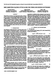
B. Directional Antenna Setup A motorized plat directional antenna assembly is fabricated to provide additional navigation accuracy at the close range. The antenna is mounted in front of the robot. A Kondo digital servo controls the antenna to scan a specific area or points to a particular angle. The maximum scan range of the servo is 270 degrees and the resolution is 270/4096 degree/step. The RSSI reading from the directional antenna is strongest if the radio source is in the middle of the antenna’s field of view. The readings fall off as the target move to the side of the field view. The further away the radio source is to the robot, the better angular resolution we can get. If the radio source is too close to the robot, the direction becomes indistinguishable due to RF signal saturation. At close range, the directional antenna is effective with the radio source placed one foot from the robot. The figure below shows the measured RSS of a source node three feet away from the robot. C. Outdoor experimental results Our outdoor experiment is conducted on VSU football field. Three Beacon nodes are deployed at the end of the field. To evaluate the performance of the navigation algorithm, we place a test wireless sensor node in the field as the target. The navigation algorithm will stop if it believes itself within

locations along the middle of the field. The results show that the navigation error is closely related to the relative distance between the target sensor and the beacon nodes. The starting location of the robot has little effect on the final result. The location error is less than 5 feet as long as the target sensor is within 120 feet from the beacon.

rssi m easure wit h direct ional ant enna 50 20e loc 1 20e loc 2 22e loc 3

45

rssi

40

35

30

25

VI. CONCLUSIONS 20

15 0

2

4

6

8

10

12

14

16

18

angle offset

Fig. 7. RSS vs Angular offset measured by Directional antenna in room HM22E, target-robot distance: 3 feet.

1 foot from the target. The actual distance to the target is measured manually as the location error. The measurement points are located from the goal line up to the 110-yd line every 10 yards; the total length of the field is about 330 feet. On each measured yard line, 5 data points are selected from sideline to sideline, making a grid size of 30 x 50 feet. The test area is about 160 feet in length. This is determined by a minimum RSS reading of 5. Although the Beacon packets can still be received after 110 yard line, there are many noticeable packet drops and moving robot further line will not generate any location estimation. Figure 8 (top)

35 30 25

100 90 80 70 60 50 40 30 20 10

20 15 10

x offset

5 0 120

100

80

60

40

20

y offset

0

0

navigat ion error in cent eral field 7

6

error (ft ))

5

4

3

2

1 0

20

40

60

80

100

120

140

160

180

200

dist ance (ft ))

Fig. 8.

(top) Outdoor RF profile, (bottom) location error

shows the 2-D RF profile we collected in the testing field from one of the beacon node. The bottom subfigure shows the navigation error when we place the test node at different

We present a radio sensing based location and navigation method for outdoor WSN applications. The method utilizes a vector of RSS measurements to estimate the location of the target sensor and optimum navigation direction. Our result shows that RSS based navigation can achieve reasonable accuracy in a coarsely profiled field. R EFERENCES [1] O. Hach, R. Lenain, B. Thuilot, P. Martinet, Avoiding steering actuator saturation in off-road mobile robot path tracking via predictive velocity control, IROS11, San Francisco, USA, september 26th - 29th, 2011. [2] Sebastian Thrun, Dieter Fox, Wolfram Burgard, Frank Dellaert, 2001, Robust Monte Carlo localization for mobile robots, Artificial Intelligence: 128, [3] Nando de Freitas, et al., “Diagnosis by a Waiter and a Mars Explorer”, Proc Of The IEEE, Special Issue on Sequential State Estimation, April 2003. [4] P. Bahl and V. Padmanabhan. Radar: An in-building rf-based user location and tracking system. In INFOCOMM, 2000. [5] David Moore, John Leonard, Daniela Rus, and Seth Teller. Robust distributed network localization with noisy range measurements. In Proceedings of ACM Sensys-04, Nov 2004. [6] Kamin Whitehouse, Chris Karlof, and David Culler, A practical evaluation of radio signal strength for ranging-based localization, SIGMOBILE Mob. Comput. Commun. Rev. 11, 1 (January 2007), 41-52. [7] Sangjin Han , Sungjin Lee , Sanghoon Lee , Jongjun Park , Sangjoon Park, Node distribution-based localization for large-scale wireless sensor networks, Wireless Networks, v.16 n.5, p.1389-1406, July 2010 [8] T. Oka, M. Inaba and H. Inoue, 1997, Describing a Modular Motion System based on a Real Time Process Network Model, in Proceedings of the 1997 IEEE/RSJ International Conference on Intelligent Robots and Systems. [9] J. Bachrach and C. Taylor, 2005, Localization in Sensor Networks, in Handbook of Sensor Networks: Algorithms and Architectures. [10] Cesare Alippi, Giovanni Vanini, Wireless Sensor Networks and Radio Localization: a Metrological Analysis of the MICA2 received signal strength indicator, 29th Annual IEEE International Conference on Local Computer Networks (LCN’04). [11] Edwin Olson, Johannes Strom, Rob Goeddel, Ryan Morton, Pradeep Ranganathan, and Andrew Richardson, Exploration and mapping with autonomous robot teams, ACM Commun, 56, 3 (March 2013), 62-70. [12] S. Lanzisera, D.T. Lin, and K.S.J. Pister. Rf time of ight ranging for wireless sensor network localization. pages 1-12, June 2006. [13] David Culler, Deborah Estrin, and Mani Srivastava. Guest editors introduction: Overview of sensor networks. Computer, 37(8):41-49, 2004. [14] F. Gustafsson et al., ”Particle filters for positioning, navigation, and tracking,” IEEE Transactions on Signal Processing, 2002. [15] Tong Liu, Paramvir Bahl, Imrich Chlamtac, Mobility Modeling, Location Tracking, and Trajectory Prediction in Wireless ATM Networks, IEEE Journal on Selected Areas in Communications, vol. 16, no. 6, 1998 [16] David S. Touretzky and Ethan J. Tira-Thompson. 2005. Tekkotsu: a framework for AIBO cognitive robotics. In Proceedings of the 20th national conference on Artificial intelligence - Volume 4 (AAAI’05), Anthony Cohn (Ed.), Vol. 4. AAAI Press 1741-1742. [17] Jayesh H. Kotecha, et al., “Gaussian Particle Filtering”, IEEE Trans on Signal Processing, Vol.51, No.10, 2003, pp 2592 - 2601.