COMMUNICATION PROTOCOLS FOR WIRELESS COGNITIVE RADIO AD-HOC NETWORKS
A Dissertation Presented to The Academic Faculty by Kaushik R. Chowdhury
In Partial Fulfillment of the Requirements for the Degree Doctor of Philosophy in the School of Electrical and Computer Engineering
Georgia Institute of Technology August 2009
COMMUNICATION PROTOCOLS FOR WIRELESS COGNITIVE RADIO AD-HOC NETWORKS
Approved by: Professor Ian F. Akyildiz, Advisor School of Electrical and Computer Engineering Georgia Institute of Technology
Professor Douglas Blough School of Electrical and Computer Engineering Georgia Institute of Technology
Professor Mary Ann Ingram School of Electrical and Computer Engineering Georgia Institute of Technology
Professor Konstantinos Dovrolis College of Computing Georgia Institute of Technology
Professor Ye Li School of Electrical and Computer Engineering Georgia Institute of Technology
Date Approved: 5 June 2009
To my family, for always being there at the end of the day.
iii
ACKNOWLEDGEMENTS
I would like to thank my advisor Professor Ian Akyildiz for giving me the opportunity to work under him, and for his thoughtful guidance during the entire Ph.D program. I am grateful to him for the trust he placed in me when I was rather untested, for his encouragement towards seeking an academic position, and for instilling an unwavering belief in my own modest abilities. I shall remember not only the research discussions, but also the many little lessons in life explained through his own personal experiences. I wish to express my gratitude to all the academic members of the Electrical and Computer Engineering Department at the Georgia Institute of Technology for their excellent advice, constructive criticism, helpful and critical reviews throughout the Ph.D. program. A special thank goes to Drs. Mary Ann Ingram, Ye Li, Douglas Blough, and Constantine Dovrolis, who kindly agreed to serve in my Ph.D. Defense Committee. I am thankful to all the members of the Broadband Wireless Networking Laboratory, both past and present, for the help received during my research, and also for the support that brought us together as a family. I would specifically like to mention the valuable contribution of Drs. Marco DiFelice and Tommaso Melodia, who have served in various capacities as my collaborators, friends and mentors over the past several years. Last but not least, the author is grateful to the many anonymous reviewers that with their comments greatly improved the content of the papers from which this thesis has been partly extracted.
iv
TABLE OF CONTENTS DEDICATION . . . . . . . . . . . . . . . . . . . . . . . . . . . . . . . . . . .
iii
ACKNOWLEDGEMENTS . . . . . . . . . . . . . . . . . . . . . . . . . . . .
iv
LIST OF FIGURES . . . . . . . . . . . . . . . . . . . . . . . . . . . . . . . .
viii
SUMMARY . . . . . . . . . . . . . . . . . . . . . . . . . . . . . . . . . . . . .
xi
I
INTRODUCTION . . . . . . . . . . . . . . . . . . . . . . . . . . . . . .
1
1.1 The Cognitive Radio Ad-hoc Network Architecture . . . . . . . . .
5
1.2 Research Objectives and Solutions . . . . . . . . . . . . . . . . . .
6
1.2.1
TP-CRAHN: A Transport Protocol for Cognitive Radio Adhoc Networks . . . . . . . . . . . . . . . . . . . . . . . . . .
7
SEARCH: A Routing Protocol for Mobile Cognitive Radio Ad-hoc Networks . . . . . . . . . . . . . . . . . . . . . . . .
8
1.2.3
Common Control Channel Design for Cognitive Radio Networks
9
1.2.4
Link Layer Spectrum Sensing and Sharing Framework for Wireless Mesh Networks . . . . . . . . . . . . . . . . . . . .
1.2.2
1.2.5
Interferer Detection, Channel Selection and Transmission Adaptation for Wireless Sensor Networks . . . . . . . . . . . . . 10
1.3 Organization of the Thesis . . . . . . . . . . . . . . . . . . . . . . . II
III
10
11
TP-CRAHN: A TRANSPORT PROTOCOL FOR COGNITIVE RADIO AD-HOC NETWORKS . . . . . . . . . . . . . . . . . . . . . . . . . . . 13 2.1 Motivation and Related Work . . . . . . . . . . . . . . . . . . . . .
14
2.2 Protocol Description . . . . . . . . . . . . . . . . . . . . . . . . . .
17
2.3 Performance Evaluation . . . . . . . . . . . . . . . . . . . . . . . .
24
2.3.1
Spectrum Sensing . . . . . . . . . . . . . . . . . . . . . . .
25
2.3.2
Spectrum Change and PU Activity . . . . . . . . . . . . . .
27
2.3.3
Mobility Prediction . . . . . . . . . . . . . . . . . . . . . . .
28
SEARCH: A ROUTING PROTOCOL FOR MOBILE COGNITIVE RADIO AD-HOC NETWORKS . . . . . . . . . . . . . . . . . . . . . . . . 30 3.1 Motivation and Related Work . . . . . . . . . . . . . . . . . . . . . v
30
3.2 Protocol Description . . . . . . . . . . . . . . . . . . . . . . . . . .
IV
3.2.1
Route Setup: . . . . . . . . . . . . . . . . . . . . . . . . . .
37
3.2.2
Route Enhancement . . . . . . . . . . . . . . . . . . . . . .
46
3.3 Route Maintenance . . . . . . . . . . . . . . . . . . . . . . . . . . .
48
3.4 Analysis of the Protocol . . . . . . . . . . . . . . . . . . . . . . . .
52
3.5 Performance Evaluation . . . . . . . . . . . . . . . . . . . . . . . .
54
COMMON CONTROL CHANNEL DESIGN FOR COGNITIVE RADIO NETWORKS . . . . . . . . . . . . . . . . . . . . . . . . . . . . . . . . . 62 4.1 Motivation and Related Work . . . . . . . . . . . . . . . . . . . . .
65
4.2 CCC Subcarrier Allocation . . . . . . . . . . . . . . . . . . . . . .
67
4.2.1
V
36
OFDM based Subcarrier Optimization Framework . . . . .
68
4.3 CCC Operation . . . . . . . . . . . . . . . . . . . . . . . . . . . . .
72
4.3.1
Broadcast Messaging . . . . . . . . . . . . . . . . . . . . . .
72
4.3.2
Unicast Messaging . . . . . . . . . . . . . . . . . . . . . . .
73
4.4 Performance Evaluation . . . . . . . . . . . . . . . . . . . . . . . .
79
4.4.1
Broadcast Messaging . . . . . . . . . . . . . . . . . . . . . .
81
4.4.2
Unicast Messaging . . . . . . . . . . . . . . . . . . . . . . .
85
LINK LAYER SPECTRUM-SENSING AND SHARING FRAMEWORK FOR WIRELESS MESH NETWORKS . . . . . . . . . . . . . . . . . . 89 5.1 Motivation and Related Work . . . . . . . . . . . . . . . . . . . . .
91
5.2 Preliminaries . . . . . . . . . . . . . . . . . . . . . . . . . . . . . .
92
5.2.1
System Operation . . . . . . . . . . . . . . . . . . . . . . .
93
5.3 Spectrum Sensing . . . . . . . . . . . . . . . . . . . . . . . . . . . .
95
5.3.1
Use of the Backoff Interval for Channel Sensing . . . . . . .
95
5.3.2
Centralized Framework for Time-domain Sensing . . . . . .
96
5.4 Distributed Approach to Sensing . . . . . . . . . . . . . . . . . . . 100 5.5 Analytical Interference Model . . . . . . . . . . . . . . . . . . . . . 102 5.6 Spectrum Sharing Framework . . . . . . . . . . . . . . . . . . . . . 106 5.7 Discussion of the Framework . . . . . . . . . . . . . . . . . . . . . 108
vi
5.8 Performance Evaluation . . . . . . . . . . . . . . . . . . . . . . . . 109 VI
INTERFERER DETECTION, CHANNEL SELECTION AND TRANSMISSION ADAPTATION FOR WIRELESS SENSOR NETWORKS . . 118 6.1 Motivation and Related Work . . . . . . . . . . . . . . . . . . . . . 119 6.2 Interferer Identification using Spectrum Signature . . . . . . . . . . 120 6.2.1
WLAN and Microwave Oven Experiments . . . . . . . . . . 120
6.2.2
Channel Selection . . . . . . . . . . . . . . . . . . . . . . . 125
6.3 Interferer-aware Transmission Adaptation (ITA) . . . . . . . . . . . 125 6.4 Performance Evaluation . . . . . . . . . . . . . . . . . . . . . . . . 128 VII CONCLUSION . . . . . . . . . . . . . . . . . . . . . . . . . . . . . . . . 132 REFERENCES . . . . . . . . . . . . . . . . . . . . . . . . . . . . . . . . . . . 135
vii
LIST OF FIGURES 1
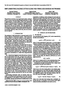
The cognitive radio cycle. . . . . . . . . . . . . . . . . . . . . . . . .
2
2
The cognitive radio ad-hoc network architecture. . . . . . . . . . . . .
5
3
The inability of the TCP cwnd to match the available bandwidth (a) and finite state machine model of our proposed transport protocol (b).
16
The effect of sensing time on detection error probability (a) and the scaling of the cwnd (b). . . . . . . . . . . . . . . . . . . . . . . . . . .
21
The effect of spectrum sensing on the throughput is shown for 1 and 5 flows in (a) and (b), respectively. Variation of the congestion window with time is given in (c). . . . . . . . . . . . . . . . . . . . . . . . . .
24
The effect of dynamically changing the sensing duration on throughput is shown for 1 and 5 flows in (a) and (b), respectively. . . . . . . . . .
25
7
A study of the throughput as a function of the varying sensing time. .
26
8
The effect of the bandwidth scaling adjustment on throughput is shown for 1, and 5 flows in (a), and (b), respectively. . . . . . . . . . . . . .
27
9
The bandwidth utilization efficiency. . . . . . . . . . . . . . . . . . .
27
10
The Kalman filter accuracy and the variation in the cwnd with time are shown in (a) and (b), respectively . . . . . . . . . . . . . . . . . .
29
11
Different coverage regions in different channels.
. . . . . . . . . . . .
31
12
Using greedy geographic forwarding on a given channel. . . . . . . . .
36
13
The PU avoidance phase with the focus region . . . . . . . . . . . . .
39
14
The joint path and channel decisions at destination. . . . . . . . . . .
42
15
Route maintenance with PU awareness. . . . . . . . . . . . . . . . . .
49
16
Circumventing the PU region and the associated path detour. . . . .
52
17
The effect of packet size on the end-to-end latency and the packet delivery ratio are shown in (a) and (b) respectively. . . . . . . . . . .
56
4 5
6
18
The packet delivery ratio, the end-to-end latency, and the number of hops for the case of 5 channels are shown in (a), (b), and (c) respectively, 56
19
The end-to-end latency and the packet delivery ratio are shown in (a) and (b) respectively for different PU ON times. A snapshot of the latency is plotted against the simulation time in (c). . . . . . . . . . .
viii
58
20
The packet delivery ratio, the end-to-end latency, and the number of hops for the case of 10 channels are shown in (a), (b) and (c) respectively. 59
21
CCC operation using guard bands in the licensed spectrum. . . . . .
63
22
The relationship between the transmission symbol and its frequency domain sinc function. . . . . . . . . . . . . . . . . . . . . . . . . . . .
68
23
The arms formed by the choice of guard bands. . . . . . . . . . . . .
75
24
The spectral interference overlap for 6 and 12 MHz licensed channels are given in (a) and (b), respectively. . . . . . . . . . . . . . . . . .
80
The interference caused to the PUs (a), the spectrum utilization efficiency (b), and throughput during CCC broadcast (c) are shown, respectively. . . . . . . . . . . . . . . . . . . . . . . . . . . . . . . . .
82
The spectral interference caused by activating the different number of subcarriers. . . . . . . . . . . . . . . . . . . . . . . . . . . . . . . . .
83
The number of times an arm is selected (spectrum opportunity) for 2 and 6 occupied PU channels are given in (a) and (b), respectively. . .
85
The number of distinct arms are plotted against the earned reward for 2 and 6 occupied PU channels in (a) and (b), respectively . . . . . . .
86
The number of available transmission opportunities for a given cumulative subcarrier bandwidth are given for 2 and 6 occupied PU channels in (a) and (b), respectively. . . . . . . . . . . . . . . . . . . . . . . .
87
The number of channels that can be sensed in a single duration for which the timer is frozen, for varying packet sizes and transmission rates is shown in (a). When received power is measured at channel 772 MHz, the combined effect of two primary stations 1 and 2 is the same as the single transmitter 3 (b). . . . . . . . . . . . . . . . . . .
94
The radio may switch to the primary channel for the duration of the packet transfer during the freeze duration, if it is not the intended recipient. . . . . . . . . . . . . . . . . . . . . . . . . . . . . . . . . . .
95
MC x! senses the channel when three primary stations are in the neighborhood. The received power is the sum of the individual transmit powers scaled by the spectral overlap factor. . . . . . . . . . . . . . .
97
25
26 27 28 29
30
31
32
33
Each hop reduces the number of variables by 1 and forwards it to the next hop. The return path is initiated at the M th node, and each time, all the solved values of the variables obtained are sent to the previous hop. This continues till all the unknowns are solved and finally communicated to the MR. . . . . . . . . . . . . . . . . . . . . 100
ix
34
Calculation of received power at user located at A due to a cluster of N nodes under MR B. . . . . . . . . . . . . . . . . . . . . . . . . . . 102
35
Effect of noise power on the accuracy of the analytically predicted frequencies used by the primary stations, for a constant number of sets (a) and the improvement in accuracy of prediction of the channels used by the primary stations with increasing number of sets (b). Graph (c) shows the relationship between the number of minimum required sensing nodes, for a given number of required sets and primary stations.110
36
The time overhead for the centralized (a) and distributed (c) schemes is compared . The time taken at each hop of the chain propagation for the distributed approach is shown in (b). . . . . . . . . . . . . . . . . 111
37
The analytical model is verified for increasing distance (a) and transmit power (b). . . . . . . . . . . . . . . . . . . . . . . . . . . . . . . . . . 112
38
The received power in each of the 16 channels of the primary band for the primary and secondary transmitters in shown in (a). The received power at each of the 11 channels of the secondary band at the central location is shown before (b) and after (c) the shift of the clusters 2, 3 and 6, into the primary band. . . . . . . . . . . . . . . . . . . . . . . 115
39
The topology considered for investigating the gains obtained through the band/channel shifting scheme. . . . . . . . . . . . . . . . . . . . . 116
40
The experimental setup to measure the WLAN and microwave interference (a) and the allowed conical region for classification of the interferer (b). . . . . . . . . . . . . . . . . . . . . . . . . . . . . . . . . . . . . . 121
41
The RSS for the WLAN (a), the microwave oven (b). . . . . . . . . . 122
42
The PSR for the WLAN (a), the microwave oven (b). . . . . . . . . . 122
43
The sensor transmits whenever the channel is free based on the WLAN traffic or microwave duty cycle. . . . . . . . . . . . . . . . . . . . . . 126
44
The probabilities for false alarm (FA) and missed detection (MD) for the spectral signature matching technique are given in (a) and (b), respectively. . . . . . . . . . . . . . . . . . . . . . . . . . . . . . . . . 128
45
The effect on the WLAN throughput (a), the energy consumption of the WSN in presence of WLAN (b) and microwave oven (c). . . . . . 129
x
SUMMARY
Cognitive radio (CR) technology allows devices to share the wireless spectrum with other users that have a license for operation in these spectrum bands. This area of research promises to solve the problem of spectrum scarcity in the unlicensed bands, and improve the inefficient spectrum utilization in the bands reserved for the licensed users. However, the opportunistic use of the available spectrum by the CR users must not affect the licensed users. This raises several concerns regarding spectrum sensing, sharing and reliable end-to-end communication in CR networks. This thesis is concerned with the design and implementation of communication protocols for the multi-hop infrastructure-less CR ad-hoc networks (CRAHNs). In addition, it also addresses the critical issue of interference-free spectrum usage in specific ad-hoc architectures, such as, resource-constrained wireless sensor networks and wireless mesh networks that have high traffic volumes. The problems of spectrum management that are unique to CR networks are first identified in this thesis. These issues are then addressed at each layer of the network protocol stack while considering the distributed operation in CRAHNs. At the physical layer an algorithmic suite is proposed that allows the CR devices to detect and adapt to the presence of wireless LANs and commercial microwave ovens. A common control channel is designed that allows sharing of the spectrum information between the CR users, even when the available spectrum varies dynamically. A spectrum sharing scheme for mesh networks is proposed at the link layer that allows cooperative detection of the licensed users and fair utilization of the available spectrum among the mesh devices. The spectrum availability and route formation are then considered jointly at the network layer, so that the licensed users are protected as well as the CRAHN performance is maximized. Finally, we extend the classical TCP at the transport layer to ensure end-to-end reliability in a multi-hop CR environment. xi
CHAPTER I
INTRODUCTION
The unlicensed spectrum bands in the 2.4 GHz range are being increasingly used by wireless mesh networks (WMNs), Wi-fi hotspots, wireless sensor networks (WSNs) and mobile ad-hoc networks for a variety of military, environmental monitoring and commercial applications. This has led to the problem of spectrum scarcity in the unlicensed band, which is also affected by the interfering radiation caused by commercial microwave ovens and electrical machinery. At the same time, the frequencies reserved for licensed use, such as television broadcast, are not always occupied, leading to inefficient utilization of the resource. The newly emerging cognitive radio (CR) paradigm is geared to addressing these issues by allowing the CR users to opportunistically transmit in the vacant portions of the licensed spectrum [7][55]. These radios may decide transmission parameters such as channel, power, modulation type, and transmission rate through local coordination based on their perception of the state of the network and the physical environment. The Federal Communications Commission (FCC) has encouraged work in spectrum sharing issues by initiating steps to free up bandwidth in the 54 − 72 MHz, 76 − 88 MHz, 174 − 216 MHz, and 470 − 806 MHz bands [29]. We consider the more general scenario in which the entire frequency ranges are not completely vacated, but may experience occasional transmissions by licensed users. We refer to these bands as primary bands and the licensed operators in them as primary users (PUs) in the subsequent discussion. In this research, we explore ways in which the CR ad-hoc network users, equipped with tunable radios, may share the primary band. It is imperative that PUs in these bands have priority in communication, and their operation
1
Figure 1: The cognitive radio cycle. must not be hindered by spectrum sharing techniques. Thus, the key challenges that must be addressed include identifying which portions of the spectrum are free for use, sharing the available spectrum, and adapting the transmission of the CR users so that the interference caused to PUs is minimized. Specifically, in CR ad-hoc networks (CRAHNs), the distributed multi-hop architecture, the dynamic network topology changes caused by mobility, and the time- and location-varying spectrum availability are some of the key distinguishing factors [5] [6]. In order to adapt to dynamic spectrum environment, the CRAHN necessitates the spectrum-aware operations, which form a cognitive cycle [7]. As shown in Figure 1, the steps of the cognitive cycle consist of four spectrum management functions: spectrum sensing, spectrum decision, spectrum sharing, and spectrum mobility. To implement CRAHNs, each function needs to be incorporated into the classical layering protocols. The followings are the main features of spectrum management functions: • Spectrum Sensing: A CR user should monitor the available spectrum bands, capture their information, and then detect spectrum holes. Spectrum sensing is a basic functionality in CR networks, and hence closely related to other spectrum management functions as well as layering protocols to provide information
2
on spectrum availability. • Spectrum Decision: Once the available spectrums are identified, it is essential that the CR users select the best available band according to their QoS requirements. Especially in CRAHNs, spectrum decision involves in jointly undertaking spectrum selection and the route formation. • Spectrum Sharing: The transmissions of CR users should be coordinated by spectrum sharing functionality to prevent multiple users from colliding in overlapping portions of the spectrum. Spectrum sharing includes channel and power allocations to avoid interference caused to the primary network and an intelligent packet scheduling scheme enabled by a spectrum-aware link layer along with spectrum sensing. • Spectrum Mobility: If the specific portion of the spectrum in use is required by a PU, the communication must be switched to another vacant portion of the spectrum. This requires spectrum handoff and reliable end-to-end connection management schemes, such as protocols at the transport layer that closely coupled with the lower level spectrum sensing, neighbor discovery in a link layer, and routing protocols. The above spectrum management-related challenges necessitate novel design techniques spanning several layers of the protocol stack on a single device, in addition to the interaction between several nodes. The difference between the classical and CR based wireless ad-hoc networks, with respect to end-to-end reliable communication over multiple hops, can be illustrated with the following example. In the classical case, the transmitted packets may incur a long delay time before reaching the destination, owing to network congestion or a temporary route outage. However, for CRAHNs, a similar effect on the packet latency may be caused if an intermediate node on the route is engaged in spectrum sensing and hence is unable to forward 3
packets. Also, the sudden appearance of a PU may force the CR nodes in its vicinity to limit their transmission, leading to an increase in the delay. Thus, it is important to integrate the effect of the CR spectrum sensing, sharing and PU awareness in an end-to-end protocol design. Moreover, in classical ad-hoc networks, the existing work on multi-channel architectures does not consider higher priority users in the same spectrum. Thus, there is no necessity of local or even network-wide synchronization to ensure the detection of the PUs that have preferential access to the spectrum. In CRAHNs, however, if network-wide synchronization is possible, then at pre-decided intervals, the CR users cease their data transmissions and listen for PU activity on the primary channels [51] [52] [88]. However, this is difficult to achieve in a distributed environment, where the sensing undertaken by the users is generally asynchronous. Ad-hoc networks include specialized architectures, such as wireless mesh networks (WMNs) and wireless sensor networks (WSNs). Each of these network architectures, while retaining the distributed nature of operation, have special considerations. The WMN network protocols must be optimized for speed, and thus, fast spectrum sensing and switching techniques should be devised. In addition, the traffic load must be balanced between the primary and the unlicensed bands to avoid performance degradation to the users connected to mesh routers that form the network backbone. On the other hand, the sensor nodes that compose the WSN are severely constrained in energy and computational power. Thus, the CR based protocols for WSNs must be light-weight, and have have the primary objective of reducing interference-related packet losses. The ultimate goal of this research is to address the end-to-end protocol design aspects for mobile CR ad-hoc networks, and also to provide spectrum sensing, sharing and transmission scheduling solutions specially adapted for the WMNs and WSNs. We believe that dynamic spectrum sharing may soon become a key technology for addressing the spectrum scarcity problem as new, untapped spectrum bands are
4
Mobile CR Ad−hoc Network TV Spectrum Band Fixed PU transmitter
MC
Gateway CR Wireless Mesh Network (WMN)
Fixed PU receiver MR Clusters
Public Service Band
Wireless Sensor Network (WSN)
Base Station
Mobile PU Transmitter/Receiver
Primary User Network Architectures
CR Ad−hoc Network Architectures
Figure 2: The cognitive radio ad-hoc network architecture. being identified. This thesis attempts to enable the seamless coexistence of the infrastructure-less CRAHNs and the PUs, resulting in better network performance, efficient resource utilization and meeting the application specified quality of service constraints. We begin by first describing the network architecture considered in our research, and the main contributions of the work.
1.1
The Cognitive Radio Ad-hoc Network Architecture
In CRAHNs, the CR users must learn about the state of the network and physical environment through local coordination with other users. This coordination becomes a challenge when the available spectrum varies with time, and the node mobility causes frequent route disruptions. In this section, the CR ad-hoc network architecture is described and the problems, resulting from the distributed operation, in each of the protocol stack layers are explained. As shown in Figure 2, the primary and the CR ad-hoc network coexist in the primary bands. The primary network is composed of primary users (PUs) that may be stationary or mobile. Television broadcast stations and receiver sets form the static topology PU network, while devices in the public service band may be mobile. For CR users, different ad-hoc architectures are possible and each of these may entail
5
a specialized protocol development. CR users can communicate with each other in a multi-hop manner on both licensed and unlicensed spectrum bands with the help of a single transceiver. The focus of this research is on mobile ad-hoc network architectures that do not have centralized infrastructure support and must coordinate among themselves for network operation. Ad-hoc networks also include specialized architectures, such as wireless mesh networks (WMNs) and wireless sensor networks (WSNs). A typical WMN consists of mesh routers (MRs) forming the backbone of the network, interconnected in an ad-hoc fashion. Each MR can be considered an access point serving a number of possibly mobile users or mesh clients (MCs) [9]. The MCs direct their traffic to their respective MRs, which then forward it over the backbone, in a multi-hop manner, to reach the gateway that links to the Internet. Wireless sensor networks (WSN) are composed of simple, resource-constrained nodes reporting to a base station and are being increasingly used for military, environmental monitoring, and data-gathering applications [8]. This research proposes protocol solutions so that these different CR ad-hoc architectures seamlessly coexist in the primary bands with the PUs. We mainly focus on the physical, link, network, and transport layers of the protocol stack to enable this and there exist several challenges in the implementation of the protocols.
1.2
Research Objectives and Solutions
In the following, we briefly describe these layer-specific challenges elaborated in the rest of the proposal. We follow a top-down approach, beginning with the transport layer and going over the network, link, and physical layers, in turn.
6
1.2.1
TP-CRAHN: A Transport Protocol for Cognitive Radio Ad-hoc Networks
The transport layer plays an end-to-end role in multi-hop CR ad-hoc networks. It provides reliable packet delivery and prevents congestion along the chosen route.Existing research in transport protocols for wireless ad-hoc networks has focused on reliable end-to-end packet delivery under uncertain channel conditions, route failures due to node mobility and link congestion. In a cognitive radio (CR) environment, there are several key challenges that must be addressed apart from the above concerns. The intermittent spectrum sensing undertaken by the CR users, the activity of the licensed users of the spectrum, large-scale bandwidth variation based on spectrum availability, and the channel switching process need to be considered in the transport protocol design. As the transport protocol usually runs at the end nodes (source and destination), it has limited knowledge of the conditions of the intermediate nodes. Unknown to the source, the route may be disconnected due to node mobility. Also, packet losses may be wrongly attributed to network congestion rather than bad channel conditions at the link layer. Classical TCP suffers from some of the above issues and efforts have been made to address them for wireless scenarios in [50][77]. However, these protocols for classical wireless ad-hoc networks do not consider the spectrum-related issues that may arise in CR ad-hoc networks. In this research, a window-based TCP-like Transport Protocol for CR Ad-Hoc Networks, TP-CRAHN, is proposed that distinguishes each of these events by a combination of explicit feedback from the intermediate nodes and the destination [24]. TCP, in general, is a well researched area and several theoretical models exist that explain and predict its behavior in wireless networks [83]. Our work adapts the classical TCP rate control algorithm running at the source to closely interact with the physical layer channel information, the link layer functions of spectrum sensing and
7
buffer management, and a predictive mobility framework that is developed at the network layer. 1.2.2
SEARCH: A Routing Protocol for Mobile Cognitive Radio Ad-hoc Networks
The CR users in a distributed network may not be within direct transmission range of each other, and intermediate nodes must forward packets between them. The first step in this is setting up optimal routes over multiple hops to the destination at the network layer. In CRAHNs, this is undertaken by joint spectrum selection and the route formation. Efficiently leveraging this node level channel information in order to provide timely end-to-end delivery over the network is a key concern for CR based routing protocols. To enable this, there exist several centralized solutions [60][10][82][43][84] that require extensive network information or specialized data structures that cannot be disseminated easily through the multi-hop ad hoc network. The existing distributed networks solve the routing problem sequentially, often optimizing the route first and then performing spectrum allocation [19], which may not always yield a feasible solution. The PUs affect the licensed channels to varying extents, depending on the proportion of the transmission power that gets leaked into the adjacent channels. This also affects the geographical region, in which the channel is rendered unusable for the CR users. In this research, a geographic forwarding based SpEctrum Aware Routing protocol for Cognitive ad-Hoc networks (SEARCH), is proposed that (i) jointly undertakes path and channel selection to avoid regions of PU activity during route formation, (ii) adapts to the newly discovered and lost spectrum opportunity during route operation, and (iii) considers various cases of node mobility in a distributed environment by predictive Kalman filtering [23]. Specifically, the optimal paths found by geographic forwarding on each channel are combined at the destination with an aim to minimize the hop count. By binding the route to regions found free of PU
8
activity, rather than particular CR users, the effect of the PU activity is mitigated. 1.2.3
Common Control Channel Design for Cognitive Radio Networks
The available spectrum resource changes dynamically with the PU activity, necessitating frequent PU sensing coordination, exchanging network topology information, and adapting the functioning of the end-to-end higher layer protocols in a multi-hop CRAHN. In such cases, the coordination must occur over a common control channel (CCC) that is not interrupted by the changing PU activity, thereby ensuring a continuous active connection between the CR devices. The existing approaches are mainly concerned with forming clusters [16][17][87] of CR users or allowing them to establish pair-wise connections over frequency hopping sequences [26][42]. The above approaches may suffer from disruption when the channel used for the CCC is reclaimed by the PUs. Thus, an always-on, out-of-band design is proposed in this research that uses non-contiguous OFDM subcarriers placed within the guard bands separating the channels of the licensed spectrum. First, the task of choosing the OFDM specific parameters, including the number, power, and bandwidth of the subcarriers is formulated as an optimization problem to ensure that the CCC meets the CR user demands, and at the same time, does not adversely affect the PU operation. Secondly, the probability of an overlap in the power spectrum close to the guard band-PU channel boundaries is further minimized by appropriate selection of the active subcarriers in a distributed manner by the CR users. To enable this, the multi-arm bandit algorithm is used that allows the guard bands (and hence, the subcarrier choices) to evolve over time, thus reflecting the state of the PU induced interference.
9
1.2.4
Link Layer Spectrum Sensing and Sharing Framework for Wireless Mesh Networks
The function of the link layer is primarily to coordinate the access to the wireless channel. Apart from this, in a CR ad-hoc network, it must also prevent the transmission of CR users in the primary band from affecting the communication of the PUs. Thus, the spectrum-sensing and sharing functions must also be performed by the link layer. In a WMN, as there are several mesh clients (MCs) in each cluster, the sensing information can be collected from more than one MC. Devising a framework where this sensed data is collected from the mesh clients and combined to improve the accuracy is an important issue. Additionally, the WMNs experience a high volume of traffic, necessitating smaller durations of dedicated channel-sensing time. With these considerations, we propose a cooperative and distributed spectrumsensing and network load-aware spectrum sharing technique for WMNs [21]. The approach in this research is along the lines of [31] and [68] but without the limitations posed by the number of users and the presence of auxiliary sensing devices, respectively. 1.2.5
Interferer Detection, Channel Selection and Transmission Adaptation for Wireless Sensor Networks
At the link layer, it is important to identify the interferer type and its specific operational characteristics and accordingly adapt the scheduling functionality. This effort is supported by the physical layer, in which the channel characteristics and transmission spectrum are studied for obtaining information about the PUs. For sensor networks, the recent work has mainly focussed on measuring the performance degradation caused by the effect of WLAN and microwave technologies on the devices based on the IEEE 802.15.4 standard [64][69][71][85]. In this research, we develop an interferer identification technique for WSNs that
10
allows the sensor nodes to classify the interferers in the ISM band into WLAN devices and commercial microwave ovens [22]. This is done by comparing the observed spectral shape with the known spectral signature for these devices obtained by prior experimentation. Moreover, this allows the sensor nodes to adapt their transmission schedules based on the interferer type. Our proposed method solves the problem of interference-related packet losses in the WSN, a key reason for packet losses in the resource-constrained nodes.
1.3
Organization of the Thesis
This thesis is organized as follows. In Chapter 2, we propose a window-based Transport Protocol for CR Ad-Hoc Networks called TP-CRAHN that distinguishes the spectrum-related events and adapts to them by altering the transmission rate at the source appropriately. In Chapter 3, we present the SEARCH routing protocol that jointly undertakes route formation and spectrum assignment. The route setup and management stages are discussed in detail. In Chapter 4, we propose a CCC framework that uses OFDM subcarriers spread over the guard bands separating the licensed channels. Our CCC design approaches for both the Broadcast and Unicast messaging functions are provided. In Chapter 5, we describe a spectrum sensing and sharing framework for CR WMNs, called COMNET that allows the distributed mesh clients to sense the licensed channel occupancy through cooperative sensing, and also allows the spectrum resource to be shared fairly among the mesh clusters. In Chapter 6, we present our experimental results on the interference caused by WLAN and commercial microwave oven based on our sensor testbed. We also design algorithms that allows the sensors to detect a particular type of the interferer and alter their packet scheduling at the link layer accordingly.
11
Finally, in Chapter 7, we draw the main conclusions and outline future research directions.
12
CHAPTER II
TP-CRAHN: A TRANSPORT PROTOCOL FOR COGNITIVE RADIO AD-HOC NETWORKS
The mobility of the intermediate nodes and the inherent uncertainty in the wireless channel state are the key factors that affect the reliable end-to-end delivery of data in classical ad-hoc networks. However, several additional challenges exist in a CR environment. The periodic spectrum sensing, channel switching operations, and the awareness of the activity of the primary users (PUs) are some of the features that must be integrated into the protocol design. In this research, we propose a windowbased, TCP-like spectrum-aware transport layer protocol for CR ad-hoc networks, called TP-CRAHN, that distinguishes between these different conditions in order to undertake state-dependent recovery actions [24]. Transport protocols for classical wireless ad-hoc networks do not consider the cases that may arise in CR ad-hoc networks. As an example, in a classical wireless ad-hoc network, packets may incur a longer round trip time (RTT) owing to network congestion or due to a temporary route outage. In CR ad-hoc networks, a similar effect on the packet RTT may be caused if an intermediate node on the route is engaged in spectrum-sensing and hence, unable to forward packets. Also, the sudden appearance of a primary user may force the CR nodes in its vicinity to limit their transmission, leading to an increase in the RTT. In such cases, the network is partitioned until a new channel is identified and coordinated with the nodes on the path. The duration of the periodic spectrum-sensing decides, in part, the end-to-end performance - a shorter sensing time may result in higher throughput but may affect the transport layer severely if a PU is mis-detected. While several works have
13
focussed on spectrum-sensing algorithms in the last few years [7], the integration of the channel information collected at the nodes and the performance study of these approaches from the viewpoint of an end-to-end protocol remains an open challenge. In this research, we investigate how the CR functionalities may be integrated at the transport layer for reliable and congestion-free packet delivery.
2.1
Motivation and Related Work
Our transport protocol addresses the following concerns in CR ad-hoc networks: • Spectrum Sensing: CR users periodically monitor the current channel over a pre-decided sensing duration for the occurrence of PUs before using it for transmission. During this interval, the nodes are not actively involved in transmitting data packets and the multi-hop network is virtually disconnected at the node that is engaged in spectrum-sensing. This may result in acknowledgement (ACK) packets not arriving timely at the source, or a buffer overflow at the node just prior to the node undertaking sensing. Moreover, choosing the appropriate sensing duration for the intermediate nodes has a significant impact on the end-to-end performance [72], as the network remains disconnected during these events. This duration cannot be assumed to be the same for all the nodes of the path, as regions experience different levels of PU activity. • PU Activity: On detecting the presence of a PU, the CR users cease their operation on the affected channel and search for a different vacant portion of the spectrum. While the spectrum-sensing on the current channel is periodic and has a well-defined interval, the time taken to coordinate with the next hop neighbors for determining a mutually acceptable channel is of an uncertain duration. Thus, the source may need to be paused for an indefinite time till a new channel is negotiated.
14
The spectrum sensing time and the delay induced by PU arrivals also influence the way in which notifications about route failures should be used in the CR ad-hoc transport protocols. In classical ad-hoc networks, ATCP [50] and TCP-EFLN [35] react to the route disruption after it happens by an explicit notification in the form of the Internet Control Message Protocol (ICMP) message at the IP layer. A classical scheme for for reducing the packet losses by routing layer feedback is proposed in [86]. However, this method uses cached routes and does not involve new route discovery. For CRAHNs, the changing spectrum environment may not guarantee the feasibility of the cached route. Thus, we believe that a predictive framework is needed so that source can restrict its sending rate in advance of the route failure and limit the number of transmitted packets, when the notification of failure is actually received. • Spectrum Change: A key concern in CR networks is the efficient utilization of the spectrum resource, as the opportunity for transmission in the licensed bands is available for a limited time. The licensed channels may have a large variation in bandwidth, especially as nodes switch from one spectrum band to the other. In Figure 3(a), we show the latency in the TCP congestion window (cwnd ) when the available bandwidth of the channel dynamically changes values from the set { 31 Mbps, 43 Mbps, 2 Mbps}. We observe that the cwnd has a slow variation compared to the available spectrum bandwidth (shown by the vertical lines), leading to inefficient use of the spectrum. Estimating the new operating point for the transmission window size at the source is a challenge, as increasing the cwnd rapidly may usher in a sudden congestion situation, while a low value may not utilize the resource completely. Bandwidth estimation techniques have been proposed in [14][53] that do not require information from the intermediate nodes, but also do not respond immediately to the available spectrum.
15
(a) Mobility Predicted
Connection ACK/ Est. Timeout
Network Layer Information
Synchronized ACK/ Timeout
Periodic Sensing
ICMP ECN/ ACK
ECN/ ACK
Spectrum Sensing
Normal
PU Detect. EPN PU Detect. EPN
Route Failure
CHN
Spectrum Change
ICMP ICMP
ACK/ Timeout
(b)
Figure 3: The inability of the TCP cwnd to match the available bandwidth (a) and finite state machine model of our proposed transport protocol (b).
16
2.2
Protocol Description
Our design extends the classical TCP and the preliminary finite state machine of the protocol is shown in Figure 3(b) [24]. It involves the following six states: (i) Connection Establishment, (ii) Normal, (iii) Spectrum Sensing, (iv) Spectrum Change, (v) Mobility Predicted, and (vi) Route Failure. The descriptions of these states and their transitions are described next. A. Connection Establishment: TP-CRAHN modifies the three-way handshake in TCP newReno so that the source can obtain the sensing schedules of the nodes in the routing path. First, the source sends out a synchronization (SYN) packet to the destination. An intermediate node, say i, in the routing path appends the following information to the SYN packet: (i) its ID, (ii) a timestamp, and (iii) the tuple {t1i , t2i , tsi }. Here, t1i is the time left before the node starts the next round of spectrum sensing, measured from the timestamp. t2i is the constant duration between two successive spectrum sensing events, and tsi is the time taken to complete the sensing in the current cycle. On receiving the SYN packet, the receiver sends a SYN-ACK message to the source. The sensing information collected for each node is piggybacked over the SYN-ACK and thus, the source knows when a node in the path shall undertake spectrum sensing and its duration. The final ACK is then sent by the source to the destination completing the handshake. We note that the calculation of the sensing time tsi by a node i is undertaken locally. Based on the bandwidth of the channel (W ), the external signal to noise ratio (γ), and the probabilities of the on period (Pon ) and the off period (Pof f ), a framework to calculate this time is given as follows [47], tsi =
Pof f Pf 2 1 [Q−1 (Pf ) + (γ + 1)Q−1 ( )] . 2 W ·γ Pon
(1)
Equation (1) gives the sensing time tsi that minimizes the probability of missed primary user detection Pf , i.e., incorrectly stating the channel is vacant when indeed 17
there is an active PU and Q is the standard Q function. The sensing times collected from the nodes are the preliminary values which are dynamically updated by TPCRAHN. State Transitions: On successful handshake, the source and destination are synchronized and the Normal state is entered. B. Normal State: This state is similar to the classical TCP newReno where the congestion window, cwnd, is increased based on the incoming ACKs. The congestion is notified to the source through the explicit congestion notification (ECN) message. Here, our protocol evaluates if the ECN is still relevant to the network congestion state by checking if the time lag from its generation at the affected node to its reception is within the time lag threshold Lmax . If no prior action has been taken for an earlier ECN from the same node, for the detected congestion event, TP-CRAHN reduces the cwnd to 1 and cuts the ssthresh by half. The measured link latency and bandwidth at the intermediate nodes are also piggybacked over the ACK. As the complete path is connected in this state, an average end-to-end round trip time (RTT) is also maintained at the source. The intermediate nodes of the path piggyback the following link-layer information over the data packets to the destination, which is then sent back to the source through the ACK. Residual buffer space (Bif ): Consider a node i that has Biu bytes currently of unoccupied buffer space. Let the number of flows passing through it be nfi . The fair share of the residual buffer space per flow is, Bif =
Biu nfi
.
Observed link bandwidth (Wi,i+1 ): Each node i maintains a weighted average of the observed bandwidth on the link formed with its next hop, i.e. {i, i + 1}, during the normal state. This is obtained from the link layer as the ratio of the acknowledged data bits to the time taken for this transfer between the nodes i and i + 1. Total link latency (LTi,i+1 ): Let Li,i+1 be the sum of the (i) time taken by a packet
18
of the current flow to move to the head of the queue (ii) the time for contending the access to the channel and finally, (iii) the transmission time measured at node i with respect to the next hop i + 1. The total link latency is now defined considering the bidirectional link latencies, LTi,i+1 = Li,i+1 + Li+1,i . Apart from these fields that are updated every time by the nodes, the ACK also carries the ECN notification whenever a node experiences congestion and the mobility predicted flag (MF), when a possible route outage is identified. State Transitions: The ECN message and the ACKs regulate the cwnd. When a node in the path performs sensing, TP-CRAHN transitions into the Spectrum Sensing state. If PU activity is reported to the source through an Explicit Pause Notification (EPN), it enters the Spectrum Change state and resumes the usual operation on receiving the information about the new channel through the Channel (CHN) message. Possible route disruptions may be signaled by the information contained in the ACKs, leading to the temporary Mobility Predicted state, where the cwnd is restricted to ssthesh. If the ICMP message is received, TP-CRAHN enters into the Route Failure state and stops transmission. C. Spectrum Sensing State: During intermittent sensing by a node i in the path, say, the TCP connection suffers from temporary disconnection. At this time, our protocol ensures that node i − 1 previous to node i does not suffer from a buffer overflow. This is achieved by considering the minimum of the buffer space remaining f at the previous hop node Bi−1 , the current congestion window cwnd and the receive f window advertised by the destination. This residual buffer space Bi−1 is periodically
decreased based on the last estimate of the link latency obtained from the incoming ACKs. For the nodes that are present in regions with very little spectrum outages, the sensing time is reduced. Also, this reduction is more when the sensing time is large, and progressively smaller values are used as the sensing time itself is decreased. This
19
follows from the non-linear relationship between the optimal sensing time needed to detect the PU under a given missed-detection error probability [48] and is shown in Figure 4(a). We observe that the ts is large when the target error probability is very low. Moreover, there is also a large fall in the ts for a finite change in the Pf , when the Pf is small. This means that the ts can be reduced by a greater margin in the initial stage, when it has a comparatively higher duration, without impacting the error significantly. Also this margin must itself be lowered as the value of ts gets progressively reduced. The intuitive reasoning is as follows: A node i first sets ts = tsmax corresponding to the low error probability of Pf = 0.1. If the number of spectrum changes that occur over time, is small in proportion to the number of total changes along the entire path, we assume that the node is situated in a region with limited PU activity. Thus, the periodic sensing time tsi may be reduced at this node. If the current tsi at the node is large, its reduction is consequently higher, as the probability of error is not affected proportionally. However, as the tsi value falls, the reduction gets progressively smaller until tsi = tsmin is reached, corresponding to the limiting error probability, Pf = 0.5. We can now formulate the steps for obtaining the new sensing duration tsi (new) from the old value tsi as follows, tsmax 2 dts γtsi = |ts =tsi , Pf =f unc(tsi ) dPf dts |ts =tsmax , Pf =0.1 γtsmax = dPf γts δis = − i · "t γtsmax "t =
tsi (new) = tsi − δis .
(2) (3) (4) (5) (6)
The default decrement value of the sensing time, "t , is taken as half of the maximum value, tsmax , needed to maintain the error probability at 0.1, as shown in (2). This is later scaled by a factor in the range [0, 1] to get the true decrement δis . In (3), 20
0.9
B’
SNR =−20dB SNR =−22.5dB SNR =−25dB
0.8
0.6
cwnd
Sensing time (s)
0.7
0.5 0.4
B
ssthresh
0.3 0.2 0.1 0 0.1
0.15
0.2
0.25 0.3 0.35 Missed Detection Probability
0.4
0.45
(a)
0.5
time (b)
Figure 4: The effect of sensing time on detection error probability (a) and the scaling of the cwnd (b). we calculate the value of the gradient γtsi to the sensing curve at the current sensing duration tsi , at node i. The corresponding value of Pf is obtained from the current tsi from Figure 4(a), which is in turn, a numerical plot of equation (1). The maximum gradient of the sensing curve γtsmax is given in (4) and is computed at tsi = tsmax . The normalized gradient,
γts i
γtsmax
, at the current tuple given by {tsi , Pf } is used as the scaling
factor to give the true decrement δis in (5). Finally, the sensing time is adjusted to the new value tsi (new) in (6). When successive missed detection events occur, the node increases the sensing duration in the steps { 12 · tsmax ,
3 4
· tsmax , tsmax }, in that order. Whenever the sensing
time is changed, the node sends back the new value to the sources of the flows passing through it by piggybacking over the ACK. In order to identify a specific node i for adjusting the sensing time, TP-CRAHN ranks the nodes in the path based on the number of times the operational channel was changed due to PU activity. It keeps a count of the CHN messages sent by each node of the path, which reveals the number of times the connection was paused while a new-channel was being coordinated. Intuitively, the node that generated the highest proportion of the CHN message also experienced the maximum number of PU detection events and thus, must be located in a region of frequent PU activity.
21
Such a node needs to retain a higher sensing duration. D. Spectrum Change State: When the spectrum at a link changes, because of a PU arrival, an explicit pause notification (EPN) is sent to the source and our protocol enters the Spectrum Change state. After choosing the new spectrum and channel, the nodes on that link roughly estimate the new link latency and bandwidth. This information is then sent to the source through the channel (CHN) message. On receiving the new estimated bandwidth, the source checks to see if this is the new bottleneck bandwidth on the path and if this value is significantly different from the previous bottleneck. If this is so, the cwnd is scaled, say, from the current value marked by B to a new value given by B ! in Figure 4(b). This scaling is based on the new estimated bottleneck bandwidth and the RTT, so that so that it can adjust its sending rate to immediately reflect the new channel conditions. We consider the case where TP-CRAHN adjusts to a single affected link {i − 1, i}. The set of available channels is known at node i. The preferred list of channels, from this available set, is sent by this node to the previous hop i − 1. The node i − 1 chooses a channel from this set, say ξqx . It then sends back a link layer ACK to node i to inform the node of its choice, ξqx . All the coordination up to this point occurs on the old channel. A second set of Probe and ACK messages are then exchanged on the channel to be switched, ξqx , as a confirmation and also to approximately estimate the new link transmission delay times Li,i−1 and Li−1,i . If the probe and ACK packets are of the size Pprobe and PACK , respectively, the observed link bandwidth Wi,i−1 is, Wi,i−1 =
Pprobe + PACK . Li,i−1 + Li−1,i
(7)
The CHN message contains in it the bidirectional link layer packet delay over the newly identified channel, (LTi,i−1 = Li,i−1 +Li−1,i ) that is used by the source to calculate Wi,i−1 from equation (7). We recall that the ACKs forwarded over the intermediate hops also carry the total bidirectional link latency, L! Ti,i−1 , corresponding to the earlier used channel. On receiving the CHN message, the source first estimates the new RTT 22
using (i) the earlier observed RTT’ during the last normal state of the protocol and (ii) adjusting for the new bidirectional link delay, LTi,i−1 , as RT T = RT T ! +LTi,i−1 −L! Ti,i−1 . For the given path of n nodes, let Wb! be the old observed bottleneck bandwidth, before the channel change. After the channel change, the new bottleneck bandwidth is identified as Wb , where Wb = min{Wl,l+1}, l = 1, . . . , n − 1. The updated estimate of the bandwidth Wi,i−1 is used in this calculation from equation (7). If the ratio of the old bottleneck bandwidth to the new is within the allowed range of [1 − $, 1 + $], i.e.,
Wb! Wb
∈ [1 − $, 1 + $], then no scaling of the earlier cwnd is needed, where $ = 0.2.
If it lies beyond this range, then we calculate the new value of the cwnd as follows, cwnd = αc · Wb · RT T.
(8)
The factor αc = 0.8 in equation (8) is used to adjust the cwnd to a value slightly lower than the predicted bandwidth to prevent the risk of over-estimating the cwnd. State Transitions: The Spectrum Change state is entered as soon as an EPN message is received. It reverts back to the Normal state when the new channel information is received in the CHN message or enters into the Route Failure state on the receipt of an ICMP message. Existing sensing schedules are ignored as long as the protocol stays in the current state. E. Mobility Predicted State: The periodic sensing and the occasional spectrum changes undertaken by the nodes on the path may cause the route failure message may arrive late at the source. Our protocol incorporates a Kalman filter based prediction [39] of an impending route failure that proactively limits the sending rate of the source. This limiting condition on the cwnd may be canceled if no route failure actually occurs within a specified timeout period. F. Route Failure State: This is the terminal state of the current cycle and a fresh TCP connection must be established when a new route is formed. The protocol enters this state on receiving the route failure message (ICMP) and the source must cease transmission immediately. The key challenge in this state is identifying that a 23
(b)
(a)
(c)
Figure 5: The effect of spectrum sensing on the throughput is shown for 1 and 5 flows in (a) and (b), respectively. Variation of the congestion window with time is given in (c). node has indeed moved out of range as opposed to (i) a sudden loss of communication because of PU arrival, and (ii) bad channel conditions, leading to bursty packet losses is an issue that needs to be addressed. To enable this, close coupling with the allowed number of link layer packet retries and the mobility prediction mechanism described above may be needed.
2.3
Performance Evaluation
In this section, we study the behavior of TP-CRAHN under the scenarios of (i) spectrum sensing, (ii) spectrum change with PU activity, and (iii) node mobility. Rather, we use TCP newReno (henceforth referred to as TCP) as a benchmark and
24
(a)
(b)
Figure 6: The effect of dynamically changing the sensing duration on throughput is shown for 1 and 5 flows in (a) and (b), respectively. focus on how TP-CRAHN adjusts to each of the above CR scenarios through a stagewise implementation of its modules. We extend the NS-2 simulator with multi-channel extensions and a channel switching time of 5 ms is used. In order to study the effect of the cwnd scaling, we consider 5 channels, C = {c1 , . . . , c5 }, having varying raw channel B B bandwidth given by {B, K , B · K, K , B · K}, respectively, where B = 2 Mbps, K = 2.
In addition, a priority queue is implemented at the link layer, and the allowed retries for the feedback packets in TP-CRAHN is raised to 20. Out of 100 nodes any sourcedestination pair is chosen forming a chain topology and we vary the number of flows in the path. The transmission ranges of the PU and the CR users are 300 m and 120 m, respectively and the desired throughput τd = 800 Kbps. 2.3.1
Spectrum Sensing
The evaluation of TP-CRAHN during spectrum sensing is carried out in two parts - (i) by observing the improvement in throughput resulting from the change in the ewnd, and (ii) the benefit of reduction of the sensing duration in the absence of PU activity. Figures 5(a) and 5(b) show the end-to-end throughput for varying network loads as the sensing time of the nodes is increased to the maximum value ts = tsmax = 0.3,
25
Figure 7: A study of the throughput as a function of the varying sensing time. for a constant data transmission time Tp . In the first set of experiments, we disable the dynamic adjustment of the sensing time. We observe that TP-CRAHN outperforms TCP significantly as it does not stop transmitting when the path gets disconnected, but transmits at a reduced rate to prevent a buffer overflow. This ensures a higher throughput in TP-CRAHN, as TCP suffers an RTO timeout whenever a node in the path undertakes sensing. This phenomenon is also seen in Figure 5(c), where the cwnd almost never reduces to 1 for the case ts = 0.15, Tp = 3, unless there is congestion in the network (at sim. time = 70 s). Compared to this, TCP undergoes repeated timeouts during the sensing and the cwnd is forced to the slow start phase in the absence of true congestion. For the study of the dynamically changing sensing duration, we first define the PU operation as follows: We continuously vary the on time (Ton ) of the PU on the x-axis, and measure the throughput for different PU off times, Tof f , for 1 and 5 flows as shown in Figures 6(a) and 6(b), respectively. We first assign a low PU susceptibility of 0.01 to a randomly chosen number of nodes Slow in the path, and for the remaining nodes, forming the set Shigh , we set an initial high susceptibility value of 0.95. This ensures that TP-CRAHN changes the sensing duration from the maximum value tsmax = 0.28 only for the nodes present in the set Slow . When the sensing time is dynamically by TP-CRAHN, (shown by sensing time 26
(a)
(b)
Figure 8: The effect of the bandwidth scaling adjustment on throughput is shown for 1, and 5 flows in (a), and (b), respectively. Bandwidth Utilization Efficiency (%)
0.5
TCP TP−CRAHN
0.4 0.3 0.2 0.1 0
1
2 3 4 5 Bandwidth Difference Factor (K)
6
Figure 9: The bandwidth utilization efficiency. = var), we observe that the throughput improves significantly for both the cases of 1 and 5 flows (Figure 6(a) and 6(b)). The variation of the cwnd for throughput as a function of the changing sensing time is shown in Figure 7.The sensing time falls in a non-linear manner, and improves the throughput in the absence of PU activity. For successive PU missed detections, the sensing time is scaled to 21 ·tsmax , then 43 ·tsmax and finally to the maximum value tsmax . For each increase in ts , though the throughput is partially reduced, the mutual interference with the PU is also mitigated. 2.3.2
Spectrum Change and PU Activity
When PU activity is detected, TP-CRAHN stops the source from transmitting and coordinates the use of a new channel. The source then modifies its cwnd, if the new 27
channel on the affected link significantly changes the bottleneck bandwidth available to the connection. We study the performance improvement in TP-CRAHN by considering the throughput, the bandwidth efficiency (ratio of the available bandwidth to average used bandwidth of the bottleneck link), and the variation in the cwnd. A PU is placed on each of the 5 possible channels so that the channel (and hence, the bandwidth) change often and its effect is clearly demonstrated. Figures 8(a) and 8(b) give the throughput for 1 and 5 flows, respectively, when PUs exist on the channel. We observe that the throughput improvement in TP-CRAHN increases with higher PU activity, formally defined as σ =
Ton . Ton +T of f
For lower values of σ, i.e.,
when Ton is small, the channels are readily available and the gain in TP-CRAHN is due to the scaling of the cwnd alone. For higher values of σ, when Ton is large, it takes longer for the affected node to find a vacant channel. This delay dominates the network performance and by explicitly specifying the source to pause its transmission, TP-CRAHN prevents packet loss and improves the throughput. The effect of cwnd scaling results in higher bandwidth efficiency in TP-CRAHN, as seen in Figure 9. Moreover, the performance improves when the difference in the raw bandwidths of the available channels (given by increasing the factor K) is higher, implying that the forced scaling of the cwnd is effective in fully utilizing the spectrum resource. 2.3.3
Mobility Prediction
The error between the true signal strength (RSS) and the value predicted by the Kalman filter is shown in Figure 10(a) as a function of the epoch interval used between two successive calculations. In our chain topology, nodes move with an average speed of 10 m/s with locations given by the random waypoint model. The variance (var) in the RSS in dB, due to external noise affects the prediction accuracy as shown in the figure. We observe two cases in Figure 10(b), the first of which shows a route
28
(a)
(b)
Figure 10: The Kalman filter accuracy and the variation in the cwnd with time are shown in (a) and (b), respectively disconnection at time = 70 s. The conservative reduction in the cwnd resulted in fewer packets that were lost in the unusable route, as compared to TCP. An incorrect prediction that restricted the cwnd to the ssthresh till the timeout period is shown at time= 150 s.
29
CHAPTER III
SEARCH: A ROUTING PROTOCOL FOR MOBILE COGNITIVE RADIO AD-HOC NETWORKS
Efficiently leveraging node level channel information in order to provide timely endto-end delivery over the network is a key concern for CR based routing protocols. In addition, the primary users (PUs) of the licensed band affect the channels to varying extents, depending on the proportion of the transmission power that gets leaked into the adjacent channels. This also effects the geographical region, in which the channel is rendered unusable for the CR users. In this research, a geographic forwarding based SpEctrum Aware Routing protocol for Cognitive ad-Hoc networks (SEARCH), is proposed that (i) jointly undertakes path and channel selection to avoid regions of PU activity during route formation, (ii) adapts to the newly discovered and lost spectrum opportunity during route operation, and (iii) considers various cases of node mobility in a distributed environment by predictive Kalman filtering [23]. Specifically, the optimal paths found by geographic forwarding on each channel are combined at the destination with an aim to minimize the hop count. By binding the route to regions found free of PU activity, rather than particular CR users, the effect of the PU activity is mitigated.
3.1
Motivation and Related Work
• Awareness of Primary User Activity: Existing routing protocols for ad-hoc networks do not account for the region affected by an active PU and are unaware of the changing spectrum opportunity. In CR networks, routes must be constructed to avoid these regions and must also adapt themselves to subsequent
30
z Frequency (MHz)
R4
Ch 4
R5
5 MHz
Ch 5
R6
5 MHz
Ch 6
5 MHz
R7 Ch 7
5 MHz
R8 Ch 8
O l S1
x
y
1
l S2
WLAN 2
Figure 11: Different coverage regions in different channels.
changes induced by new PU arrivals. We discuss this further for geographic routing protocols, as the route formation in SEARCH is based on this principle. Geographic routing protocols for classical wireless networks rely on a greedy positive advance towards the destination [38]. By knowing the location of the destination and that of the candidate forwarding nodes within its range, a node can choose the next hop that gives the greatest advance. Whenever a void is encountered, the path traverses the perimeter of the void and then resumes the greedy forwarding to the destination. However, in a CR network, as the PUs have precedence in accessing the spectrum resource, the routing protocol must compromise on the greedy advance when it intersects a region of PU activity. Two possible solutions to this are: circumventing the affected region or switching the affected channel. The choice between these options needs to made
31
taking into account the overall end-to-end performance. Classical geographic routing protocols are oblivious to these PU specific considerations and limit their operation to a single channel. SEARCH, on the other hand, provides a hybrid solution. It first uses greedy geographic routing on each channel to reach the destination by identifying and circumventing the PU activity regions. The path information from different channels is then combined at the destination in a series of optimization steps to decide on the optimal end-to-end route in a computationally efficient way. • Global Channel Switching vs Path Detour Decisions: From practical considerations, the channels are not completely orthogonal and a finite amount of transmitted power leaks into the adjacent channels. This constitutes the spectral leakage power, which is a source of the interference in the affected channels. Based on the proportion of the leakage power, channels used by the CR may be affected to different geographical extents due to a single PU. As an example, consider Figure 11, in which a WLAN transmitter is located at the origin O and follows the IEEE 802.11b standard [3]. The x − y axes represent the two dimensional cartesian space and the z axis is the frequency scale. S1 and S2 are two other nodes that sense the transmitted power and are at a distance of (1 and (2 , respectively, from the WLAN where (1 > (2 . The nodes S1 , S2 and the WLAN lie in the x − y plane. When the WLAN transmits on channel 6, the nodes observe the leakage power by tuning to the channels Ch : 4, 5, 7 and 8, each separated by a difference of 5 MHz. The spectral shape of the WLAN signal is such that the leakage power is high in the frequencies close to that of the transmission channel, and falls as one moves further away on the frequency scale. This radius of coverage is shown by R4 , . . . , R8 for the WLAN channels Ch : 4, . . . , 8, respectively. We observe that node S1 is further away from the origin, as compared to S2 , and is within the coverage radius of the WLAN on 32
channel 6 only. Node S2 , being closer to the WLAN, is under the coverage range of all the channels considered above. Extending this example for CR networks, a single PU located at the origin may affect the channels used by the CR users, say S1 and S2 , differently. As the extent of the coverage is not completely known at a given node, a local channel switching decision may not be optimal in a network-wide context. From Figure 11, consider a path that passes through the nodes S1 and S2 . Node S1 finds itself under the PU coverage region on channel 6 and switches to a free channel, say 5. The subsequent route, however, intersects the PU coverage region in the new channel within a few hops, when node S2 is reached. In addition, the node S1 does not have any information about the extent of the detour that will be required if the route formation is continued on the affected channel 6. SEARCH solves this problem by estimating the route detours on each channel, taking into account their dissimilar coverage ranges. It then computes whether the cost of the detour is less than the added delay in switching the channel, with respect to the end-to-end latency. • Cognitive Radio Specific Mobility Concerns: The node mobility is one of the chief factors of route outages in ad-hoc networks. Specifically, in a CR environment, we identify a new problem arising out of mobility that needs to be addressed. Consider the case in which the nodes continue to form a connected route but may stray, due to their mobility, in the coverage region of a PU on the current channel. Thus, even though the route is connected, the nodes in the PU region may be unable to transmit. We recall that SEARCH uses anchor locations for routing that are found to be free of PU activity. It addresses the CR mobility concerns by checking if the next hop node is within a threshold distance of the anchors. If this condition is not satisfied, the forwarding node identifies a new next hop that is closest to the anchor, thus ensuring that PU 33
regions are always avoided. The centralized framework presented in [60] defines a link disruption probability to simulate PU activity. It is assumed that this probability is known before network operation through some estimation techniques. The routing problem is formulated as an optimization goal that minimizes the total average delay, which is determined by: (i) the volume of data that must be sent, (ii) the mean capacity of the path as a function of the spectrum and link disruption probabilities, and (iii) channel propagation delay. Another centralized approach [10] addresses flow fairness in which the complete knowledge of the flows between any two nodes is known. Here, a network-wide optimization problem is solved and a constant factor approximation to the optimal solution is provided. A graph theoretic approach is given in [82], wherein non-overlapping channels and time slots over a two hop range are assigned through the creation of independent sets if the entire network graph is known. Two routing algorithms that require the network topology at each node are provided in [43] for optimizing the path latency and number of channel switches, respectively. In [84], a layered graph is constructed which has the available channels in vertical layers, and the classical network graph showing the node adjacencies along each layer. The nodes within communication range on a given channel (layer) have a horizontal edge between them. All the channels that are usable at a given node are connected by a vertical edge. The cost of an edge traversal is appropriately set depending on the time cost of switching a channel (vertical edge) as opposed to the forwarding of the packet on the same channel (horizontal edge). However, in mobile networks, collecting the entire network topology is infeasible. This approach serves as the optimal centralized solution for routing algorithms with static topologies. Distributed approaches scale well in an ad-hoc network and require comparatively less computation at the end destination. However, a key problem faced in the design of distributed routing protocols is that the path and channel decisions are made 34
sequentially and not together. The best routing paths are first identified and then the preferred channels along the path are chosen in [19]. Here, the ad-hoc distance vector (AODV) routing protocol is modified to include the list of preferred channels by a given node as the route request (RREQ) is forwarded through the channel. Once the RREQ is received, the destination is aware of the channels that may be used to transmit at each hop and finds the optimal combination such that channel switching is minimized. The route formation in the SEARCH protocol is based, in part, on geographic routing. This principle is used in GPSR that undertakes greedy forwarding under normal conditions and enters into perimeter mode when a void (region with an absence of forwarding nodes) is encountered [38]. In order to circumvent this void, it requires the construction of a planar graph of the network at each node at all times or the creation of network-wide spanning trees [49]. However, this constitutes an overhead as only a few selected nodes need to participate in the perimeter forwarding mode. the classical GPSR has also been modified for particular application scenarios, such as, mobile vehicular networks in GPCR [27] and GPSRJ++ [46]. However, they need street level knowledge of roads and junctions, thus restricting their application. Mobility considerations are addressed in [20, 73] based on local single-hop information. Through periodic beacon exchanges, a node signals if it is in a dead-end region and prevents itself from being chosen as the next hop during greedy forwarding in [20]. By estimating the velocity based on location updates through beacon messages, a node can estimate when the next hop will go out of range in [73]. However, this neither provides a solution to a large scale destination mobility, nor re-evaluates the optimality conditions of the current path periodically. SEARCH is a completely distributed routing solution that accounts for PU activity, mobility of the CR users and jointly explores the path and channel choices
35
A
x
lx
θ max Source S θ max
ly
y
Dest. D
lz
RT
z B
Figure 12: Using greedy geographic forwarding on a given channel.
towards minimizing the path latency. It reflects on the true channel delay by conducting the route exploration in the actual channels used for data transfer. We now list the assumptions regarding the network architecture in the next section.
3.2
Protocol Description
SEARCH attempts find the length of the shortest path based on greedy advancement that may be traversed on a combination of channels to the destination. The key functionality in our proposed approach is evaluating when the coverage region of the PU should be circumvented, and when changing the channel is a preferred option. First, the shortest paths to the destination, based on geographic forwarding and consideration of the PU activity, are identified on each channel. The destination then combines these paths by choosing the channel switching locations, with an aim to minimize the number of hops to the destination. In this section we shall describe the initial protocols functions in two parts: (i) the route setup phase and the (ii) route enhancement that is undertaken to improve the route, once it is in operation.
36
3.2.1
Route Setup:
In this stage, a route request (RREQ) is transmitted by the source on each channel that is not affected by the PU activity at its current location. It gets forwarded by intermediate hops till it reaches the destination, with each intermediate node adding in the packet its (i) ID, (ii) current location, (iii) time stamp and (iii) a flag status indicating the current propagation mode of the algorithm. SEARCH operates in two modes - Greedy Forwarding and PU Avoidance, depending on whether the RREQ is propagating along the greedy shortest path to the destination or needs to circumvent a region of PU activity, respectively. Finally, the routes on the individual channels are combined at the destination by the Joint Channel-Path Optimization algorithm. Greedy Forwarding Through the exchange of beacon messages, each CR user is aware of the locations of the other nodes within its transmission range. Thus, knowing the location of the destination, a protocol based on greedy geographic forwarding can decide which of the candidate forwarders of the RREQ should be chosen as the next hop to minimize the distance to the destination. While SEARCH shares the principle of geographic forwarding with other related ad-hoc protocols like [38], the next hop is not always chosen purely on the greedy advance metric in our approach. The two distinguishing features are: • The RREQ forwarding process must occur on the same channel and the chosen next hop must not be under a PU coverage region on the current transmission channel. As an example, from Figure 11, node S2 cannot participate in the route formation on the channels 4, . . . , 8. It may, however, forward the arriving RREQs on the other channels that are not affected by the PU transmission. • The chosen forwarder must lie in a specific region around the current hop, called as the focus region, which we define later in this section. Thus, a node with
37
a lesser advance towards the destination but within the focus region is chosen over another node closer to the destination that lies outside this area. In Figure 12, the source S has the nodes x, y and z within its transmission radius RT . These nodes are at a straight line distance of lx , ly and lz , respectively, from the destination D, where lx > ly > lz . The focus region for S is shown by the sector S − AB and extends to an angle of θmax from the line SD. Classical geographic routing protocols like GPSR would have chosen node z at this stage, while SEARCH chooses the node with the greatest advance within its focus region, i.e., node y. If no such node exists, then SEARCH switches from the greedy forwarding phase to the PU avoidance phase. We now define the focus region formally with reference to Figure 12, Definition 1 Focus Region: Consider a straight line path, SD from a given node S to the destination D. The sector with transmission radius RT , centered at the location of the node S and extending up to a maximum angular spread of θmax on either side of SD, gives the focus region for this node.
Definition 2 Decision Point: A node that lies in the focus region of the previous hop along the path, but does not find a forwarding node for the RREQ in its own focus region, is called the decision point.
The focus region is shown as the shaded area in Figure 12. If the nodes x and y do not participate in the routing process, then node S would not have any candidate forwarder within its focus region. It would mark itself as a decision point, as per Definition 2. Knowing the decision point (DP) gives an intuitive idea of the locations of the PUs and the occupied channels. We recall that the nodes within the coverage region of a 38
Resume Greedy Forwarding
c
b
b
RT
c θ max
d A a
x
d
θ max a
x
θ max
(DP) θ max
Dest. D
Dest. D
(DP)
Enter PU Avoidance
RT
B
(a)
(b)
Figure 13: The PU avoidance phase with the focus region
PU do not take part in the RREQ forwarding process. Thus, they are virtually absent from the network topology on the affected channels and do not feature in the focus region as candidate forwarder nodes. Not finding any feasible node, this previous hop now labels itself as the DP and enters into the PU avoidance stage. When the RREQ is received at the destination, it knows the point on the route, i.e., the DP location, from which the path enters into a detour to avoid the PU region. SEARCH then attempts to find out alternate paths (and hence channels) at these detour locations. While our approach may decrease the per-hop advancement, it allows SEARCH to identify a large deviation from the straight line path to the destination. We note that if a void (region where no nodes are present) is encountered, the same process is followed. Thus, unlike GPSR [38], SEARCH does not need to maintain the planar graph information when it encounters regions that need to be avoided. PU Avoidance When a PU region is encountered, rendering the channel in its vicinity unusable, the greedy forwarding towards the destination can no longer be carried out. This stage is called the PU avoidance stage as the RREQ now starts circumventing around the affected region. We explain this as follows: Figure 13(a) shows the shaded circular area under the influence of a PU on the
39
channel being used for forwarding the RREQ. In addition, the focus region for node x on this channel, from Definition 1, is given by the sector x − AB with the maximum angle of 2 · θmax . Some of the nodes that sense the PUs and do not participate in the forwarding of the RREQ, lie in the focus region of the node x. Through the periodic beacon update, these affected nodes inform their one-hop neighbors, including node x, of the current state of the channel environment. Thus, node x is aware that the closest node to the destination that can forward the RREQ (node a) lies outside its focus region. From Definition 2, node x concludes that it is a DP and sets the PU avoidance (PA) flag in the RREQ packet before re-transmitting it. The DP marks the point from which the route must circumvent the region of PU activity on the given channel. There may be several such DPs in the path to the destination and this information is collected by the RREQ as it traverses through the network. The PA flag in the RREQ remains set till a node is reached that has a candidate forwarder in its focus region. In the example shown in Figure 13(b), the RREQ traverses the node a, b and finally reaches node c. The latter has a candidate forwarder, node d that lies in its focus region. At this point, i.e., at node d, the PA flag is reset, signaling the end of the avoidance phase and the greedy forwarding is resumed. Joint Channel-Path Optimization If the licensed band is completely free of PU activity, then there are no regions that must be avoided in any of the channels. Thus, the RREQs sent on the different channels would chart similar paths to the destination. In the presence of PUs, however, some nodes do not participate in the route setup stage if they are in the affected region on these channels. Consequently, the paths traversed by the RREQs in the different channels are not the same. The optimization phase of the SEARCH protocol is designed to choose a combination of channels and the propagation paths along them that minimize the end-to-end latency. This optimization is performed at the destination based on the information contained in the received RREQs. We first
40
explain the underlying idea by the following example and then formally define the optimization algorithm. In Figure 14, each plane represents a channel and the broken line shows the path obtained by the propagation of the RREQ on each of them. This path is limited on one channel and is a combination of the greedy forwarding and PU avoidance phases. Though all the nodes are located in the same physical space, only a subset of them are shown that participate in the routing on a given channel, depending on their individual PU coverage regions. These nodes form the anchor points on their respective channels. Let the RREQ on channel 1 give the shortest path from the source to the destination D, among all the considered channels. A portion of this path from node x to D is shown. Let node x be the decision point (DP) where the path starts avoiding the PU affected region on channel 1. Our optimization framework tries to identify if a better channel (and hence, path) may be used at the DP, thereby preventing the additional hops incurred in channel 1. To allow a path switch at node x, the new path must have the node x in common, or must be within the transmission range of x. Thus, only the paths in channels 2 and 3 are considered as the nodes y and z are within range of x on these channels, respectively. The path on channel 4, being at a distance of at least two hops from node x cannot be included in this stage. If the path on channel 1 is switched to a different channel, say channel 2, then the packet traverses on the path in channel 1 till node x and then on the path on channel 2 from node y to the destination. The channel, and hence, path change occurs at node x if the sum of the (i) path latency in the new channel from node y to the destination, (ii) the estimated time to reach node y from node x, and (iii) the cost of the switching the channel ts is less than the path delay from node x to the destination in channel 1. As the new path is traversed, the above conditions are checked for each new DP encountered in the route. If multiple channels exist that
41
Channel 1
x
(DP)
Dest. D Channel 2
x Dest. D
y
Channel 3 z x
Dest. D Channel 4 w
x
Dest. D Links for merging paths Original greedy paths
Figure 14: The joint path and channel decisions at destination.
provide a better path alternative, one of them is chosen that minimizes the total latency to the destination. From Figure 14, the time to destination may be smaller for channel 2 as compared to continuing on channel 1 or switching to channel 3, and thus, it is chosen at the node x. A brief analysis of these two options of route detour as opposed to channel switching is presented for an ideal case in Appendix A. We define the variables used in the subsequent discussion as follows: The RREQ received on a given channel, say k, defines a path of lk anchor points given by Pk = {A1k , A2k , . . . , Alkk }. The anchor points are the locations of the nodes that were chosen during the forwarding process of the RREQ packet and indicate the absence of PU activity. Some of these anchors may also serve as decision points (DP) depending on whether the path encounters a PU region. The optimal greedy path PG is a combination (or union) of anchor points and the channel switching decisions shown by Cjk,i, indicating that the channel is changed from k to i at the hop j. The transmission time for a packet on channel i is given as TRi and the total number of channels in the band is C. We can formally express the route selection at the destination through the following algorithm steps.
42
• Step 1. Initial Path Selection: The destination D receives the RREQs on each channel k ∈ C and extracts the path information Pk from it. The path Pk is compsed of a set of nodes {Ajk } with their respective timestamps {tjk }, where j = 1, . . . , lk and the final node is the destination, i.e., Alkk = D. We first define the latency, Lm k , from an intermediate point m to the final node lk on the lk channel k based on their respective timestamps, tm k and tk , as follows: lk m Lm k = tk − tk .
(9)
As the first optimization step, considering the propagation from the first node of the route (m = 1), the least latency path Lm k is chosen among all the available channels k ∈ C using equation (9), i = argk min{L1k , ∀k ∈ C}
(10)
In this step, the greedy path solution PG is initialized to the start node on the channel i as PG = A1i . This set will grow as the choice of nodes and channel switching decisions are added progressively in the subsequent steps of the algorithm. • Step 2. Greedy Path Formation: The least latency path may be further improved by switching to a different channel at the DPs. This is because the initial path having the minimum end-to-end delay, may not be continuously optimal through the intermediate path segments. In this step, SEARCH attempts to improve the chosen route by considering intersecting paths on the other channels that may be locally optimal. The DPs are chosen for this optimization as the path starts curving at these locations and better paths on different channels that follow a shorter route to the destination may exist. Formally the next hop
43
node, Aj=j+1 , along the current chosen path on channel i is added to PG , if it is i not a DP. This step is repeated in a loop as long as a DP is not reached. Thus, j =j+1 ! PG = PG Aji , if Aji %= DP.
(11)
If this next hop is the final destination, then the algorithm is terminated and the path is complete. In this case, SEARCH proceeds to Step 5 directly. If this is not so, and the next hop is indeed a DP, the local optimality condition is checked in Step 3. • Step 3. Optimization at the DP: When a DP is reached, SEARCH attempts to find an intersecting path on a different channel at this location. A given path P1 with node x is said to be intersecting with another path P2 , if the latter (i) has the node x common or (ii) has a node that is within transmission range of node x in path P1 . From Figure 14, the paths shown in channels 2 and 3 are intersecting with the path on channel 1 as the nodes y and z in these paths, respectively, are within transmission range of the node x. Given the channel switching time ts and the time to transmit a packet TRk on channel k, the time overhead, δk , to reach the node in the intersecting path is: δk = ts + TRk , k ∈ C.
(12)
The current channel i (and hence, the path) may be switched to an intersecting path (say, on channel k) at the node m in the transmission range of the DP j, only if the latter has a smaller latency to the destination measured from j. Also, the transmission range (RT ) constrains the allowed distance between the two j m nodes Aji and Am k by the inequality dist(Ai , Ak ) < RT . The total time taken to
reach the destination is given by Lm k + δk , if channel k is chosen. Also, if more than one intersecting path exists, the new channel k is so chosen that the time 44
to destination is minimized over all the possible channel options. Assuming the transmission range as RT , the tuple {hop number m! , channel k ! } is chosen that minimizes the total time Lm k + δk , {m! , k ! } = arg{m,k} min {Lm k + δk } dist(Aji , Am k ) < RT , ∀k ∈ C.
(13)
• Step 4. Route Expansion: The greedy path solution is updated with the new channel and path information. First, the channel switching decision shown !
by Cji,k , is incorporated in the final path PG , along with the node Am k ! that !
serves as the next hop in the new path.
PG = PG
!
Cji,k
!
!
!
Am k! .
(14)
Finally, the new channel k ! is now the default channel, i.e., i = k ! , j = m. The procedure of traversing the new path by checking the DPs is repeated from Step 2. • Step 5. Route Confirmation: When the last hop i.e., the destination is reached, the route reply RREP is sent back to the source along the optimal route PG . The RREP contains the IDs of the nodes, the anchor locations and the channel switching decisions. The routing of data packets can begin immediately when the source receives the RREP. During the route setup stage, the destination optimizes the path and channel choices based on nodes that are within transmission range of each other to give the optimal path PG . The next stage of optimization, route enhancement, occurs when the route is active and attempts to combine paths that are separated by more then one hop. 45
3.2.2
Route Enhancement
The route enhancement stage comes into operation after the initial route setup stage and conservatively explores the gains of linking together paths formed on different channels that are up to η hops away. From Figure 14, if the DP x is a part of the optimal route at the end of the route setup phase, this stage of the protocol may allow it to reach node w two hops away, on the least latency path in channel 4. The algorithm for enhancing the current route is as follows: • We recall that the route setup phase checks for a possible path (and channel) change at each DP. If there is no other node within the transmission range, the DP is retained in the current path. In this phase, the currently used shortest path PG is further optimized considering (i) all the remaining DPs on it, and (ii) the anchor points on the other routes (hence, on the other channels) that are within η hops of the considered DP. We assume that the currently used optimal path is composed of a set of anchor points given by PG = {A1G , . . . , AqG }. Formally, SEARCH chooses the DP on the optimal path (AiG ) and the anchor Am k on channel k that must be reached, to minimize the total distance to the destination. Here, the first constraint is that i i m the node Am k must be within η hops of the DP AG , i.e., dist(AG , Ak ) < η · RT .
The maximum allowed physical distance between the two nodes is given by the product of the hop count η and the transmission range, RT . On similar lines, the actual number of hops, ηi,m,k , between these two nodes is given by, ηi,m,k
dist(AiG , Am k ) < η where AiG = DP. = RT
(15)
If TRk is the transmission time for a packet on channel k ! for a single hop, the total estimated time taken to traverse this distance of ηi,m,k hops is ηi,m,k ·TRk . In order to find the tuple {i! , m! , k ! } that minimizes the total cost to the destination among all the possible combinations, we add the time to the destination from 46
the new next hop mLm k and the channel switching time ts . Additionally, this time has to be smaller than the path latency, LiG , from the considered DP to the destination if the routing is continued on the existing path. We formulate this optimization equation to find the tuple {i! , m! , k ! } as follows, " # i {i! , m! , k ! } = argi,m,k min (ηi,m,k · TRk + Lm k + ts ) < LG ∀AiG ∈ PG , and AiG = DP ∀k ∈ C, ∀Am k ∈ Pk , ηi,m,k < η.
(16)
Summarizing the above discussion and from equation (15), we explain the constraints as follows: A node AiG in the optimal path PG may be used in the minimization only if it is a DP. We consider the path Pk in each of the possible channels k in the channel set C. In these paths we allow the anchor points as a candidate solution if it is within η hops of the DP being considered. • Once a feasible path is identified by the destination, it sends a route enhance!
ment (ROP) message to the DP AiG , found in the earlier step. The ROP contains !
(i) the ID of the node Am k ! that must be reached on the new path, (ii) the path !
information in terms of successive next hop nodes from the intended node Am k!
to the destination. We recall that both of this information is obtained from the RREQ received on channel k ! during the route setup stage. !
!
• The DP AiG receiving the ROP now sends an RREQ message with the node Am k!
as the destination, similar to the route-setup phase involving greedy forwarding. The new path information received in the ROP is then included in the RREP when it is forwarded on the channel k ! . A key difference in the route enhance!
ment phase is that, on receiving the RREQ, node Am k ! continues to forward it 47
towards the eventual destination D. The RREQ may be dropped if either the !
target node Am k ! cannot be reached in η hops, or the route (indicated by the node IDs in the RREQ) is disconnected at any point before the destination is reached. • If the destination receives the forwarded RREQ, it checks if the actual latency on the new path is lower than the value on the current path from the DP !
AiG . If so, an RREP is sent along the new route and an RERR is propagated along the earlier route indicating the formation and the teardown of the routes, respectively. In this process, the portion of the optimal path PG after the DP !
AiG is deleted and the new path information is added. Thus, !
i +1 PG = PG /{AG , . . . , AD G} ! ! +1 PG = PG {Am , . . . , AD k ! }. k!
(17)
• This run-time optimization continues till all the DPs in the current optimal path PG , have been explored and no further improvement in latency is observed. We note that this optimization process does not affect the current route operation as it is carried out in parallel. However, this stage is implemented immediately after the route is operational as mobility of the nodes may change the path conditions found in the route setup phase for the other channels. We next describe the route management functions of the SEARCH protocol that attempts to keep the route connected in the presence of the dynamic channel and mobility conditions in CR networks.
3.3
Route Maintenance
This phase of the SEARCH protocol addresses the following concerns: • PU Awareness: The appearance of a PU may render the region in its vicinity unsuitable for routing. In such cases, the nodes in the affected regions must 48
frequency
DP1 S
U frequency
DP2 x
y
A
V
D
D’
B P1 Original Path
P2
Detour Path x
y
Figure 15: Route maintenance with PU awareness.
immediately cease operation in the occupied channel and, if needed, explore alternate routes to the destination. • CR User Mobility: Node mobility may cause route disconnections. Even if the route stays connected, nodes may stray into PU activity regions and cause undesirable interference to the licensed users. Moreover, the source and destination may themselves move and the earlier route, formed on the basis of their relative geographical locations, can no longer be considered optimal. The route management phase allows SEARCH to adapt to the above changes in the channel and network environment with minimum delay as follows:
A. PU Awareness During the ongoing routing process, a node always checks if the next hop node is within its focus region. This condition becomes false if a new PU is detected by the next hop and it informs its neighbors of this event through beacon messages. At this time, similar to the PU avoidance phase, the node marks itself as a DP. It stops further routing of data packets and sends out an RREQ to the destination. The RREQ undergoes the same forwarding process in the route setup but with the following key differences- (i) It is sent by the newly formed DP instead of the source node, and (ii) It carries as a payload, the node and channel decisions of the earlier path from 49
this DP to the destination. The RREQ is propagated on the current channel till either the destination is reached or one of the nodes common to the previous operational path is encountered. In Figure 15, the existing route is shown by the bold line Source(S) − U − DP1 − A − B − DP2 − V − Destination(D). The two decision points DP1 and DP2 are the nodes where the route curves around an existing PU affected region. The points U and V represent nodes within one-hop transmission range of the source and destination, respectively. The vertical displacements indicate channel switching along the frequency axis, while the x − y axes represents the physical space. When the shaded region, intersected by the current route, becomes affected due to PU activity, node A identifies itself as a new DP. It sends out the RREQ and encloses in it, the IDs of the nodes B, DP2 , V, D. The detour paths taken by the RREQ are shown by the broken lines. If the RREQ follows the path P1 , it finds the node B in common with the earlier path and continues along the known hops to the destination. However, if it follows path P2 , it reaches the destination along the same channel, possibly following a more circuitous route. In either case, the destination sends back an RREP to the DP A if the latency is within a threshold LT h of the original path or else, an RERR is propagated back to the source S signaling the need of a fresh route formation. Similarly, an RERR is sent back by the DP A to S if it does not receive a response to the transmitted RREQ within a pre-defined timeout period.
B. CR User Mobility SEARCH does not associate the route with particular nodes in the network, but rather with anchor points that represent regions free of PU activity. We recall that each node, through periodic beacons, updates its one-hop neighbors about it current location. As long as the new node location is within a threshold distance of the anchor point found during route formation, it is retained as the next hop. If indeed this threshold is exceeded, then the ID of the next hop is removed the forwarding table
50
and the entry is replaced by another node that is the closest to the corresponding anchor point. The binding of the route to PU activity free regions ensures continued route operation in place of node mobility. SEARCH also addresses separately the case of source and destination mobility, as they are specific end-points and cannot be replaced by other nodes close to the anchors. It extends the route at the source or the destination end, whenever they become unreachable. In our approach, the destination saves the information about it previous locations (in the form of x-y coordinates) at regular time intervals. It then uses Kalman filtering to predict the new location and updates the previous hop node of its anticipated future position [39]. In Figure 15, the destination D predicts its new location D ! and informs the previous hop V . In the event that D becomes unreachable, node V sends out an RREQ with this predicted location on the same channel used between the two nodes. Once the RREP is received from the destination, the data forwarding is resumed. Similarly, the source S sends out an RREQ directed to the first node U in the current path, if it moves out of range. If the RREP is received, the route is extended and the routing of the data packets can be resumed. In either case, if no RREP is received, a fresh route setup is invoked. The above route management techniques may add new nodes to the existing path through local decisions. This may result in the current routing path growing suboptimally over time, especially in highly mobile scenarios. In SEARCH, the number of hops originally used for route formation and the hops used in the current path are periodically checked at the destination. If the difference is greater than the allowed threshold hop count, it signals the need of a new route formation by propagating the RERR message back to the source.
51
DB,A
x
R dx
A
B
DB,A−R DB,A + R
Figure 16: Circumventing the PU region and the associated path detour.
3.4
Analysis of the Protocol
In this section, we analyze the difference in the costs of circumventing a PU affected region as against changing the transmission channel under ideal circumstances. By ideal, we imply that we consider (i) a single PU, (ii) the route detour follows the circumference of the PU region and (ii) the path to the destination, after the channel change, is the shortest path along a straight line. This analysis gives an idea about the likely path and channel choices that will be made by the SEARCH protocol before it is deployed in the network and can be easily extended for other cases. Consider the PU at location O with a coverage range of RPk on channel k. The CR user has a transmission range of RT and we consider two locations for the decision point (DP), at A and B, respectively. We assume the case for which the route detour is maximum, i.e., the DP, the PU location and the destination D collinear. The destination is at a distance of lD from the PU. The lines from the AX and DZ form tangents to the circular PU affected region, giving an interior angle 90 − δ and 90 − φ, respectively. We recall that SEARCH marks a forwarding node as a DP when there exists no node within its focus region that is free of PU activity. Thus, in the best case, the
52
DP is located at A with the next hop neighbor at location B just within the coverage region of the PU. The path detour !A in this case is, !A = (AX + (XZ + (ZD .
(18)
In the worst case, the DP is identified late, when the CR user that forwards the packet is located at B. The detour,with respect to the original location A, !B , given as the sum of the length of the arc (BXY Z and the tangent (ZD to the destination,
!B = (AB + (BY Z + (ZD !B = (AB + (BY + (Y Z + (ZD .
(19) Rk
Rk
P ). Similarly, in " DOZ, φ = cos−1 ( lDP ). Considering " AOX, δ = cos−1 ( Rk +R P
T
From geometrical considerations in Figure 16, (AB = RT (AD = lD + RT + RPk 1
(AX = {(RT + RPk )2 − (RPk )2 } 2 1
(ZD = {(lD )2 − (RPk )2 } 2 π − δ) × RPk 2 π = ( − φ) × RPk . 2
(XY = ( (Y Z
(20)
Substituting the terms form equation (20) in equation (19) and (18), 1
!A = {(RT + RPk )2 − (RPk )2 } 2 + (
π − δ) · RPk + 2
1 π − φ) · RPk + {(lD )2 − (RPk )2 } 2 2 1 π · RPk !B = RT + + {(lD )2 − (RPk )2 } 2 . 2
(
(21)
Along similar lines, the straight line distance from the DP A to the destination D is, (ZD = RT + ·RPk + lD . Consider a channel q, which is free from all PU activity, and 53
in which such a straight traversal to the destination is possible. The time latencies on the channels with the detour (Lk ) and the straight line path (Lq ), considering the DP at B and ts as the channel switching time, are, (RT + ·RPk + lD ) · TRk RT k !B · TR Lk = . RT Lq = ts +
(22)
Under ideal conditions, the points A and B mark the minimum and maximum detours, respectively. Thus, typically, the detour may begin from an intermediate point on the segment AB. In the worst case, i.e.at point B, the channel is switched only if the condition Lq < Lk is true. If ts is large, depending upon the hardware specifications, the detour path on the same channel will always be preferred. Before the network is set in operation, the condition in equation (22) for the maximum detour may be checked to estimate if the SEARCH protocol will satisfactorily find the path-channel optimal routes, under the operating limits of the network hardware. We next present the performance evaluation of SEARCH considering its different features and CR specific scenarios.
3.5
Performance Evaluation
In this section, we evaluate the performance of the SEARCH protocol under different network conditions, traffic loads and mobility factors. The simulation model is built in the NS-2 simulator with multi-radio multi-channel extensions. We model the primary users’ activities by using the exponential ON-OFF process. Simulations are performed in random multi-hop network topologies, in which 400 nodes are distributed in an area of 1000 ×1000 m2. The coverage range of the PU on its occupied channel is 300 m and the transmission range of the CR user is set at 120 m. The node and PU locations are randomly chosen in each trial run and an average of 50 trial runs is used for a data point. In the mobility tests, the random waypoint model is used with a mobility of 2 m/s and the channel switching time is 5 ms. 54
We demonstrate the performance improvement attained by SEARCH, by (i) direct comparison with GPSR, suitably extended for a multi-channel environment, and (ii) by selectively enabling the joint path and channel optimization modules present in it. We describe the terminology used for the simulation study as below: 1. GPSR: The classical GPSR [38] protocol is extended for a multi-channel environment. GPSR is oblivious to the PU activity and is run over all the available channels separately. The least latency path (from the source to the destination on the same channel) is considered as the final route chosen at the destination. We also incorporate the modifications proposed in [20, 73], for alleviating the disruptions caused by node mobility. 2. SEARCH (Least Latency): In this version of the SEARCH protocol, the route setup phase with the greedy forwarding and the PU avoidance components are retained. However, the path-channel optimization as well the route enhancement carried out at the destination is disabled. The final route chosen is the one that provides the least latency over all the available channels without any intermediate switching of channels. This serves as the benchmark for comparing the fully functional SEARCH, which switches channels at the appropriate locations in the route. 3. SEARCH (Optimized): Here, all optimization modules are enabled and we assume η = 2 for the route enhancement function. In addition, both the optimized and least latency versions of SEARCH have the route maintenance functionality active. A. Effect of Number of Channels We consider two separate cases of 5 and 10 channels, in which a randomly chosen number of PUs is considered from the range [1, 10]. Whenever a PU transmits, two adjacent channels on either side of the central transmission channel are affected based 55
(a)
(b)
Figure 17: The effect of packet size on the end-to-end latency and the packet delivery ratio are shown in (a) and (b) respectively.
(a)
(b)
(c)
Figure 18: The packet delivery ratio, the end-to-end latency, and the number of hops for the case of 5 channels are shown in (a), (b), and (c) respectively,
56
on their respective spectral leakage. The PU is kept in the ON state for the duration of this experiment and the source and destination are initially separated by a distance of 850 m. We first consider the packet delivery ratio (PDR) for 5 and 10 channels, as shown in Figures 18(a) and 20(a), respectively. We see a marked difference in PDR for the GPSR and the SEARCH protocols as the former does not account for the PU activity regions and may pass through them for the greatest advance to the destination. Apart from the effect on the CR user, a low PDR also implies that the PU reception is affected due to concurrent transmissions. Interestingly, SEARCH (least latency) does show a drop in the PDR as compared to the optimized case when PUs are increased. This effect is seen to a greater extent when 5 channels are present as compared to 10 channels. This is because with the increasing number of PUs renders large regions ineffective for transmission, even on the best available channel. Thus, there are some portions of the route that must intersect these PU affected region where detours are no longer possible. When more channels are present, the PU activity is shared among them and the region influenced by the PUs on any given channel is reduced. The ability to switch the channel in the optimized SEARCH allows the flexibility to maintain a high PDR, even under increasing number of PUs. The difference in the end-to-end delay between GPSR and the SEARCH protocols is significant, as seen in Figures 18(b) and 20(b). This is counter-intuitive as the path to the destination for GPSR is the least in terms of hops, as it is not sensitive to the presence of the PUs. Further investigation revealed that the total link layer delay caused by packet re-transmissions at each hop is significantly larger than the latency due to path detour in SEARCH, thus resulting in significant time saving for the latter. Moreover, the difference between the two flavors of SEARCH demonstrates the benefit of optimizing the path over several channels. Results reveal that the optimized channel switching gives nearly 60% improvement in the optimized SEARCH over the
57
(a)
(b)
(c)
Figure 19: The end-to-end latency and the packet delivery ratio are shown in (a) and (b) respectively for different PU ON times. A snapshot of the latency is plotted against the simulation time in (c).
58
(a)
(b)
(c)
Figure 20: The packet delivery ratio, the end-to-end latency, and the number of hops for the case of 10 channels are shown in (a), (b) and (c) respectively. single channel least latency configuration. We defined the path optimality metric as the difference in terms of hops between the optimal shortest path that can be constructed considering the PU activity if the global topology is known, as opposed to the path currently used for routing. In Figures 18(c) and 20(c), we show this metric for 5 and 10 channels respectively. Here we measure the difference in the number of hops of the two SEARCH protocols with the route that is constructed with the global topology knowledge. We observe that the SEARCH gives a good performance, within four hops of the optimum path. In addition, we observe that the number of channels affects the path optimality condition to a greater extent than increasing the PUs in the network.
59
B. Effect of Traffic Load In the Load Analysis, we consider 10 PUs inside the network, but vary the system load by modifying the packet size produced by the source node. We observe that both the end-to-end delay 17(a) and PDR 17(b) are optimal in the range of 900 − 1000 Bytes. The least latency SEARCH protocol, as well as GPSR, suffer from self-contention among packets of the same flow as only one channel is used for data forwarding and no channel switching occurs. This is the key reason for the rapid decline in the PDR for higher packet sizes for these protocols. In comparison, the optimized SEARCH protocol uses path segments on different channels whenever PU regions are encountered. This alleviates the problem of self contention at the link layer thus giving a better PDR.
C. Route Maintenance In this study, we evaluate the ability of the SEARCH scheme to address the network changes arising from variable PU activity. Figure 19(a) and 19(b) show the end-to-end delay and the PDR, in a scenario with 5and 10 PUs following the exponential ON-OFF process. There are a total of 5 channels. The duty cycle for the switching model is varied in the range [0.5, 2.5] seconds. When the PU activity is low, the GPSR [38] protocol produces the best performance in terms of end-to-end delay. This is because the shortest path is chosen by the greedy approach and there are no detours to avoid regions of PU activity. However, the performance of the GPSR [38] scheme degrades when the average ON time increases due to the interference caused by the PUs. Figure 19(b) confirms that the SEARCH protocol improves the PDR performance for both increasing PU ON times as well as when the number of PUs in the system is changed from 10 to 20. Figure 19(c) provides an insight of the system behaviour in a sample scenario when a single PU is considered on a channel used by both GPSR and a portion of the route in the SEARCH protocol. Here, the end-to-end delay is shown as a function of the
60
simulation time. At 50 and 150 s into the simulation time, a PU arrives in the network, and departs at 100 and 200 s, respectively. The resulting interference due to the PU activity causes high fluctuation of the end-to-end delay on the GPSR [38] protocol. The SEARCH protocol, in the route maintenance stage, immediately identifies the PU occurrence and explores a detour path for the duration of the PU activity. In this case, the new path latency was acceptable at the destination (latency threshold LT h = 0.2 s) and the RERR message was not sent for a fresh exploration. However, SEARCH does not revert back to the optimal path once the PU leaves, thus incurring an acceptable but permanent degradation compared to the initial performance.
61
CHAPTER IV
COMMON CONTROL CHANNEL DESIGN FOR COGNITIVE RADIO NETWORKS
The need for a CCC is evident in the four main functions of a CR network, namely, spectrum sensing, sharing, decision and mobility [7], each of which involves extensive control messaging. In spectrum sensing, other CR users in the neighborhood of the sensing CR node must be informed to maintain silent periods, which improves the sensing accuracy. Moreover, the sensing results need to be disseminated to these neighbors. Game theoretic methods are often used in spectrum sharing, where each CR user is a player of the game, and must compete for the available spectrum. The bids and strategies of one player must be conveyed to the other participants of the game over multiple iterations. In multihop networks, the choice of the path and the spectrum are jointly undertaken as part of the spectrum decision function. The route setup process generally involves a partial or network-wide broadcast messaging, and the final path is chosen based on the spectrum availability information collected at the destination. Similarly, when a spectrum is no longer available, the affected node pair must coordinate with each other to simultaneously switch to a new mutually acceptable channel as part of the spectrum mobility function. In all the above cases, the reliable delivery of the control messages is a key factor is ensuring the smooth operation of the protocols. As the transmission and reception of these control messages must not be impaired, we believe that the CCC must be always-on, even under the fluctuating spectrum availability. In this work, we propose the use of the guard bands between the channels of the licensed spectrum for an out-of-band CCC. The comparatively small portions
62
PU Spectrum
C1
G1
Guard Band Bg
C2
OFDM Subcarriers PU Channel Bc
G2 Inactive
C3
G3
Active
Figure 21: CCC operation using guard bands in the licensed spectrum. of the frequency space contained in the guard bands serve as buffers between two adjacent PU channels. As an example, the television transmitters operate in three bands - low-band VHF for channels 2-6 (54 − 88 MHz), high-band VHF for channels 7-13 (174 − 216 MHz), and UHF for channels 14-83 (470 − 890 MHz). Such television towers may be considered as PUs, having channels that are generally 6 MHz wide, and guard bands ranging from 0.5 − 1 MHz. Our proposed CCC design is undertaken in two stages to meet the performance constraints of the CR and PU networks. In the first stage, the parameters of the subcarriers, such as the transmit power, bandwidth and the maximum possible number in a guard band are decided based on the constraints of OFDM technology, and the permissible levels of spectral overlap with the PU transmission. This stage is modeled as a centralized optimization framework, which is solved before the CR network is in operation. As an example, Figure 21 shows each guard band containing 3 OFDM subcarriers that are obtained from our optimization framework. In the second stage, the CR nodes choose which of the guard bands (and hence, the subcarriers contained in them) should be activated, based on the local observed PU activity. The need for this adaptation is important as the there may be a deviation from the specification in the PU spectrum caused by equipment aging, or a change in the established PU standards after the CR network is deployed. Moreover, certain PUs, such as television stations using Vestigial Side Band (VSB) modulation, may need stronger protection in the lower frequencies of the channel that contain the 63
synchronization pilot. In Figure 21, the subcarriers in the guard bands G1 and G2 are rendered inactive as they have a higher probability of interference with the PU spectrum in the licensed channels C1 and C2 , while there is no such constraint in the vacant channel C3 . The second phase of the CCC allows each CR user pair to adapt the subcarrier choices for that link, independently of the other users. This adaptation is achieved by using the Bandit Algorithm [11] that assigns a reward for a given selection of the guard band (hence, the subcarriers) based on the effect of the PU transmission spectrum. The reward determines the probabilities with which a specific guard band combination is chosen in the next round of communication, and this choice gets progressively refined with time. Our CCC design supports both broadcast and pair-wise unicast communication. Broadcasting is useful during route formation or neighbor discovery, but it is a challenge to find a common channel suitable for all the neighbors of a CR user. Simple strategies like broadcasting on all the licensed channels introduces a higher probability of interference to the PUs. During broadcast, our CCC activates only the central subcarriers of all the guard bands, thereby maximizing the protection to the PUs but incurring a tradeoff by lowering the link data rate. For unicast communication, in addition to the central subcarriers, some of the guard band are rendered active, meaning that all the subcarriers contained in them are used. In Figure 21, apart from only the central subcarriers in the guard bands G1 and G2 , all the subcarriers in guard band G3 are active. As the specific guard bands used for the CCC are learnt over time, the CR network can now maximize its link data rate (by using more subcarriers) and yet maintaining an adequate level of frequency separation from the PU spectrum. Here, we note that each CR user perceives a different PU interference environment based on its location. Thus, the specific guard bands used for pairwise communication may be different for each individual CR user.
64
4.1
Motivation and Related Work
The current control channel design approaches can be classified into three functional groups - (i) cluster-based, (ii) sequence-based, and (iii) dedicated CCC, which we describe in detail in this section. Additionally, the control channel designs can be further categorized into local and global coverage, depending on the extent of the physical region that the CCC covers.
A. Cluster-based CCC Here, a number of CR users form clusters, and a common CCC is chosen for all of them. This grouping of nodes may be based on their physical proximity, spectrum usage conditions, and other common environmental factors. In [16], a swarm intelligence based algorithm is proposed that adaptively selects the CCC based on the preferences of the neighbor nodes. Each user chooses an initial master channel and transmits in it with higher probability, as compared to the remaining channels. An interferencebased ranking of the channels is continuously transmitted by the CR users. A given user chooses that particular channel as the CCC that has the comparatively higher rank among its neighbors. This scheme of CCC determination uses several rounds of negotiation which are undertaken on the standard PU channels, which may interfere with the PU transmissions. Similarly, there is no guarantee that (i) nodes will converge to a single choice for the control channel, and (ii) the system will not enter into oscillations. Similar cluster-based approaches are given in [17] and [87] , where the size of the collaborating set of users, and location-dependent spectrum availability is considered for deciding the control channel. However, how these clusters are formed in a distributed manner before establishing the CCC is a primary concern.
B. Sequence-based CCC
65
Here, the CR users tune themselves to the PU channels in a pseudo-random or predecided sequence, till they arrive at a common channel with the neighbors. In [42], the CR users broadcast their available channels in all the Nc licensed channels. This allows the neighboring users to update the list of channels they have in common with the sender. Moreover, time is divided into Nc slots, and each slot is assigned to one of the channels at the start. The CR user must wait for the slot corresponding to the channel it has in common with its neighbors before proceeding with the data transmission. Instead of a static channel-slot allotment, the hopping sequence of the nodes can be pseudo-random, as seen in [26]. The CR users hop on a set of channels in a sequence that may differ from those of their neighbors, and continuously transmit packets when they need to establish a link. Once a node pair exchanges the synchronization packets on a common channel, called as the rendezvous channel, they may decide a common hopping sequence for the data transfer. However, broadcasting in the locally available channels by the CR users in [26] [42], without considering the effect on the PUs at the receiver limits, severely limits their practicality. Secondly, there is a considerable synchronization time for which no useful communication occurs, and the opportunity for using the spectrum is lost.
C. Dedicated CCC Several recent works in MAC protocols for CR networks assume the presence of a dedicated CCC that is assigned to all the users [25] [33] [37] [45]. Though these works do not specifically describe the design of such control channel, there is a clear motivation to provide an always available and network-wide CCC that could be used for broadcast messaging, in addition to pair-wise communication between the CR users. Such an always available CCC is more efficient in spectrum utilization, as opposed to the sequence-based design, which needs a prolonged synchronization time
66
during the channel hopping. Moreover, unlike cluster-based approaches, a networkwide CCC has lower coordination overhead between groups of CR users. This also allows for scalability, and does not need maintaining specialized network topologies for the CCC operation. The channel for the dedicated CCC must be carefully chosen so that it is not interrupted over long periods of time. While this considerably simplifies the CCC operation, the main difficulty is identifying a uniformly acceptable channel throughout the entire network. Moreover, care should be taken to ensure that the CCC does not lower the spectrum utilization efficiency in low-traffic scenarios, as spectrum for the control messaging is exclusively reserved. Our proposed OFDM based CCC design using guard bands addresses these concerns so that the CR users have a reliable channel for exchanging critical spectrum information, even during dynamically varying spectrum activity. Moreover, it improves the spectrum utilization, and allows fast recovery for the link spectrum during sudden PU appearance. In summary, the contributions made in this paper towards the design of a CCC for CR networks are twofold: • A novel approach of using guard bands for the CCC is proposed that ensures uninterrupted control messaging over the primary channel. • The choice of the guard bands used for the CCC evolves over time, and our learning framework allows the CR users to adapt to the PU operation without prior statistical information.
4.2
CCC Subcarrier Allocation
Our proposed CCC design is composed of two stages, called as the (i) OFDM subcarrier allocation stage, and the (ii) CCC operation stage, respectively. The first stage of deciding the OFDM-specific subcarrier parameters is done before the network initialization, and is described in this section. Specifically, an optimization framework 67
Fourier Transform
Ptx .τ
Ptx −τ 2
0
τ
time
frequency
0
2
−1
1
τ
τ
Figure 22: The relationship between the transmission symbol and its frequency domain sinc function.
is devised that allows the selection of the OFDM subcarrier bandwidth, the maximum number of subcarriers per guard band, symbol preamble time, and the transmit power. However, not all the allowed subcarriers may be active at the same time. The choice of the active guard bands (and hence, the subcarriers) is done in the second stage, once the CR network begins operation, which is described later in Section 4.3. 4.2.1
OFDM based Subcarrier Optimization Framework
In this stage, the OFDM subcarriers parameters are designed based on the channel structure of the licensed spectrum. This design process is composed of the following two steps: 1. The entire licensed spectrum is considered as a contiguous set of OFDM subcarriers. Firstly, all the subcarriers overlapping with the primary channels are rendered inactive, as they cannot be used in our always-on CCC. As an example, the subcarriers that overlap with channels C1 , C2 , and C3 in Figure 21, are made inactive. 2. For the remaining subcarriers in the different guard bands (G1 , G2 , and G3 in Figure 21), we formulate an optimization problem that aims to find the subcarrier bandwidth (hence, their number), OFDM preamble time, and transmit power, so that the (i) PU network is protected, (ii) the CR CCC data rate is maximized, (iii) network connectivity is maintained, and (iv) hardware or OFDM-specific constraints are met. 68
Next, we describe our optimization framework for the CCC.
Given : Bc , Bg , Ng , Dmin , Pmax , Rmin , P AP Rmax , tg To find : m, τ, Ptx Subject to : $
τ
sa1 (t) · sa2 (t)dt = 0
where san (t) = cos(
(23) 0, a1 %= a2
τ , a1 = a2 2
2πan · t + θan ) an ∈ [1, m · Ng ] τ
1 · (1 + m) ≤ Bg τ
(25)
m · Ng ≤ P AP Rmax ) *1 Ptx · α β ≥ Rmin PRT Ng +
(24)
(26) (27)
d(i) ≥ Dmin ,
(28)
i=1
tg + τ < Tmin , , m−1 , , $ Bg +Bc 2 + , 2Ptx 2 sin(πτ f ) ,, , df , < Ot . , π Bg i f − , , i=0 2 τ
(29) (30)
In this framework, we are given the primary channel bandwidth (Bc ), the number of guard bands (Ng ) and their associated bandwidth Bg in the licensed spectrum, apart from the OFDM specific transmission thresholds. In (69), the optimization framework attempts to find the number of OFDM subarriers (m), the time for a single symbol pulse (τ ), and the transmit power (Ptx ) for the pulses. The constraints which govern the functioning are: • The principle of orthogonality of the OFDM subcarriers is captured in (24). Here, each subcarrier must separated by an integral multiple of the bandwidth 69
1 τ
in the frequency domain.
• The choice of the number of subcarriers should be such that when placed contiguously in the frequency domain, their collective bandwidth must be contained within the guard band boundaries, as shown in (70). • A OFDM peak to average power ratio (PAPR) may affect the signal quality, as the non-linear components of the transceiver circuits may distort the modulation and the signal constellation. Unlike the classical OFDM that assumes the symbols to be identically and independently distributed, a large number of subcarriers (overlapping with the PU channels) are always inactive in our proposed CCC design. Thus, in constraint (71), we consider the limiting PAPR for the NC-OFDM system, P AP Rmax ≥ m · Ng , where m · Ng is the maximum possible number of active subcarriers [63]. • While the transmit power Pt x of the CR users must satisfy the PAPR limit, it must also be sufficient to maintain connectivity in the network, as given in constraint (72). The minimum transmission range for a mobile network p+ 0.521405 ln n v exhibiting random waypoint mobility is given by Rmin = , where p πn n, p > 0 and v > 0 are the number of users, pause time and node velocity, respectively [67]. The transmit power is chosen such that for a simple path loss propagation model, and a given receiver sensitivity threshold PRT , the range is at least Rmin . α and β are the free space path loss constants. • The minimum number of active subcarriers (Ng ) are the central subcarriers of all the guard bands, which we describe in detail in Section 4.3.1. The data rate provided in this case must be sufficient to meet the minimum expected rate Dmin , shown in constraint (28). • The inverse relationship between the time domain OFDM symbol time and the
70
frequency domain subcarrier bandwidth necessitate limiting the time required for transmitting the OFDM symbol, as given in (29). A larger symbol time τ results in shorter subcarrier bandwidth, thereby allowing more subcarriers to be accommodated with a guard band. However, for fair channel access, the transmission of a symbol for each CR user must be completed within a limit s Tmin . Moreover, the additional cyclic prefix time tg included at the start of each
symbol to combat inter-symbol interference (ISI) arising from multipath effects must also be considered. The 802.11a specification lists tg = 800 ns for a symbol time of τ = 4 µs. • Finally, constraint (30) limits the cumulative effect of the subcarrier spectrum on the edge of the guard band. As shown in Figure 22, the sinc function has harmonics with decreasing amplitude at intervals of τ1 . For a given subcarrier, we integrate the power contributed by the harmonics over the range of the PU channel bandwidth to estimate the interference caused by it. For this, we begin with the central subcarrier (at a distance of
Bg 2
from the edge of the guard
band) and consider the frequency at the other end of the PU channel ( B2g + Bc ), thereby giving the limits of integration. The effect of the other
m−1 2
subcarriers
placed between the center to the end of the guard band are similarly considered, thereby giving the limits of the outer summation. Finally, from symmetrical considerations of guard bands being placed on either end of the PU spectrum, this interference is scaled by 2. The results of this optimization define the CCC structure used by the CR users. In the next stage we describe how the CR users choose the active subcarriers by adapting the CCC operation based on their perceived local PU activity and the function in the network.
71
4.3
CCC Operation
In Section 4.2.1, we described the procedure for choosing the OFDM subcarrier parameters for use as the CCC. In this section, we demonstrate how specific CCC operations, such as (i) broadcast, and (ii) unicast messaging are facilitated by our design. In each case, a different set of subcarriers are rendered active, so that possible interference-related adverse effects on the PU performance is minimized. 4.3.1
Broadcast Messaging
Broadcasting is important for the operation of higher layer protocols, in which more than one CR user may be the recipient of the message. Typical examples would be hello packet exchange during neighbor discovery, RTS-CTS handshake at the link layer, route request packets sent at the network layer, among others. A CR user may not have knowledge of the presence of the PUs in a region outside its immediate sensing range. As a result, broadcast messages, say in the case of neighbor discovery, sent by the CR user on the licensed channels may interfere with ongoing PU transmissions. Our proposed scheme addresses these concerns by only rendering the central subcarriers active in each guard band. We describe our method in detail as follows: Consider a broadcast packet transmitted by a CR user using the set of central subcarriers in each guard band. The central subcarrier of a guard band has the largest frequency separation between itself and the PU spectrum in its adjacent licensed channels. Hence, the new CR user may use this set of central subcarriers (η) for maximum protection to the PU network during the broadcast, when it is unaware of the spectrum usage in its neighborhood. The tradeoff in this method is that the use of only one subcarrier per guard band lowers the data rate, resulting in the channel being captured for a comparatively longer time for the broadcast. Here, the data rate DB of the broadcast packet must be at least equal to Dmin , as
72
defined in Section 4.2.1. Formally, DB is the cumulative sum of the individual data rates d(ki ) of the active subcarriers ki , i = 1, . . . , Ng given by, DB =
Ng +
d(i)
(31)
i=1
= Ng ·
ψ tg + τ
(32)
The data rate d(i) of a subcarrier i can be expressed as the ratio of ψ (the number of bits per OFDM symbol) to the time taken for transmitting one symbol (τ ) and the guard time (tg ) inserted to combat the ISI. In our case, we assume BPSK modulation that gives ψ = 2 bits/symbol. The center-frequencies Fi of the set of the central OFDM subcarriers i ∈ η are given by: Fi =
2Bc +Bg
i=1
2Bs
Fi−1 +
Bc +Bg Bs
(33)
1 < i ≤ Ng .
Thus, by activating the above set of subcarriers, the new CR user ensures that its broadcast message is heard by the other existing users in the network with minimum effect on the PU network. 4.3.2
Unicast Messaging
Once the CR users are part of the network, they periodically exchange unicast packets with their neighboring nodes. This exchange may be concerned with exchanging synchronization packets, coordinating the choice of the licensed spectrum and channel before beginning the actual data transfer, among others. In our proposed approach, a CR user identifies the guard bands (hence, the subcarriers) which must be rendered active, based on the local network performance and perception of the interference environment. In Section 4.2.1, the optimization derived the maximum number and bandwidth of the subcarriers. However, during the operation of the CR network, there may certain practical conditions listed below that are not considered at the 73
time of node deployment. Thus, the CR users continue to refine their choices of the active guard bands and learn of the best combination of the guard band over time. • PU spectrum distortion: The fall in the PU spectrum curve (Figure 23) at the edge of the channel boundary is determined by the band-pass filter roll-off factor. Due to equipment aging or malfunction, the actual roll-off may deviate from the specifications. This may result in greater overlap of between the PU and CR spectra, leading to increased interference. • Specific transmission technologies: The information contained in the PU spectrum may not be uniformly distributed over the entire channel bandwidth. As an example, in the digital television systems using vestigial sideband modulation (VSB), a pilot signal is inserted about 0.31 MHz from the lower edge of the channel, which enables receiver tuning under noisy conditions. Thus, one edge of the PU spectrum may be more susceptible to interference, and simply bounding the overlap between the spectra may not capture the true interference to the PU. • Effect of Frequency Harmonics: The OFDM subcarrier spectrum, represented by the sinc function in Figure 22, extends beyond the | τ1 | interval on either side of the frequency axis. Some guard band intervals may particularly experience a high level of destructive combination of these harmonics, and hence, must be avoided. 4.3.2.1 Bandit Algorithm Preliminaries Our proposed CCC scheme allows each CR user to learn which guard bands are affected by the above, by observing the signal strength at the receiver side. We use the multi-arm bandit algorithm, in which, each arm is analogous to a slot-machine that returns a specific reward on being played [11]. There are several possible arms
74
PU spectrum with lower roll−off
Increased overlap with guard band
Arm 1
C1
G1
C2
G2
C3
G3 Arm 2
C1
G1
C2
G2
C3
G3 Arm 3
C1
G1
C2
G2
C3
G3
Figure 23: The arms formed by the choice of guard bands.
and the user has no prior knowledge of the arms that yield higher rewards. The user may continue to exploit the current choice of the arm, and get the known level of reward, or choose to explore a new arm. For an new arm, the users run the risk of lowering the reward, thus incurring an adverse cost for the exploration. At the same time, it may be possible that the reward associated with the new arm is significantly higher, making it worthwhile to conduct the exploration. The bandit algorithm tries to balance the cost of exploitation and exploration so that the cumulative reward of the user (Rc ) is within a bound of the maximum possible reward (Rmax ). The difference between the observed and optimal values of the reward is called as the regret (RR ). Hence, RR = Rmax − Rc , which is mathematically bounded in the limiting case of infinite trials by suitably altering the probability of choosing the arms after the current trial round. 4.3.2.2 Bandit Algorithm Application In our approach, each feasible selection of the guard bands can be considered as an arm, as shown in Figure 23. The rules for creating the arms are formally described as follows:
75
• A guard band is called as active (denoted by the integer 1, 0 otherwise) if all the subcarriers contained in it are used. Thus, the guard bands G2 and G3 used for the CCC (Arm 2 in Figure 23) are active, while the guard band G1 is not. • Irrespective of choice of the active guard bands, the central subcarriers are always used in all the Ng guard bands (e.g., Arm 1, where all the guard bands are inactive). • An arm is a combination of guard bands, such as {Arm1 : G1 = 0, G2 = 0, G3 = 0}, {Arm2 : G1 = 0, G2 = 1, G3 = 1}, and does not represent a guard band considered in isolation. If the number of guard bands Ng = 3, the number of possible arms (K) is given by K = 2N g = 8. In our example, the PUs on channels C1 and C2 have a wide spectrum shape caused by a lower roll-off factor, which is unknown to the CR network. During data transfer, the CR user at the receiver end measures the power individually in each guard band. By comparing this power against a pre-decided threshold, it determines the guard bands in which the PU spectrum overlap is excessive. In these guard bands if certain subcarriers are lost (due to noise, destructive interference), or experience a reception power that is considerably higher (additive effect of the PU power spectrum or due to the harmonics of the other subcarriers) a negative reward is assigned to the arm. Similarly, the positive reward is given, if indeed the received power is contained within the allowed interference overlap threshold Ot . These rewards are cumulative, and alter the probabilities with which the arm for the next packet transfer is chosen. The transmitting CR user is allocated a reward for each choice of the arm by the receiver at the other end of the link. Similarly, other receiving neighbors, during subsequent communication, continue to modify the arm selection probabilities over time. Thus, when the algorithm converges to the final choice of the arm with the highest selection probability, it implies that the best selection of the guard bands is 76
achieved for the given CR user (arm 3 in Figure 23) considering the PU activity of all the receiving neighbors that it has communicated with over time. The steps used to alter the arm selection probabilities for a given pair of CR users is described next, along the lines of the non-stochastic bandit algorithm [11]. Algorithm 1 : Choosing the Arm 1: Initialization: wi (t) = 1 for i = 1, . . . , K 2: Probability of choosing each arm: w (t) 3: pi (t) = (1 − γ) · PK i + Kγ w (t) j=1
4:
j
Send(P KTqs,r ), where m ∈ [1, K]
Step1- Choosing the Arm At the initial time t = 0, the transmitting user (s) initializes the arm weights wi (t) to 1 for all the i = 1, . . . , K choices of the arms (Algorithm 1). It then picks one such arm q to form the CCC based on their respective selection probabilities pi (t). / . K ln K and helps to decide the The tuning parameter γ is given by γ = min 1, (e−1)g arm selection probabilities as a function of their weight. Here, we limit the maximum
reward to 1, and considering T as the number of rounds of the arm selection, we bound g by the maximum possible reward T . The advantage of using this algorithm is that by selecting g = T , it is shown in [11] that the regret RR is bounded by,
RR ≤ (e − 1)γRmax +
K ln K γ
(34)
where Rmax is the maximum possible reward played by choosing the best arm. Finally the packet (P KTqs,r ) is sent by the CR user s to the intended receiver r, on the CCC by the selection of the q th arm. The bounded regret gives a limit on the performance loss of our approach, i.e., the extent of the interference-free transmission that is lost when the different arms are probabilistically explored. Step2- Assigning the Reward
77
The receiver r receives the packet P KTqs,r , and identifies the set of subcarriers I that are either lost due to noise, or experience a signal power greater than the interference threshold PIT in all the guard bands used in the transmission. The receiver infers that these subcarriers experience a cumulative power gain caused by the spectrum leakage power from the PU transmissions. The reward Rcq ∈ [0, 1] assigned by the receiver for the choice of this arm is given by, Rcq
) * |I| m · ν + (Ng − ν) = 1− · . m·ν m · Ng
(35)
Here, ν represents the number of guard bands used for the q th arm, m is the number of carriers in a guard band, and Ng is the number of guard bands. The first term of the product term signifies the fractional number of interference-free subcarriers. The second term gives the ratio of the current data rate to the maximum possible data rate. There are also Ng − ν central subcarriers that are active in the other unused guard bands that do not compose the arm. The receiver r uses the central subcarriers of the guard bands (Section 4.3.1) for sending the ACK packet back to the sender s with the reward Rcq for the q th arm piggybacked in this packet. Step3- Updating of the Arm Selection Probability Based on the reward earned on the choice of the arm, the weights wj (t) influencing the probabilities of choosing the various arms are changed, as shown in Algorithm 2. For the active arm j = q, the earned reward Rcj (t) is scaled by the probability of selection pj (t), and there is no update otherwise. For the next packet sent by the CR user s, the new weights are used in order to calculate the probabilities of choosing the various arms pi (t), from Algorithm 1. A key advantage of using our proposed approach is that the regret bound in equation (34) is valid for any T > 0 [11]. Thus, for a given CR user, the choice of guard bands (hence, subcarriers) is refined to ensure that the specific interference environment is
78
Algorithm 2 : Updating of the Arm Selection Probability 1: Update the weights of the arms: 2: if j == q,j ∈ [1, K] then j ˆ j (t) = Rc (t) 3: R c pj (t) 4: else ˆ j (t) = 0 5: R c 6: end if ˆ j (t)/K) 7: wj (t + 1) = wj (t) exp(γ R c considered, and this occurs in a distributed manner during the normal operation of the network.
4.4
Performance Evaluation
In this section, we present simulation results to demonstrate the performance of the CR (i) broadcast messaging based on our subcarrier allocation optimization (Section 4.3.1), and (ii) unicast messaging supported by the bandit-algorithm based learning (Section 4.3.2). In our study, we used a custom-designed C++ based packet-level simulator that has a close coupling between the link and the physical layers, allowing easy sharing of information between them. The optimization problem presented in Section 4.2.1 was implemented in MATLAB. We consider 10 licensed channels, with each channel being separated by a 0.75 MHz guard band, unless specified otherwise. The duration for which the channel is available, and the busy time resulting from the PU activity are exponentially distributed with means 10 and 20, respectively. The number of CR users varies from 25 to 150, and they are contained in a square region of side 1000 m. The CR users with a velocity of 1 m/s along a randomly chosen direction, and incur a pause time of 50s between two consecutive displacements. We use a CSMA/CA MAC layer based on the IEEE802.11b and assume a saturated network condition where each user always has a 512 byte packet to transmit. The transmit range of the PU is 80 m and 20 stationary PUs are placed randomly in the area of study.
79
Spectral Interference Overlap (mW)
0.12 m=3 m=5 m=7 m=9 m=11
0.1 0.08 0.06 0.04
+O t
0.02 0 −0.02
−Ot
−0.04
0.5
0.75 Guard Band Bandwidth (Mhz)
1
(a)
Spectral Interference Overlap (mW)
0.1
0.05
+Ot
0 −O t
−0.05 m=3 m=5 m=7 m=9 m=11
−0.1
−0.15
0.5
0.75 Guard Band Bandwidth (Mhz)
1
(b)
Figure 24: The spectral interference overlap for 6 and 12 MHz licensed channels are given in (a) and (b), respectively.
80
4.4.1
Broadcast Messaging
In the subsequent discussion, we shall use the following terminology for the schemes used in the comparative study: • O-CCC : This is our proposed OFDM-based CCC scheme. Here, the guard time tg is considered as
1 10
of the symbol time. The allowed PAPR threshold is set
to 110 unless specified otherwise, and the receiver threshold is −85 dBm. • Sequence: A multiple-frequency hopping scheme is considered with a stay time of 0.5 s in each channel along the lines of the scheme proposed in [26]. Here, each CR user periodically transmits hello messages over pseudo-random hopping sequences till it synchronizes with its intended next hop neighbor. • Cluster : This represents the swarm-based CCC formation scheme with similar parameters as used in [16]. The noise floor is set to −100 dBm and the SNR ratio is calculated for each node by considering the total cumulative effect from all PUs. Though our O-CCC scheme for broadcast (Section 4.3.1) minimizes the interference caused to the adjacent PU channels, the sinc function has harmonics that extend beyond the guard band. We measure the interference caused to a single PU by a given CR user considering the licensed channel bandwidths of Bc = 6 and Bc = 12 MHz, in Figures 24(a) and 24(b), respectively. The number of subcarriers are varied each time from m = 3, . . . , 11, and their cumulative effect on the entire PU channel is noted. However, our optimization framework limits the allowed choices of m. As an example, for the overlap threshold |Ot | = 0.03 mW, Bc = 12 MHz, and guard band of 0.75 MHz (Figure 24(b)), our approach returns a usable transmit power of 1 mW (we consider discrete allowed power values only in the range [1, 0.001] mW in steps of 0.1), with m = 3 subcarriers per guard band, each subcarrier being of bandwidth
81
(a)
(b)
(c)
Figure 25: The interference caused to the PUs (a), the spectrum utilization efficiency (b), and throughput during CCC broadcast (c) are shown, respectively.
82
Spectral Interference Overlap (mW)
0.25 CCC−Bandit CCC−All O−CCC 0.2
0.15
0.1
0.05
0
2
4
6
8
Occupied PU channels
Figure 26: The spectral interference caused by activating the different number of subcarriers. 160KHz. Interestingly, the same number of subcarriers, i.e. m = 3, is not suitable for a different PU channel bandwidth of Bc = 6 MHz, as the threshold Ot is exceeded (Figure 24(a)). Keeping the PU bandwidth constant, we observe that some choices of m may be acceptable for all choices of the guard band (such as m = 7 in Figure 24(a)). Similarly, some other choices of m may be unsuitable for all the guard band choices (such as m = 11 in Figure 24(b)). This non-trivial behavior results from the way in which the additive or subtractive components of the sinc functions are combined within the PU channel boundaries. We next extend our simulation study to include the effect of multiple users in the network. First, we define a metric Ω as the product of the interference caused to the PUs and the time for which this interference in effect. The average value of Ω per PU is shown in Figure 25(a) for 100 random scenarios. Interestingly, this Ω is prohibitively high for the Cluster method, for low number of CR users. Further investigation revealed that the swarm-based technique, in many topologies, forced a CR user to choose a channel that was occupied by a PU within its range. Though such CR users could successfully detect the presence of the PU, several of its neighbors were out of range of the PU. The cumulative preference of the neighbors outweighed the choice of the CR user, leading to higher local interference. For large number of CR users, more of the latter were under the PU coverage range at a given time, resulting in
83
fewer cases of incorrect neighbor influence. Conversely, the Sequence scheme displays higher values of Ω with increasing CR users. This is because there is a continuous broadcast on the channel, without special consideration to the presence of the PUs during the time used for synchronization. For large number of neighbors, each user must successively synchronize with all of them in turn, with a finite interference probability in each of the PU channels it tunes to during hopping. Our proposed O-CCC scheme introduced very limited interference owing to the use of the central subcarrier, and has a gradual rise in Ω with the number of users. The spectrum utilization efficiency measures the ratio of the time spent in useful transmission to the total time needed (averaged over all the CR users), inclusive of the time for establishing the connection (Figure 25(b)). As O-CCC uses the always available guard band for the control broadcast, the connection establishment time is zero, thereby ideally giving an efficiency of 1. However, we notice a gradual decrease with the number of users, as the each transmission also has a guard time per OFDM symbol to reduce the multipath effect. In comparison, the Sequence scheme has the lowest utilization as the channels are hopped in discrete intervals. Even after a user completes its broadcast, the next channel is switched only after its hopping duration on that channel is completed, thus reducing the utilization. The spectrum utilization in the Cluster scheme falls rapidly with increasing number of users as there are several rounds of message exchange between the CR users before a common CCC is determined. The average CCC broadcast throughput is given for the scenarios in which the message is forwarded over 10 hops in Figure 25(c). Here, the O-CCC performs lower than the Cluster scheme. For the cluster scheme, we start the time counter after the control channel is determined. The effect on the O-CCC performance is seen because only a limited number of central subcarriers exist, lowering the effective link bandwidth and consequently, the end-to-end data rate. The long synchronization
84
50
45
45
40
40
35
Selection Opportunity
Selection Opportunity
50
2/3 Opportunity
30 25 20
1/3 Opportunity
2/3 Opportunity
30 25 20
1/3 Opportunity
15
15 10 0
35
200
400
600
800
1000
10 0
1200
Arm Number
200
400
600
800
1000
1200
Arm Number
(a)
(b)
Figure 27: The number of times an arm is selected (spectrum opportunity) for 2 and 6 occupied PU channels are given in (a) and (b), respectively. time of the Sequence scheme at each hop lowers the throughput significantly over multiple hops. The general fall the O-CCC and Cluster curves for increasing number of CR users is attributed to the contention at the link, and has a similar effect on both these schemes. 4.4.2
Unicast Messaging
In this section, we evaluate how the gradual refinement of the subcarrier choices (Section 4.3.2) affects the network performance. Here, we decrease the roll-off factor of the PU curves from 0.5 to 0.2, leading to a greater overlap of the PU spectrum with the guard band. This represents the cases in which the PU operational conditions change, possibly due to equipment malfunction, and this is unknown to the CR network. In Figure 26, we consider the O-CCC scheme with only the central subcarriers active, the proposed CCC scheme with the active subcarriers in the guard bands decided by the bandit algorithm (called as CCC-Bandit), and the case in which all the m · Ng subcarriers are active (called as CCC-All). We observe that the interference contribution of the CCC-Bandit scheme is bounded between the two, when plotted against an increasing number of occupied PU channels. Moreover, the percentage
85
50
30
40
Number of Distinct Arms
Number of Distinct Arms
25
20
30
15
Convergence arm with highest reward
20
10
Convergence arm with highest reward
10
5
0 0
1
2
3
4
5
6
7
8
9
0 0
10
Cumulative Reward for an Arm
(a)
1
2
3
4
5
6
Cumulative Reward for an Arm
7
8
(b)
Figure 28: The number of distinct arms are plotted against the earned reward for 2 and 6 occupied PU channels in (a) and (b), respectively increase in the interference is low in the CCC-Bandit scheme, as it manages to dynamically converge on the best set of guard bands (and hence subcarriers), for a given PU occupancy. In order to verify that the fairness in the arm selection of our bandit algorithm based CCC, we define the metric spectrum opportunity or Γ that represents the number of trials undertaken for each arm. For two different cases of the number of occupied PU channels, Figures 27(a) and 27(b) the Γ is measured for each of the allowed arms on the x-axis. We observe that the most of the arms lie in the range of
1 3
to
2 3
of the maximum possible Γ. Thus, the arms are fairly explored, and the
outliers (below
1 3
of the maximum Γ) are very limited. Moreover, even when a large
number of licensed channels are busy, say 8 as seen in Figure 27(b), the Γ does not vary significantly from the earlier case of 2 PU occupied channels. This implies that our scheme is scalable with respect to the occupancy of the PU channels. In both the above cases, the arms are well explored leading to a progressively decreasing number of arms being preferred for the higher end of the opportunity scale (more than
2 3
of
the maximum Γ). The CR receiver assigns a reward to the sender at the end of each transmission cycle, and the histogram of the cumulative reward is plotted for 2 and 6 occupied
86
10000 8000
Spectrum Availability
6000 4000 2000 0
160
320
480
640
800
960
1120
1280
1440
1600
1280
1440
1600
(a) Frequency (KHz) 7000 6000 5000 4000 3000 2000 1000 0
160
320
480
640
800
960
1120
(b) Frequency (KHz)
Figure 29: The number of available transmission opportunities for a given cumulative subcarrier bandwidth are given for 2 and 6 occupied PU channels in (a) and (b), respectively. PU channels in Figure 28(a) and 28(b), respectively. The x-axis shows the reward collected, and y-axis gives the number of distinct arms with the same reward value. When the number of affected channels are small, the convergence to the best channel is slow, resulting in higher rewards being accumulated by several different arms (Figure 28(b)). However, when the number of affected channels increases, the convergence to the best possible combination is speeded up, and most of the arms incur a reward lower than 2. Interestingly, in each case there are very few arms with the maximum reward earned, proving that our procedure identifies the best arm combination over time and exploits it over the others. In the discussion this far, we have shown the effect of the arm selection in terms of interference, fairness and reward. Next, we demonstrate in Figure 29 (i) how much spectrum is available for the CCC (x-axis), and (ii) how often it is available (yaxis). For smaller number of occupied channels (2), approximately 960 KHz of usable bandwidth is available for a large part of the network operation, as seen in Figure 29 (a). This reduces to about 480 KHz for the case of 6 occupied PU channels. This spectrum availability takes into account both the initial stage, in which the arms are
87
tried randomly, and also the growing bias to towards the most preferred arm seen in the later stage of the operation.
88
CHAPTER V
LINK LAYER SPECTRUM-SENSING AND SHARING FRAMEWORK FOR WIRELESS MESH NETWORKS
Wireless Mesh Networks (WMNs) are envisaged to be a key technology that allows ubiquitous connectivity to the end user. A typical WMN consists of mesh routers (MRs) forming the backbone of the network, interconnected in an ad-hoc fashion. Each MR can be considered as an access point serving a number of users or mesh clients (MCs) [9]. The MCs could be mobile users, stationary workstations or laptops that exchange data over the Internet. They direct their traffic to their respective MRs, which then forwards it over the backbone, in a multi-hop manner, to reach the gateway that links to the Internet. Thus, WMNs promise community wide network access at affordable monetary and infrastructure costs. While WMNs enhance performance with flexible network architectures, easy deployment and configuration, and fault tolerance, the high density of nodes may lower the network capacity. From the analytical results in [32], it follows that the throughput capacity per node reduces significantly when the node density increases. In addition, the 2.4 GHz ISM band currently used by mesh based architectures is shared by most single access-point based Wireless Local Area Network (WLAN) devices, Bluetooth [2], radiation from microwave ovens, amongst others. Urban areas are affected most by this channel congestion [44], and thus there is a strong motivation to identify unused portions of the spectrum which can be used to carry the mesh network traffic. This effectively reduces the node density per transmission channel, thus improving throughput and can be attractive as lower frequencies, especially in the MHz range, exhibit better propagation characteristics. In this work, we use the
89
terminology secondary band for the ISM band and secondary users for mesh network devices operating in that band. Our proposed COgnitive wireless Mesh NETwork (COMNET) suite of spectrum sensing and sharing algorithms takes the first step in leveraging the benefits of cognitive radio technology in the area of WMNs. We adhere to the standard assumptions of WMNs [9] in terms of the nature and number of available interfaces at each mesh node, save the additional ability to transmit at either the primary or secondary band at a given time. Thus, our solution can be easily integrated into an existing mesh scenario with little change to the deployed infrastructure. Specifically, the contributions made in this research are as follows: • We propose a scheme that allows MCs, equipped with a single tunable transceiver, to monitor the primary channels while continuing operation in the secondary band. • We devise a theoretical framework for identifying primary transmitter frequencies through time domain sampling. We achieve this by formulating the task of sensing as a linear programming problem based on received signal strength values on any given channel. • While sensing is used to locate empty portions of the spectrum, it is necessary to evaluate the additional power injected before actually shifting the secondary users in the primary band. For this, we propose an analytical model of estimating interference caused at any arbitrary location and frequency due to the mesh traffic. • We formulate the task of channel assignment as an optimization problem that is solved at each MR using the empty channels identified through sensing and analytical power estimations for the mesh operation.
90
5.1
Motivation and Related Work
Most sensing techniques can be classified into single user detection and cooperative detection. The former can be achieved by either simply sensing the energy over time in a channel and comparing with a threshold [65] or by leveraging primary user information like modulation type, pulse shape, packet format [65]. Our approach is along the lines of [31][68], in which information from multiple sources is used cooperatively to estimate channel usage, leading to a lower rate of false negatives. However, the work presented in [31] is limited in applicability as it addresses the special case of two users and a single primary transmitter using a TDMA like protocol. An auxiliary sensor network solely responsible for sensing is deployed in [68], thus making its realization difficult in practical scenarios. Analogous to the spectrum sensing, spectrum-sharing techniques have been investigated in cooperative [87][61] and non-cooperative or selfish approaches [66]. In the former method, interference measurements are collected from the sensing devices and this information is shared among the others during detection. Our work follows the assumptions in [61], in which primary transmitter locations and transmit power are assumed to be known and the solution is modeled as an optimization problem. However, [61] considers a flat topology and is limited to spectrum allocation among secondary users, as primary user constraints are not included. Thus, it can be used to supplement our proposed approach by allocating a fresh set of channels to the clusters that remain in the secondary band. Non-cooperative solutions perform less well as they use only localized information, but significantly reduce the time and energy expended in disseminating sensed values. Recently, game-theoretic analysis has also been used wherein it is shown that cooperative approaches can be modeled as an exact potential game, with a fast converging Nash equilibrium solution [56]. Bargaining is another related technique which used to solve this problem [87]. However, most game-theoretic approaches need periodic interaction between the players or the 91
spectrum sensing devices, and thus incur a high communication overhead.
5.2
Preliminaries
Each MR and MC is equipped with a single IEEE 802.11 b based transceiver. Using typical assumptions of a frequency agile radio [7], this is tunable to any one of the allowed frequencies (channels) in the primary or the secondary band at a given time. This reduces the cost and complexity typically associated with two-transceiver nodes. In addition, the MRs are considered to be resource rich and can undertake computational overheads. MR-MR multi-hop links are achieved through out of band communication on a different channel, and is not subject to contention from the remaining nodes [9]. While the number of MCs in a cluster may change dynamically, each MR has a fixed location that is known to all the other MRs in the mesh system. We assume the primary transmitters to be stationary radio/television towers in this work, and shall henceforth refer to them as primary stations. There is no restriction on the mobility of the primary receivers. As an indicative primary band, we consider 16 channels with 5 MHz spacing, and ranging from 712 − 787 MHz with similar transmission and power mask restrictions1 as the ISM band. These values can be easily changed to suit any other band and network requirements in a specific primary user system. Our algorithm requires an MC to calculate its distance from the primary stations when required. This cannot be accomplished by received signal strength (RSSI) calculations based on primary station power, as the received power in that band is a summation of several different transmitters whose frequencies are unknown. Instead, we use localization techniques like triangulation in the ISM band by tuning in succession to the MC’s own channel and that of a neighboring cluster. As all occupied ISM channels and locations of the fixed MRs are known in advance, unlike in the primary 1
FCC imposed constraint on the leakage power as a function of distance from the center transmission frequency
92
band, the interference effects from other MRs can be accounted for in the calculation. 5.2.1
System Operation
We now summarize the working of the system with an example scenario shown in Figure 22. The MCs periodically tune to a pre-decided channel in the primary band and sense the total received power for a short duration. These sensed values are communicated by the MCs, along with their distances from the primary stations, to the MRs of their respective clusters by piggybacking over data packets. However, in the event that only peer to peer communication exists in the network without involving the gateway, MRs need to send their statistics specially at a pre-decided frequency to it. Thus, MCs x! , y ! and z ! in cluster C1 measure the received power on channel 9, say, and report it back to their MR. Each MR of a cluster then uses our proposed sensing solution, explained in Section 5.3, to identify the primary station frequencies. This information about the detected primary frequencies at a cluster is included in packets directed towards the gateway from the MRs, and updated in a centralized database at the gateway. This database also contains the number of active transmitting nodes in a cluster, which is easily obtained as every traffic stream from a given MC of a cluster passes through the gateway. The data tuple in the form of ) cluster ID, primary frequencies detected, number of nodes* for all the clusters in the network is included at regular intervals in the downstream packets from the gateway. This mechanism allows dissemination of the primary station data to all the clusters in the network, i.e., C1 , C2 and C3 in our example, without the use of additional packets or delays. Based on these received values and our analytical model presented in Section 5.5, each MR can then calculate an approximate measure of interference introduced by its own cluster, as well as the others, at any arbitrary geographical location and channel.
93
−8
2
30
2 Mbps 5.5 Mbps 11 Mbps
x 10
Prim. Tx 1 and 2, 752 MHz Prim. Tx 3, 772 MHz
1.8 1.6
25
Received power (Watts)
Number of channels that can be switched in one packet duration
35
20
15
10
1.4 1.2 1 0.8 0.6 0.4
3.9829e−9
3.9904e−9
5
0.2 0 500
600
700
800
900 1000 1100 Packet size (bytes)
1200
1300
1400
0
1500
(a)
0
100 200 300 400 Distance of the sensing MC from the primary transmitters (m)
500
(b)
Figure 30: The number of channels that can be sensed in a single duration for which the timer is frozen, for varying packet sizes and transmission rates is shown in (a). When received power is measured at channel 772 MHz, the combined effect of two primary stations 1 and 2 is the same as the single transmitter 3 (b). As each MR has the same input conditions and is subjected to the same constraints, they independently solve an optimization problem of deciding which of them should shift their operation in the primary band and the frequency that may be used in that band. Thus, clusters as a whole remain in the ISM band or switch to the primary band so that the network load is balanced, and the primary band interference is within allowed limits. In the event that C1 is identified as the cluster that must shift to the primary band, the MR and x! , y !, z ! under it, must together change to a new frequency returned as a solution to the optimization problem. We next describe the problem of spectrum sensing, i.e., identifying the frequencies currently being used by primary stations, so that they may be avoided when a device shifts into the primary band.
94
Figure 31: The radio may switch to the primary channel for the duration of the packet transfer during the freeze duration, if it is not the intended recipient.
5.3
Spectrum Sensing
5.3.1
Use of the Backoff Interval for Channel Sensing
At thephysicall layer (PHY), the IEEE 802.11 standard [3] provides a backoff timer that chooses a random number, r, in [0, CW ], where CW stands for contention window. The node sets the timer to the value 20 µs × r and counts down to zero as shown in Figure 31 after the completion of the time given by the Distributed Inter Frame Spacing (DIF S) [3]. Now, during this countdown interval, the channel is still sensed by the radio. If it is found busy at any particular slot, the backoff counter is frozen for the duration that the channel is found to be occupied. In our approach, the MC decodes the header at the MAC layer while the channel is still sensed busy by the PHY. If it is not the intended recipient of the packet, it does not need to monitor the channel any further for the duration specified in the header. The MC now switches to the primary channel for sensing the spectrum usage in that band. However, the classical approach of tuning individually to all available channels and gathering channel statistics has the following limitations: • The short time duration for which the timer is frozen poses an upper limit on the number of channels that may be sensed in succession. Assuming the sensing time in each channel is 20 µs, the channel switching time may range from 100 µs to 200 µs for real devices. Figure 30(a) shows the number of channels that may 95
be sampled by a single node during one packet transmission time. We see that for low packet sizes like 512 bytes and the typically used 11 Mbps link, less than 3 channels can be sampled indicating the inadequacy of direct sampling, especially when large number of channels are present. This can be alleviated to an extent by assigning the task of monitoring subsets of the available primary channels to different MCs. This approach too suffers from scalability issues and requires further coordination by the MR. • Estimating the channel occupancy by received signal power alone may not guarantee accurate results. As an example, as shown in Figure 32, consider MC x! sensing the primary band when primary stations 1, 2 and 3 are active. When the received power is measured at MC x! , at channel 13, the effect of a single transmitter 3 on that channel is the same as the combined action of 1 and 2 on different channels (Figure 30(b)). Thus, it cannot be said with certainty whether a given channel is indeed occupied based on an isolated signal strength measurement in that channel. Our approach is hence motivated by the need to develop spectrum sensing techniques that can gather channel information for the entire band by sampling only a single channel without any tradeoffs in scalability, as is shown in the next section. 5.3.2
Centralized Framework for Time-domain Sensing
We recall that an MC tunes to a single pre-decided primary channel and senses the received power for the entire duration available. This is essentially a superposition of the received power due to several transmitters. These transmitters may be on different channels, and only a small proportion of their transmit power leaks into the channel in which the measurement is done. Thus, this leakage power is a function of the separation between the channels used for transmission and measurement. If the channel for measurement is fixed, and the leakage power for each transmitter is 96
Figure 32: MC x! senses the channel when three primary stations are in the neighborhood. The received power is the sum of the individual transmit powers scaled by the spectral overlap factor. isolated from the aggregate received power, then the individual transmitter channels can be estimated. We assume a simple free space path loss model and that all primary stations use the same transmit power. From Figure 32, the average normalized power received on channel fx! at node x! due to primary station 1 on channel f1 only, when separated by a distance D1,x! is given by, −β P1,x! = I1,x! .α1 D1,x !.
Here, α1 =
Gt Gr c 2 , (4πf1 )2
(36)
where Gt and Gr are the transmit and receiving antenna gains,
and c is the speed of light. I1,x! is the spectral overlap factor between the channels of transmitter and receiver, and is either made available as standard data or can be calculated through power mask requirements [54]. It is the proportion of the original transmit power that gets leaked into the channel used for measurement. The received power, Px! at node x! , due to M primary stations is merely the superposition of the individual received powers due to each of them (Figure 32) and
97
hence, Px ! =
M +
−β Ii,x! .αi Di,x !
(37)
i=1
−β −β −β = I1,x! .α1 D1,x ! + I2,x! .α2 D2,x! + . . . + IM,x! .αM DM,x! .
Similarly, if any M MCs out of the total number in a cluster measure the transmitted power due to M different primary stations, the received power Pi at each of them can be written as, −β −β P1 = I1,1 .α1 D1,1 + . . . + IM,1 .αM DM,1 −β −β P2 = I1,2 .α1 D1,2 + . . . + IM,2 .αM DM,2
.. . −β −β PM = I1,M .α1 D1,M + . . . + IM,M .αM DM,M .
(38)
As each MC tunes to the same channel for sensing, the fractional power overlap between its own channel and that of any one primary station is the same for all of them. As an example, with respect to the primary station at channel 1 and using the same notation as in equation (36), for MCs 1, 2, . . . , M, we have I1,1 = I1,2 = I1,3 = . . . = I1,M . We can express this precisely as follows: Let the set of primary stations as UP and the set of MCs of a given cluster be represented as C. As all the MCs tune to the same channel, for any such two of them, i and j, the power overlap is the same with a given primary station. Thus,
If i = k , Ii,j = Ik,l
∀i, k ∈ UP , j, l ∈ C.
(39)
However, the channel adds a finite noise η to the ideal power (Pideal = Px! ) in equation (37) to give the true received power (Ptrue = Pideal + η). Though we describe the ideal case, the error introduced as a result of this simplification and addressed by
98
undertaking noise correcting measures are explored in Section 6.4. Using (4), we can now express the set of equations in (38) in the matrix form DX = Y, −β −β −β D1,1 D2,1 . . . DM,1 I α P 1,1 1 1 D −β D −β . . . D−β I2,1 α2 P2 1,2 2,2 M,2 = . . . . . .. .. . −β −β −β D1,M D2,M . . . DM,M IM,1 αM PM
(40)
Here, the distances of each of the primary stations (represented by matrix D) is known to the MCs measuring the received signal power, as discussed earlier. The column vector Y is the received signal power, inclusive of noise. Hence, we can solve for X as, X=D−1Y. For each entry i of the column vector X, substituting α and assuming gains Gt = Gr = 1 we can write,
Ii,1
Ii,1 .αi = φi
(41)
c2 = φi . (4πfi )2
(42)
We estimate the channel frequency fi that minimizes the error between the observed and the calculated values as shown in (43). The spectral overlap factor is formally expressed as a function, Ω, of channel separation in (44), where "f is the inter-channel spacing. ) * c2 fi = argk min Ik,1 − φi (4πfk )2 7 6 |fi − f1 | . Ii,1 = Ω "f
(43) (44)
As an example, sample values for Ω, for IEEE 802.11b can be obtained from analytical methods proposed in [54]. As the center frequencies of the primary channels are known a priori, and f1 is pre-decided, the best fit can be easily computed in (43). The prediction accuracy can be increased by introducing noise correction factors and averaging results obtained from a number of sets of such linear equations. We explore the benefits and tradeoffs of these approaches in Section 6.4. 99
Figure 33: Each hop reduces the number of variables by 1 and forwards it to the next hop. The return path is initiated at the M th node, and each time, all the solved values of the variables obtained are sent to the previous hop. This continues till all the unknowns are solved and finally communicated to the MR.
5.4
Distributed Approach to Sensing
In this section we modify the centralized scheme so that the cost of computation is equally shared among all the M MCs. This approach is analogous to a distributed implementation of the classical Gauss elimination technique for solving linear equations. We begin by substituting the variable x for the spectral overlap factor I and α from the simple model, xi = Ii,j .αi
∀i ∈ UP , j ∈ C.
(45)
Substituting xi , the power received at MCs 1,2,. . . ,M is given by, −β −β −β P1 = x1 D1,1 + x2 D2,1 + . . . + xM DM,1
(46)
−β −β −β P2 = x1 D1,2 + x2 D2,2 + . . . + xM DM,2
(47)
.. . −β −β −β PM = x1 D1,M + x2 D2,M + . . . + xM DM,M .
(48)
Now, expressing (46) in terms of x1 ,
x1 = P1 (
D2,1 −β DM,1 −β 1 −β ) − x2 ( ) + . . . − xM ( ) . D1,1 D1,1 D1,1
(49)
In (49), we have managed to express x1 in terms of the (M − 1) other variables. This is basically the step of elimination of a single variable in the Gauss elimination 100
method. The expression for x1 can be now substituted in (47) which now has a total of (M − 1) unknowns. In the next iteration, we write x2 in terms of the other (M − 2) variables, x3 , . . . , xM , thus eliminating a second unknown. Thus, at the end of (M −1) such iterations, we are left with a single variable that is trivially solved, say xM . This value can now be substituted in the expression for xM −1 , which we recall, is a function of a single unknown variable, xM . This process of backtracking by re-substituting and obtaining the value of a new unknown is carried on till the value of x1 is obtained, in a manner similar to the classical Gauss elimination technique. Each MC reduces the number of variables by 1 and forwards the new expression in the field Equation to its one-hop neighbor identified in Dest MC. Note that nodes still continue to direct their traffic towards the MR as before, but now also snoop on the header field to identify whether they are the intended next hop in the distributed sensing process. This continues till a chain of M MCs is formed, as shown in Figure 33. At the M th node, the value of xM is trivially obtained, which is then propagated backwards along the chain. Each hop along the backward path now solves for one variable and forwards all other values received by it, in the field X Values, to the preceding MC. When the MC that initiated the chain finally receives the backtracking packet on the reverse path, it sends the estimated channel values to the MR. This distributed scheme performs exactly similar to the centralized one, but at an additional time cost associated with the forwarding and backtracking operations along a chain of M nodes. While sensing is used to locate empty portions of the spectrum, it is necessary to evaluate the additional power will be injected before actually shifting the secondary users in the primary band. For this, we propose an analytical model for estimating interference caused at any arbitrary location and frequency due to the mesh traffic.
101
DB,A
R
x dx
A
B
DB,A−R DB,A + R Figure 34: Calculation of received power at user located at A due to a cluster of N nodes under MR B.
5.5
Analytical Interference Model
In this section, we develop an analytical model for the total power received at a given location due to a nearby WLAN activity. This allows each MR to solve the optimization problem for band/channel assignment independently, while arriving at the same solution. Under the assumption that all transmitting nodes are in saturation and using the same notations as in [12], the stationary probability that a station transmits in a generic time slot is defined as τ , which is in turn, a function of the packet collision probability p. Derived in [12], (50) and (51) formally establish these relations while
102
(52) gives the probability of at least one station transmitting in the WLAN cluster. τ=
2 8 i 1 + W + pW m−1 i=1 (2p)
p = 1 − (1 − τ )N −1 ptr = 1 − (1 − τ )N .
(50) (51) (52)
The instantaneous transmitted power E[Px ] from a given number of nodes can then be derived trivially as E[Px ]=Ptx nτ as follows: Let the probability of i simultaneous transmissions be denoted by pi , where, pi = n Ci τ i (1 − τ )n−i .
(53)
Note that this is different from the expression for packet collision probability p in equation (51). Now, the expected value of the transmitted power is, E[Ptx ] = p1 Ptx + p2 2Ptx + p3 3Ptx + ... + pn nPtx .
(54)
From (53) and (54) we get, E[Ptx ] =
n +
n
Ci τ i (1 − τ )n−i iPtx
i=1
=n C1 τ (1 − τ )n−1 Ptx + n C2 τ 2 (1 − τ )n−2 2Ptx + ...+ τ n nPtx .
(55)
In order to simplify (55), consider the expression for binomial expansion: (p + q)n =n C1 pq n−1 + n C2 p2 q n−2 + ... + n Cn pn . Differentiating w.r.t p, and multiplying with pPtx , i.e., pPtx
d (p + q)n =pPtx n C1 q n−1 + 2pPtx n C2 p1 q n−2 + ...+ dx pPtx nn Cn pn−1 .
Substituting p = τ and q = 1 − τ in equation (56), 103
(56)
Ptx nτ =n C1 τ (1 − τ )n−1 Ptx + n C2 τ 2 (1 − τ )n−2 2Ptx + ...+ τ n nPtx .
(57)
Comparing (55) and (57), we see that E[Ptx ] = Ptx nτ . To calculate the total received power at a given point A, we first consider the trivial case of one cluster. The MR B for that cluster is at a distance DB,A away from it (Figure 34) with a coverage radius of R. We assume that N MCs are distributed uniformly around MR B, in circle of radius R. We also observe that the MCs associated with MR B are at a closest distance of DB,A − R and at the furthest distance of DB,A + R from A. The node density is ρ =
N πR2
in the area covered by the cluster with
B as its MR. Consider a thin strip of infinitesimal width dx as shown at a distance x from A. The length of arc l9 a,b and the area under the strip is, 9 lab =x.2θ
dAab =l9 ab dx = x.2θdx.
(58)
The number of nodes in this area is hence given by, dAab ρ =ρx.2θdx.
(59)
Applying the Cosine rule to ∆AaB, we get, 2 x2 + DB,A − R2 ). θ = arccos( 2xDB,A
(60)
From Theorem 1 and equation (59), the power contributed by the strip is, dP =Ptx τ ρ × 2xθdx.
(61)
We assume that the received power is measured at a user located at A, tuned to a frequency fA . We use the same path loss formula described earlier in equation
104
(36) that scales down the received power by accounting for spectral overlap between transmitter and receiver frequencies. Also, from substituting from equation (60) and using Ψ = IB,A 2αPtx τ ρ, we get the received power at location A as, 1−β
dPdx,A (fB , fA ) = Ψ.x
cos
−1
6
2 x2 + DB,A − R2 2xDB,A
7
dx.
(62)
Hence, we get the instantaneous power contribution of all nodes under MR B, fB ,fA PB,A , by integrating over the circle defined by its transmission radius. $ D+R fB ,fA PB,A = dPdx,A (fB , fA )dx D−r 7 6 2 $ D+R 2 x + DB,A − R2 1−β −1 dx. = Ψ. x cos 2xDB,A D−r
(63)
We note that the channel may be idle for several slots in a given interval and hence the expression for instantaneous power needs to be averaged over time. Under the basic scheme, each node of the cluster may either transmit a data packet directed at the MR or send an ACK in response to an incoming packet from the MR. Thus, the average duration for the transmission, Tpkt, given the probability that at least one transmission has occurred, is Tpkt =ptr (
tp + ta ) 2
(64)
where tp and ta are the times taken to transmit a data packet and an ACK respectively. Here, we do not distinguish between successful transmission and collision conditions as our aim is to calculate the total received power for all cases. In the event of a collision, the node completes transmitting all the bytes of a message and then suffers an ACK timeout. This timeout duration, Tc , is the same as that taken for a successful transmission, Ts , in the basic access scheme. Along the lines of [12], the time duration to complete one data transfer inclusive of the sensing times and receiving a reply is, Ttotal =(1 − ptr )σ + ptr Ts + ptr Tc
105
(65)
where according to our assumptions, and ignoring propagation times, Ts =Tp
(66)
Ts =H + DIF S + tp + ta + SIF S. Here, DIF S is defined earlier in Section 5.3.1 and SIFS is the Short Inter Frame fB ,fA Spacing [3]. Thus, the average received power Pavg (B, A) sensed by user located
at A on channel fA due to a mesh cluster centered at B, using channel fB can be calculated using (63), (64) and (65) as, fB ,fA fB ,fA Pavg (B, A) =PB,A ×
Tpkt . Ttotal
(67)
Let US be set of all the clusters in the region. Now, the total received power seen by the user at A due to all the clusters i, i ∈ US can be derived by summing up their individual average power contributions obtained from equation (67). PA−total =
+
fA ,fi Pavg (i, A).
(68)
∀i∈US
Having obtained an analytical model that gives the power received at a given location and frequency, each MR can estimate the effect of the other clusters without explicit messaging.
5.6
Spectrum Sharing Framework
In our WMN architecture, an entire cluster with the MR and its associated MCs may switch to a new spectrum. At this time, the cumulative interference power introduced in the primary spectrum, originating from the WMN clusters, must be within an allowed threshold. We formulate the task of assigning spectrum bands to the mesh clusters as an optimization problem. We now describe the optimization problem for assigning the WMN clusters to the primary bands, which is solved in a distributed manner at each MR.
106
We assume that the extent of the region in which the radios operate is known, and without loss of generality this is taken as a square of side L units. This square is further divided into blocks each of length l, which are then numbered from 1, · · · , l2 . The received power at a particular block is measured at the center of the block. We now formulate the optimization equations as follows: Given : UP , US , fi ∀i ∈ UP , F, B, I To find : USp , fj
∀j ∈ USp
(69)
Subject to : + + Pi,j Ii,j (fi , fj ) + Pi,k Ii,k (fi , fk ) < Tth , k∈USp
j∈UP ,fj %=fi
∀i ∈ B, ∀fi ∈ F + + Pi,k − Pi,s < Pth ,
k∈USp
(70) ∀i ∈ B
(71)
q∈USs
||USp | − |USs || < Nth .
(72)
From (69), we observe that the parameters to be found are (i) the set of clusters that shift to the primary band (USp ), and (ii) their operating frequencies. • The constraint (70) ensures that total interference power from the primary stations (given by the set UP ) (indicated by the first summation) and the shifted clusters (second summation term) is checked against a threshold Tth for each block in the region that is divided into B blocks, and again for all the primary band frequencies (F ) for that block. Here, we exclude the cases where the primary frequency that is being checked for in a block is already being used by a primary station. • The desired aim of shifting some of the clusters into the primary band is to balance the network load between the primary and secondary bands for the mesh system. Thus, the total interference power contributed by the clusters in 107
the two bands is divided in (71) in a manner that the difference in network load, measured as the function of the difference in their received power for all blocks, is within a threshold Pth . For the purpose of calculation, the transmit frequencies of all the clusters are fixed to a pre-determined channel in the secondary band. • In order to avoid a single dominant cluster from shifting into the primary band, we also balance the number of clusters in the primary (USp ) and secondary bands (USs ) in (72) through the cluster difference threshold, Nth . Thus, our distributed approach for channel selection makes our scheme scalable and is specially considerate of PU interference tolerance. The load balancing between the primary and unlicensed spectrum ensures that the WMN traffic is evenly distributed in both these bands.
5.7
Discussion of the Framework
Our work attempts to describe the functioning of a WMN in a cognitive radio environment. While we have tried to address the practical concerns to the best of our knowledge, this section lists some issues that can be further improved upon and qualifies them in light of the assumptions made in this paper. • We assume stationary primary transmitters in the form of television and radio broadcast towers. As television/radio stations are well defined and towers have precise locations, it is possible to have an accurate fix on primary user coordinates. Future work in this direction would be to incorporate primary user mobility in the proposed algorithm framework. Note that secondary user mobility does not affect our approach as the sensing process is typically completed in a single packet transmission duration (few hundred microseconds). This short time period does not translate to large physical displacement that may cause a perceptible change in the signal strength.
108
• For purposes of modelling, we have assumed a saturation condition at each MC, where a node always has a packet to send. This is true for most Internet applications involving use of multimedia and file upload/download operations. We are in process of extending this work to non-saturated conditions as well, which may account for low or sporadic traffic conditions. • In the current approach, the values sensed by any M MCs may be used for determining used primary channels. However, as each MC experiences different ambient noise levels, a biased selection may help in improving the estimation accuracy. • Our work assumes a lookup table that gives the fractional overlap in the primary station channels, i.e. how much power is leaked into a given channel when transmission occurs in any other channel in the same band. This can be easily obtained though a one-time offline measurement or as standard data published by the primary user. In this work we have assumed similar band structure and spectral overlap in the primary band as in the ISM band, as this data is readily available. Our work can be modified to suit any other primary user network by appropriately changing the overlap factors and the transmit power.
5.8
Performance Evaluation
We used the J-Sim simulator for our study. Each MC of a cluster is driven into saturation by generating UDP packets with an inter-arrival time of 10−4 seconds. The MAC layer is IEEE 802.11b at 11 Mbps with the RTS/CTS handshaking mechanism disabled for the basic access scheme. The packets generated are each of 512 bytes at the MAC layer, which after inclusion of the MAC PLCP header and preamble attains a total size of 598 bytes. We account for the fact that the PHY preamble is always transmitted at 1 Mbps while calculating the total duration for which the
109
5 Error without noise correction Error with noise correction
Incorrectly detected primary channels for 10 transmitters
Incorrectly detected primary channels for 10 transmitters
5 4.5 4 3.5 3 2.5 2 1.5 1 0.5 0
0
0.5e−11
2e−11
8e−11
14e−11
Error with 12 sets Error with 50 sets
4.5 4 3.5 3 2.5 2 1.5 1 0.5 0
2e−11
Mean Noise Power (W)
8e−11 Mean Noise Power (W)
(a)
14e−11
(b)
Minimum number of nodes
25
20
15
10
5 20 100
15
80 60
10
40 20
Primary users
5
0
Number of sets
(c)
Figure 35: Effect of noise power on the accuracy of the analytically predicted frequencies used by the primary stations, for a constant number of sets (a) and the improvement in accuracy of prediction of the channels used by the primary stations with increasing number of sets (b). Graph (c) shows the relationship between the number of minimum required sensing nodes, for a given number of required sets and primary stations.
110
0.18
12 15 MCs 25 MCs 60 MCs
0.16
15 MCs
25 MCs
60 MCs
10 Average time taken (sec)
Average time taken (sec)
0.14 0.12 0.1 0.08
8
6
4
0.06 2 0.04 0.02
5
6
7
8 9 10 11 Number of distinct sensing MCs
12
13
0
14
5
6
7
8 9 10 11 12 13 Hop numbers, each representing a distinct MC
(a)
14
(b) 250 15 MCs 25 MCs 60 MCs
Average time taken (sec)
200
150
100
50
0
5
6
7
8 9 10 11 Number of distinct sensing MCs
12
13
14
(c)
Figure 36: The time overhead for the centralized (a) and distributed (c) schemes is compared . The time taken at each hop of the chain propagation for the distributed approach is shown in (b). received power is observed. The transmission radius of the MR is considered as 150 meters, and the entire region of study is limited to a square of side 900 meters. The antenna gains are assumed unity, the transmission power for both the primary and secondary stations is 0.1 Watts, and the path loss exponent, β is taken as 2.
A. Spectrum Sensing In order to study the accuracy of the spectrum sensing method, we uniformly distributed 10 continuously operational primary stations for one run of the simulation, and averaged over 50 such trials. Again, each transmitter was randomly assigned any
111
−11
5
−11
x 10
4.5 Sim. 7 Analt. 7 Sim. 25 Analt. 25
4
4 Average received power (Watts)
Average received power (Watts)
4.5
3.5 3 2.5 2 1.5 1
3.5 3
Sim. 7 Analt. 7 Sim. 15 Analt. 15 Sim. 25 Analt. 25
2.5 2 1.5 1 0.5
0.5 0 200
x 10
250
300
350 400 Distance in meters
450
0 0.04
500
0.06
(a)
0.08
0.1 0.12 Tx power (Watts)
0.14
0.16
(b)
Figure 37: The analytical model is verified for increasing distance (a) and transmit power (b). one of 16 possible channels in the primary band. A single cluster of 40 MCs was considered, and these nodes were distributed uniformly in the transmission region of its MR. Figure 35(a) shows the effect of increasing noise powers on the accuracy of the channel frequency estimation. The noise is modeled as a Gaussian distributed variable with varying means and a standard deviation of 0.25 × 10⁻¹¹ . Typically, the noise power with a mean of 2 × 10⁻¹¹ Watts is considered high and we show performance results upto the extreme case of 14 × 10−11 Watts. As expected, the sensing accuracy of the system decreases with increasing ambient noise. We have evaluated both the naive scheme wherein the receiver has no knowledge of the channel noise and when a constant mean noise value is subtracted from each of the received power readings. We call the latter approach as noise correction in which this constant mean value of noise is obtained through ambient noise sampling or provided beforehand based on the environment of deployment. Our sensing scheme identifies the primary channels correctly when noise is neglected and suffers about 10% inaccuracy under the moderate channel noise value of 0.5 × 10⁻¹¹ Watts. The sensing results can be improved as shown in Figure 35(b) by taking several sets of measurements, and considering the primary station frequencies detected maximum 112
number of times. This performance improvement, as an example by 22% under high noise conditions of 2 × 10⁻¹¹ Watts, comes at a computation cost as several sets of 10 linear equations needs to be solved each time. These results can also be used to compute the probability of incorrect detection for varying noise powers and measurement sets by dividing the channels in error by the total number of primary stations in the network. The relationship between the number of primary stations (M), the user defined metric of number of sets that determines accuracy (S), and the minimum required sensing MCs (n), is shown in Figure 35(c). This graph is computed as follows: We need a minimum of n sensing MCs such that we can generate a new set of M linear equations by choosing M nodes out of n each time. As S sets are required, n CM = S. We observe that the minimum MCs needed for a given number of sets scales nearly linearly with the increasing number of primary stations. However, there is no significant overhead introduced in terms of the number of nodes communicating their sensed values even for a very large number of sets. From the observed values, we see that even for 100 sets, with 20 independently transmitting primary stations, 22 sensing MCs are sufficient. We next compare the time overhead of the centralized sensing scheme with the distributed scheme in clusters of varying sizes. We define the latency metric as the time taken by the minimum required number of MCs to sense the channel power and communicate these values to the MR. The low latency of the centralized scheme as seen in Figure 36(a) makes its suitable for dynamic primary networks, though at a higher computational complexity at the MR. For the distributed scheme, the MCs piggyback information for 1-hop neighbors on the data packets directed to the MR. The distributed approach involves the formation of chains of MCs, and the link level delay measured at each hop, from hop number 5 to 14 is shown in Figure 36(b). When
113
repeated for different cluster sizes, results reveal that this delay gets larger with increasing nodes owing to progressively greater contention. This has a direct bearing on the total time taken to complete a full round of communication comprising of propagating packets forward and backward along the chain. For a single such chain, from Figure 36(c), we observe that there is a high time overhead with increasing cluster nodes. This problem can be alleviated by adopting a flexible next hop approach, instead of rigidly binding a specific node in the DEST MC field. This will allow any node in receiving distance to undertake the next stage of Gauss elimination, and we leave further investigation in this direction as future work.
B. Validation of the analytical model for received power estimation We observe from Figure 37(a) that the analytical results are in good agreement with the simulation ones, and become more accurate with the increasing distance. This is because at the ratio of the transmission radius R to the measurement distance D decreases, the circular source region appears to shrink and in the limiting case, i.e., at infinite distance, it becomes a point source. Thus, the dependency on the approximation obtained by integrating over the entire circle defined by R decreases with increasing distance, giving accurate results. Figure 37(a) also shows that the model is a better representation of the cluster when the node density is high. The power received from the cluster of 25 nodes is better estimated than that of 7 nodes as more nodes result in a truly uniform distribution over the entire circle defined by R. Figure 37(b) measures the effect of changing transmission power on the power received at the chosen location. We observe that the system behaves linearly, and again, the estimate proves to be better for larger number of nodes.
C. Performance of the band/channel selection algorithm
114
−9
4
−11
x 10
3.5 Prim. Rx power Sec. Rx power
Sim Analt. 3 Average received Power (Watts)
Average received Power (Watts)
3.5 3 2.5 2 1.5 1
2.5
2
1.5
1
0.5
0.5 0
x 10
1
2
3
4
0
5 6 7 8 9 10 11 12 13 14 15 16 Channel numbers (712−787 MHz)
1
2
3
4 5 6 7 8 Channel numbers (2.4 GHz)
(a)
9
10
11
(b) −11
3.5
x 10
Sim Analt. Average received Power (Watts)
3
2.5
2
1.5
1
0.5
0
1
2
3
4 5 6 7 8 Channel numbers (2.4 GHz)
9
10
11
(c)
Figure 38: The received power in each of the 16 channels of the primary band for the primary and secondary transmitters in shown in (a). The received power at each of the 11 channels of the secondary band at the central location is shown before (b) and after (c) the shift of the clusters 2, 3 and 6, into the primary band.
115
Sec. clusters
Pri. clusters
Pri. Transmitters
900 800
2
1 1
700
(1)
3 (6)[16]
(11)[1] 5 (11)
(1)
600
4 (16)
500
7
400
(6) 2 (6)
4
300 m
(1) 424.26 m
300 200
6
3
100
(1)[6]
(11)
5 (11)
0 0
100
200
300
400
500
600
700
800
900
Figure 39: The topology considered for investigating the gains obtained through the band/channel shifting scheme. In order to verify the benefits of the band switching and channel allocation algorithm, we consider a sample topology as shown in Figure 39. The thresholds Tth , Pth , and Nth are empirically chosen as 4×10⁻⁹ Watts, 2.2×10⁻¹⁰ Watts, and 2 respectively, given the network size. It is possible to have a finer control over this algorithm by tuning these parameters according to desired performance constraints. The triangles represent 25 node clusters in the considered area of 900 × 900 m2 with the MRs at the marked positions. The squares indicate the fixed stationary primary stations. Both of these are uniquely identified in their respective bands by the ID in the superscript. Similarly, the channel number is indicated in the parenthesis, also in the subscript. Note that two network components may have the same channel number but lie in different bands, like cluster 1 and primary station 1. Their individual transmission channels are, however, centered at 2412 MHz and 712 MHz respectively and thus they coexist without affecting each other. The clusters, when in the secondary band and the primary stations are assigned channels in the best possible manner, so that their
116
individual operation is not affected by the others2 . Some of these clusters (2, 3, and 6), move into the primary band as a result of the solution computed for the optimization problem. Their new channel numbers in this band are indicated in square brackets in the subscript. For the subsequent discussion and power measurements, we consider the central region of the area marked by the coordinate (450, 450). We observe in Figure 38(a) that the power in the primary channels due to cluster activity is located in the portions of the spectrum which are comparatively free of the effect of primary station transmissions. Channels 9 − 12 already experience high power leakage from the ongoing transmission on channel 11, and are avoided by our channel allocation algorithm, making it sensitive to primary station activity. We next compare the simulation and analytical values for the received power in the secondary band before (Figure 38(b)) and after the execution of the optimization problem (Figure 38(c)). Even when the original channel assignment was optimally best, after shifting three clusters in the primary band, each channel now experiences reduced leakage power due to spectral overlap. Additionally, we observe that the total power seen in all the channels in the secondary band is approximately halved, indicating good load balancing between the bands.
2
Channels 1, 6, 11 are considered to be totally non-overlapping and the carrier sense threshold is double of the transmission radius, R, taken as 150 meters.
117
CHAPTER VI
INTERFERER DETECTION, CHANNEL SELECTION AND TRANSMISSION ADAPTATION FOR WIRELESS SENSOR NETWORKS
Wireless sensor networks (WSN) are composed of simple, resource-constrained nodes that are being increasingly used for military use, environmental monitoring and data gathering applications [8]. In addition to these, several commercial applications of WSNs have been envisaged, such as, home automation, meter reading and surveillance that may be deployed in residential areas or office blocks. These sites may already be under the coverage of commercial wireless LANs (WLANs) or have electrical devices such as microwave ovens operating in the vicinity. The radiation from these devices results in interference for the WSN, and for the specific case of the WLAN, experiments reveal nearly 92% packet losses [15][62]. As there is a significant energy cost associated with packet re-transmissions, the co-existence of the WSN with the WLAN and microwave interferers is of critical importance. The commercial WLANs based on the IEEE 802.11b/g standard [3], and the WSN operating under the specifications of the IEEE 802.15.4 standard [4], use the 2.4 GHz ISM band. While the WLAN devices are not constrained in energy, the sensor nodes are battery powered and must proactively avoid concurrent transmissions. The commercial microwave ovens also generate interfering radiation in the ISM band during their operation. In this research we undertake experiments to study the spectrum of the WLAN and microwave devices, and then propose algorithms that allow the sensors to distinguish among these interferers based on their transmission spectrum [22]. Moreover, we design an intelligent scheduling scheme that allows the sensors to avoid packet related
118
losses whenever such interfering transmissions are detected.
6.1
Motivation and Related Work
The interference from the WLAN and microwave devices results in nearly 92% packet losses [15][62]. An important difference between these two interferers lies in their respective transmission cycles. The results presented in [70] measure the effect of a WLAN transmission on the two flavors of the clear channel assessment (CCA) procedure that is present in ZigBee to facilitate channel selection. Here, the simple energy detection is found to be effective when the ZigBee signal to the noise plus interference ratio at the receiver node is low. The CCA can also signal the medium as busy when there is a match in the spreading and modulation characteristics of the transmitter. It is thus able to distinguish the interference power from an external source and another ZigBee device. Our proposed approach goes further in this direction by allowing the sensor node to not only classify the origin of the power source as a ZigBee device or interferer, but also its type, if the latter case is true. While the WLAN devices rely on opportunistically gaining control of the channel when it is vacant, the microwave oven operates at a fixed, pre-decided duty cycle ranging from 30 − 50 % [64][78]. Thus, by knowing the interferer-type, the WSN can choose its transmission channel and reporting frequency so that there is minimum network interference. The key contributions of our work are as follows: • We experimentally study the sensor channels affected by WLAN and microwave oven radiation under a test environment. We then propose an algorithm that allows us to classify an unknown source of interference based on the observed channel power measurements. • We propose a scheme for choosing the transmission channel and packet scheduling for the WSN to reduce interference-related losses by leveraging the identified interferer characteristics. 119
6.2
Interferer Identification using Spectrum Signature
In this section, we first describe a set of experiments to study the spectral shape of the power emitted by IEEE 802.11b WLANs [3] and microwave in the 2.4 GHz band. Having obtained the reference spectral shape (which we define as the spectral signature), we describe our algorithm for identifying the interferer type and channel. This is then used by the sensor nodes to choose the best available channel. For our experiments, we used a pair of IEEE 802.15.4 based (test) sensors for measuring the received signal strength (RSS) in each of the 16 available 5 MHz channels. The sensors are separated by 0.5 m and the straight line joining them is at a 1 m perpendicular distance from the interferer device. 6.2.1
WLAN and Microwave Oven Experiments
In this section, we first describe a set of experiments to study the spectral shape of the power emitted by IEEE 802.11b WLANs [3] and microwave in the 2.4 GHz band. Having obtained the reference spectral shape (which we define as the spectral signature), we describe our algorithm for identifying the interferer type and channel. This is then used by the sensor nodes to choose the best available channel. For our experiments, we used a pair of IEEE 802.15.4 based (test) sensors equipped with a TI-Chipcon CC2420 radio [1] for sweeping through the available 5 MHz channels. In each channel, the test sensors measure (i) the interference power or received signal strength strength (RSS) and the (ii) packet success rate (PSR) by sending a total of 100 packets. The sensors are separated by 0.5 m and the straight line joining them is at a 1 m perpendicular distance from the interferer device, as shown in Figure 40(a). The WLAN transmitter, equipped with a Netgear MA401 802.11b card, pinged the receiver with 64 byte packets continuously at a rate of 11 Mbps on channel 8. Figure 41(a) shows that the channels 18 − 21 are the most affected, based on the RSS
120
WLAN/Microwave _ c
Ch 1
_ a
1m
_ b
θ
O
0.5 m IEEE 802.15.4 Device
Ch 2
(a)
Ch 3 (b)
Figure 40: The experimental setup to measure the WLAN and microwave interference (a) and the allowed conical region for classification of the interferer (b). values. These four sensor channels come under the coverage of the WLAN channel, which has a spread of 22 MHz. The channels 18 − 21 are the most affected, as shown by the lower packet success rate (PSR) in Figure 42(a). We used a Daewoo KOR-6NB5 microwave, operating at 1 KW. From Figure 41(b), we see that the RSS from the microwave oven peaks at about 2455−2460 MHz, affecting channels 20 and 21 strongly. However, there exists a significant sideband power centered in the vicinity of channels 17 and 19 at about 2440 MHz. Consequently, the channels 17, 19, 20, and 21 in the test device are most strongly affected by the microwave operation, as is shown in Figure 42(b). We now describe our scheme using a simple scenario, in which an interferer affects three channels C = {c1 , c2 , c3 }. This algorithm is then extended for the specific cases of the microwave and WLAN interferers. The sensor node first measures the received power, b1 , b2 ,and b3 , respectively, for each of the channels in set C. Visualizing the
121
(a)
(b)
Figure 41: The RSS for the WLAN (a), the microwave oven (b).
(a)
(b)
Figure 42: The PSR for the WLAN (a), the microwave oven (b).
122
channels as a set of orthogonal axes, from Figure 40(b), we see that they form the x, y, and z axes of a cartesian coordinate system. A vector can now be constructed as 1b = b1 cˆ1 + b2 cˆ2 + b3 bˆ3 , which compactly represents the sensed power value in the three channels. Additionally, the unit vector along that direction is given by, ˆb =
%b . |b|
This
unit vector captures the relation between the power values sensed in the channels through its spatial orientation. Using a similar procedure, we obtain the reference values for the interferer and construct the unit vector aˆ, prior to the deployment of the network. The difference between the reference power values and those obtained by the current measurement is expressed as the angular difference θobs between the two unit vectors given by the scalar dot product θobs = cos−1 {ˆ a.ˆb}. Thus, the unit vector becomes independent of the actual measured power in the individual channels. We define a conical region around the reference vector aˆ by an angle θ, such that, any measured vector ˆb within that region (θ > θobs ) can be considered as a positive match. We discuss the effect of choosing θ on the sensing accuracy in Section 6.4. • Microwave Detection From our experiments, we observe that the 802.15.4 channels affected by the microwave operation are given by CM = {16, 17, 20, 21, 25}, and this set does not change with time. Thus, the procedure to construct the unit reference vector aˆM follows along the lines of the above example, but considering an orthogonal axis for each affected channel. Using the reference power values from our test experiments, we obtain the reference unit vector a ˆM as, a ˆM = −0.477cˆ1 − 0.458cˆ2 − 0.418cˆ3 − 0.399cˆ4 − 0.478cˆ5 . • WLAN Detection With the WLAN tuned to channel 8, we observe that the sensor channels most affected are the four channels 18 − 21. Thus, we construct the reference unit vector aˆW in the four dimensional space with the power values obtained in the test experiments (Figure 41(a)) as, aˆW = −0.561cˆ1 − 0.378cˆ2 − 0.41cˆ3 − 0.612cˆ4 .
123
In order to use aˆW as the reference vector, we must first prove that irrespective of the WLAN channel, the adjacent sensor channels, based on the IEEE 802.15.4 standard and used for measurements, have the same proportions of the leakage power as seen in the test case. This will ensure that the observed received powers in these sensor channels are proportional to the values seen in the test experiments, and allow the reference vector aˆW to be applied in practical deployment conditions. Let the channel numbers for the WLAN and the 802.15.4 based WSN be given by M = 1, . . . , 11 and K = 11, . . . , 26, respectively. The channel center frequencies for W the WLAN (fM ) and the sensors (fKS ) in the ISM band, for the channels M and K,
are defined by their respective standards as,
W fM = 2412 + 5(M − 1), M = 1, . . . , 11
fKS = 2405 + 5(K − 11), K = 11, . . . , 26.
(73)
In addition, simplifying the set of equations in (73), we obtain the following relationship between the channel numbers of the two different standards, M=
S (fK+1 + 2) − 2412 + 1, K = 11, . . . , 23. 5
(74)
Substituting in equation (73) the channels {18, 19, 20, 21} affected by the WLAN operation on channel M = 8, we find that their respective center frequencies were 7, 2, 3 and 8 MHz respectively from f8W . This can be trivially extended for the general case, implying that a well-defined and constant frequency separation (δi,M ) exists between the four closest sensor channels, i = K, . . . , K + 3, and a given WLAN channel M. This constant difference ensures that the shape of the reference spectral signature is the same irrespective of the WLAN channel used. The problem of WLAN detection is finding the set of four contiguous channels used by the sensors, in which the received power best matches the reference shape derived earlier. Using equation (74), for K = 21, we get M = 11, which is the upper 124
limit on the channels for the WLAN. Thus, K is varied in the range [1, 21] and each time the next three channels are considered along with it for the purpose of finding a match with a ˆW , e.g. the set {11, 12, 13, 14} if K = 11. 6.2.2
Channel Selection
We recall that the sensor channels affected by the microwave oven are constant, while depending upon the WLAN center frequency, different sensor channels are affected. The WSN nodes sense the available channels and classify the interferers once every epoch time T . First, the channels that have the ambient noise floor above the allowed threshold ηT are selected. In this selection, if there exists a channel that has no WLAN or microwave oven detected, then such a channel is chosen as the operational channel. If no such free channel exists, then the channel that is affected by the microwave device is chosen over the others that perceive WLAN activity. This is because the well-defined duty cycle of the microwave allows for longer sleep times and easier inter-node synchronization. We next describe how the sensors adapt their transmission for mutual co-existence with the interferer in the chosen channel.
6.3
Interferer-aware Transmission Adaptation (ITA)
In this section, we show how the sensor nodes adapt their operation through our proposed interferer-aware transmission adaptation (ITA) scheme, for the following interferer types: • WLAN Interferer Figure 43 shows the timing diagram for packet transmissions between two IEEE 802.11b WLAN nodes 1 and 2. The RTS-CTS message exchange is followed by the data packet and the ACK, each separated by the Short Inter-Frame Space (SIF S). After the data packet is successfully sent, the nodes sense the channel for a duration given by the Distributed Inter-Frame Space (DIF S), defined
125
SIFS
WLAN Node1
SIFS
RTS
SIFS
WLAN Backoff Instants
DIFS
DATA time
WLAN Node2
CTS
ACK time
Sensor
........
SIFS t
t bs
DIFS Tps time
WLAN Interferer t bs
Sensor Packets
Microwave "on" time Microwave
+
Sensor
Tm on
m Toff
Tps
time
Microwave Interferer
Figure 43: The sensor transmits whenever the channel is free based on the WLAN traffic or microwave duty cycle.
as DIF S = SIF S + 2 · σ, where σ is the slot time. If the channel is indeed free for the DIFS time, the contending WLAN nodes set a backoff timer before initiating the next data transmission. As the packet transmission by a sensor takes comparatively longer time, it must silence the WLAN devices in this duration to prevent interference. Moreover, an ongoing transmission by the WLAN nodes must not be affected and thus, the sensor node may initiate the sending of the data packet of duration Tps only after the ACK (Figure 43). This condition is identified by the channel being free for a duration greater than SIF S. After a sensor node awakens from its sleep schedule, it continues to monitor the channel till it finds it to be free for a duration given by tssense = SIF S + "t , where "t is taken as 5 µs. The sensor then sets a random backoff for a duration tsb to resolve intra-WSN contention and then transmits its own data packet. Additionally, the sensor packet has a transmission power peak at each DIFS
126
interval to silence the WLAN nodes whose magnitude is set as the maximum WLAN power measured during channel sensing. The rest of the sensor packet is sent at the lower power (typically 35 mW [1]). The other sensor nodes that find the channel already captured by an ongoing sensor transmission enter into the sleep mode for the minimum duration tssleep = Tps + DIF S + RT S + CT S + DAT A + 3SIF S. This duration covers the sensor transmission time as well as the minimum time needed to transmit a WLAN packet. The peaked power pulses emitted by the sensor nodes interrupts the DIFS carrier sense timer at the WLAN nodes. This forces a backoff among the contending WLAN devices and leaves the channel free for the sensor to complete its transmission. • Microwave Interferer During the interferer classification stage, if the microwave oven radiation is detected, the sensor nodes determine the duty cycle of the device. The duty cycle estimation is based on averaging the time the channel is sensed as busy m m (Ton ) and the duration for which it is free (Tof f ). This duty cycle is at most
50% [78] for most residential devices and the comparatively long free channel m duration (Tof f = 0.5 − 1s) allows several WSN packets to be scheduled in
succession, as shown in Figure 43. The sensors align their own sleep cycles with m m the duty cycle of the microwave oven, i.e. tssleep = n · (Ton + Tof f ), n ∈ I, and
synchronized at the start of the off time. Thus, whenever the sensor node wakes m up, the channel is free for the duration Tof f for packet transmissions. Between
two consecutive sensor packets, there is a contention period of tsb , as in the case of the WLAN interferer, for channel contention. We next evaluate the performance of our proposed interferer classification technique the ITA approach.
127
(a)
(b)
Figure 44: The probabilities for false alarm (FA) and missed detection (MD) for the spectral signature matching technique are given in (a) and (b), respectively.
6.4
Performance Evaluation
In our simulation, 300 nodes are placed in a square region of side 300 m as the default configuration. The number of nodes in the WLAN operation are varied between 10 and 20, while 1, 10 and 100 pkts/sec are the packet generation rates at each WLAN node. As we use two different medium access control schemes, i.e. simple CSMA/CA for the WSN and the IEEE 802.11b for the WLAN in the same network, we have implemented our approach in a custom C++ simulator. The WLAN transmission radius is 300 m, while the transmit and receive power for the sensor nodes are 35 mW at −5 dBm, and 38 mW, respectively [1], with the power consumption during idle time is comparable to the receiving power. The sensor packet is of 50 bytes, and the default sleep time is 1 s. Interferer Type And Channel Estimation We consider the reference waveform from Figure 41(b) for the microwave oven, and measure the false positive errors returned by our algorithm. Similar results obtained for the case of the WLAN are excluded owing to space constraints. The noise floor is set at −92 dBm and due to channel outages and ambient power sources, each of the 16 sensor channels experience different received power values.
128
200
160 140
25
Classical−10
Energy Consumed by the WSN (J)
WLAN Throughput (pkts/sec)
180
ITA−10 Classical−30 ITA−30
120 100 80 60 40 20
Classical−250
10
Classical−500
ITA−500
20
15
10
5
0 1
ITA−250
0
100
10
1
100
WLAN Packet Generation Rate (pkts/sec)
WLAN Packet Generation Rate (pkts/sec)
(a)
(b) Energy Consumed by the WSN (J)
20 ITA−250
Classical−250
18
Classical−500
ITA−500
16 14 12 10 8 6 4 2 0
2
4
6
8
Number of Active Microwave Devices
(c)
Figure 45: The effect on the WLAN throughput (a), the energy consumption of the WSN in presence of WLAN (b) and microwave oven (c). We vary the maximum amplitude of this received power and measure the probability of false alarm (FA), i.e., returning a positive match when the channel actually experiences an ambient power in Figure 44(a). Here, each channel is randomly assigned a power value bounded by this maximum possible level and three cases of the angle threshold θmax are shown. We observe that for θmax < 3o , the resulting error is contained within 5% for moderate to high (2 − 8 dBm) ambient noise power and is still less than 10% for very high values. The increase in the error and its subsequent fall can be attributed to the following: for small ambient power levels, our algorithm classifies the observed readings as noise. Similarly, for large ambient power values (26 − 28 dBm), there is significant deviation in the RSS and the classification error occurs with lower probability. For moderate ambient power, there is a greater probability that adjacent channels may experience power values within the acceptable range and this is reflected in the high number of incorrect classifications.
129
In Figure 44(b), we measure the probability of missed detection (MD), in which the microwave interferer is actually present but could not be detected with the threshold limit at 3o . We observe this increases with noise and the performance for the different values of θmax is indistinguishable after 22 dBm.
Interferer-aware Transmission Adaptation (ITA) We now study the coexistence issues when our proposed approach is disabled (defined as classical ) and when the interferer-aware transmission adaptation (ITA) is enabled. Though, the sensor nodes capture the channel between successive WLAN transmissions, we observe that the throughput of the WLAN is affected minimally in Figure 45(a), for different number of WLAN nodes (10 and 30), and also for increasing packet generation rates. For this result, we compare the ITA scheme with the WLAN throughput in absence of the WSN operation (classical). The energy consumed by the WSN in the presence of the WLAN interferer is shown in Figure 45(b), for 250 and 500 sensors, respectively deployed in the area of consideration. In the classical approach, the WSN nodes operate with the default sleep schedule and without the periodic pulsed power transmissions in ITA that silences the WLAN nodes. The resulting packet loss results in frequent re-transmissions, thus giving an energy saving of more than 50% in the ITA approach. Our approach ensures that the WLAN nodes backoff during the entire packet transmission time of the sensor nodes, thereby avoiding interference-related packet losses. For the microwave oven, the difference between the energy consumption of the classical scheme that does not adapt to the duty cycle, and the ITA scheme is primarily caused by idle listening (Figure 45(c)). Our approach ensures that the sleep time of the sensors is aligned with the microwave oven duty cycle (1 s) and the transceivers are switched on only at the microwave cycle off duration. Interestingly, though the time for which the channel is free for a given microwave interferer is much larger, as compared to the WLAN, the number of transmitted sensor packets is not
130
significantly higher. This is because the different ovens do not have a synchronized duty cycle, and the sensor nodes must wait for an off duration that is overlapping with all the microwave devices.
131
CHAPTER VII
CONCLUSION
CR networks are envisaged to solve the problem of spectrum scarcity by making efficient and opportunistic use of frequencies reserved for the use of licensed users of the bands. To realize the goals of truly ubiquitous spectrum-aware communication, the CR devices need to incorporate the different spectrum related functionalities. The main challenge in CRAHNs is to integrate these functions in the layers of the protocol stack, so that the CR users can communicate reliably in a distributed manner, over a multi-hop/multi-spectrum environment without any infrastructure support. Our proposed transport protocol, TP-CRAHN in Chapter 2 , integrates as an endto-end metric the spectrum sensing and switching functionalities in a CR network, apart from the classical concerns of congestion, flow control, and connection losses due to node mobility. By relying on updates from the intermediate nodes and the destination feedback, the source maintains information about the network state and responds appropriately by adjusting its transmission rate. Future research in this direction would involve proposing an improved predictive framework to reduce the dependence on intermediate feedback by the nodes. In addition, the quality of service demands of the flows will be integrated in the TP-CRAHN protocol. In Chapter 3, we presented SEARCH, a distributed routing protocol for mobile CR networks. Our approach jointly optimizes the path and channel decisions so that the end-to-end path latency is minimized. It is sensitive to the PR activity and ensures that the performance of the CR network is minimally affected as well as no interference is caused to the licensed users during their transmission. The route management functionality effectively manages to meet the challenges of a mobile environment and
132
proactively takes corrective actions based on predicted location values. SEARCH can be further enhanced by incorporating a learning based approach that identifies the type of the PU, its duty cycle and times of operation. In addition a variety of other channel quality metrics including external interference measurements may be integrated in the next hop selection scheme. In Chapter 4 we proposed an always on CCC design that allows CR users to exchange network information, even under dynamically changing PU activity. Through an optimization framework, we first identify the static OFDM subcarrier parameters. The choice of the particular subcarriers that should be active is made independently by the CR users during the network operation. We believe that an efficient CCC is a pre-requisite for the higher layer protocols by enabling the sharing of local spectrum information, and facilitates cooperation in the CR network. This area is still in a nascent stage, and further work may proceed along the lines of increasing the data rate for the CCC, and improved learning algorithms that allow a fast converging on the suitable set of OFDM subcarriers. Our proposed COMNET solution suite in Chapter 5 integrates cognitive radio functionalities in a WMN architecture. A novel spectrum sensing method is proposed that allows identifying primary user frequencies without additional transceivers and changing the de facto IEEE 802.11 standard for WMNs. We have also devised an analytical model to estimate power received at point due to a cluster operation in its neighborhood, which is used to decide channel and band allocations. Though we have addressed specifically the concerns of wireless mesh networking, our solutions can be easily applied to other general purpose ad-hoc networks. As other complex optimization techniques for channel usage like adaptive modulation, rate control, power control, among others, are devised, they can be incorporated transparently to the operation of the COMNET algorithms. Our distributed approach for channel selection makes our scheme scalable and is specially considerate of primary station
133
interference tolerances. Future work consists of using unsaturated traffic models and extending this protocol suite to the network and transport layers. Thus, the spectrum allocation and management functions can be combined with end-to-end congestion and reliability parameters, or routing schemes can be devised that choose the next hop based on primary station activity in the area. We envisage an integrated networking solution that will necessarily be cross-layered and have cognitive abilities embedded at every stage. In Chapter 6, we proposed algorithms that allow spectrum-aware WSNs to detect the presence of a WLAN or a microwave oven coexisting in the 2.4 GHz band. Based on the interferer classification, our scheme estimates the free channel durations in advance, thereby preventing packet loss. The ITA approach yields 50−70% reduction in the WSN energy consumption, and there is minimal performance degradation in the service of the interfering network, such as the WLAN. We plan to extend this work further by considering different frequency bands and specific interferer types, with the aim of seamless co-existence throughout the spectrum.
134
REFERENCES
[1] “CC2420 radio datasheet.” [2] “Bluetooth sig,” in Specification of the bluetooth system - version 1.1b, specification volume 1 & 2, February 2001. [3] “IEEE Std 802.11b-1999/Cor 1-2001,” 2001. [4] 802.15.4/D17, I., “Draft Standard for Low-Rate Personal Area Networks,” October 2002. [5] Akyildiz, I. F., Lee, W. Y., and Chowdhury, K. R., “CRAHNs: Cognitive Radio Ad Hoc Networks,” Ad Hoc Networks (Elsevier) Journal, to appear, vol. 7, July 2009. [6] Akyildiz, I. F., Lee, W. Y., and Chowdhury, K. R., “Spectrum Management in Cognitive Radio Ad Hoc Networks,” IEEE Networks Magazine-Special Issue on Networking over Multi-Hop Cognitive Networks, to appear, 2009. [7] Akyildiz, I. F., Lee, W. Y., Vuran, M. C., and Mohanty, S., “NeXt Generation / Dynamic Spectrum Access / Cognitive Radio Wireless Networks: A Survey,” Computer Networks Journal (Elsevier), vol. 50, pp. 2127–2159, Sept. 2006. [8] Akyildiz, I. F., Su, W., Sankarasubramaniam, Y., and Cayirci, E., “Wireless Sensor Networks: A Survey,” Computer Networks (Elsevier), vol. 38, pp. 393–422, Mar. 2002. [9] Akyildiz, I. F., Wang, X., and Wang, W., “Wireless Mesh Networks: A Survey,” Elsevier Computer Networks Journal, vol. 47, pp. 445–487, November 2005. [10] Alicherry, M., Bhatia, R., and Li, L. E., “Joint Channel Assignment and Routing for Throughput Optimization in Multi-radio Wireless Mesh Networks,” in Proc. of ACM MobiCom, pp. 58–72, August 2005. [11] Auer, P., Cesa-Bianchi, N., Freund, Y., and Schapire, R. E., “The Nonstochastic Multi-armed Bandit Problem,” SIAM Journal of Computing, vol. 32, no. 1, pp. 48–77, 2003. [12] Bianchi, G., “ Performance analysis of the IEEE 802.11 DCF,” IEEE Journal on Selected Areas in Communications, vol. 18, pp. 535–547, March 2000.
135
[13] Cabric, D., Mishra, S. M., W., R., and Brodersen, “Implementation Issues in Spectrum Sensing for Cognitive Radios,” in Proc. 38th Asilomar Conference on Signals, Systems and Computers 2004, pp. 772–776, November 2004. [14] Capone, A., Fratta, L., and Martignon, F., “Bandwidth Estimation Schemes for TCP over Wireless Networks,” IEEE Trans. on Mobile Computing, vol. 3, pp. 129–143, April-June 2004. [15] Centre, S.-T., “Compatibility of IEEE 802.15.4 (Zigbee) with IEEE 802.11 (WLAN), Bluetooth, and Microwave Ovens in 2.4GHz ISM-Band.” [16] Chen, T., Zhang, H., Katz, M. D., and Zhou, Z., “Swarm Intelligence Based Dynamic Control Channel in CogMesh,” in Proc. of IEEE ICC, pp. 123– 128, May 2008. [17] Chen, T., Zhang, H., Maggio, G. M., and Chlamtac, I., “CogMesh: a cluster-based cognitive radio network,” in Proc. of IEEE DySPAN, pp. 168–178, April 2007. [18] Chen, Y., Zhao, Q., and Swami, A., “Joint Design and Separation Principle for Opportunistic Spectrum Access,” in Proc. IEEE Asilomar Conference on Signals, Systems and Computers 2006, october 2006. [19] Cheng, G., Liu, W., Li, Y., and Cheng, W., “Spectrum Aware On-Demand Routing in Cognitive Radio Networks,” in Proc. of IEEE DySPAN, pp. 571–574, April 2007. [20] Chou, C. H., Su, K.-F., and Jiau, H. C., “Geographic Forwarding With Dead-End Reduction in Mobile Ad Hoc Networks,” IEEE Trans. on Vehicular Technology, vol. 57, pp. 2375–2386, July 2008. [21] Chowdhury, K. R. and Akyildiz, I. F., “Cognitive Wireless Mesh Networks with Dynamic Spectrum Access,” IEEE Journal on Selected Areas in Communications, vol. 26, pp. 168–181, january 2008. [22] Chowdhury, K. R. and Akyildiz, I. F., “Interferer Classification, Channel Selection, and Transmission Adaptation for Wireless Sensor Networks,” in Proc. of IEEE International Conf. on Comm. (ICC), to appear, June 2009. [23] Chowdhury, K. R., Felice, M. D., and Akyildiz, I. F., “SEARCH: A Routing Protocol for Mobile Cognitive Radio Ad-hoc Networks,” in Proc. of IEEE Sarnoff Symposium, March-April 2009. [24] Chowdhury, K. R., Felice, M. D., and Akyildiz, I. F., “TP-CRAHN: A Transport Protocol for Cognitive Radio Ad-hoc Networks,” in to appear in Proc. of IEEE Infocom 2009, April 2009.
136
[25] Cordeiro, C. and Challapali, K., “C-MAC: A Cognitive MAC Protocol for Multi-channel Wireless Networks,” in Proc. of IEEE DySPAN, pp. 147–157, April 2007. [26] DaSilva, L. A. and Guerreiro, I., “Sequence-Based Rendezvous for Dynamic Spectrum Access,” in Proc. of IEEE DySPAN, pp. 1–7, October 2008. [27] Dumitrescu, V. and Guo, J., “Context Assisted Routing Protocols for InterVehicle Wireless Communication,” in Proc. of IEEE Intelligent Vehicles Symposium, pp. 594–600, June 2005. [28] Fehske, A., Gaeddert, J., and Reed, J., “A New Approach to Signal Classification using Spectral Correlation and Neural Networks,” in Proc. IEEE DySPAN 2005, pp. 144–150, November 2005. [29] Force, F. S. P. T., “Report of spectrum efficiency working group.” [Online]. Avaiable: First note and Order, Federal Communications Commission, ET-Docket 98-153, Adopted February 14, 2002, released April 22, 2002. [30] Gandetto, M. and Regazzoni, C., “Spectrum Sensing: A Distributed Approach for Cognitive Terminals,” IEEE Journal on Selected Areas in Communications, vol. 25, pp. 546–557, April 2007. [31] Ganesan, G. and Li, Y. G., “Cooperative Spectrum Sensing in Cognitive Radio Networks,” in Proc. of IEEE International Symposium on Dynamic Spectrum Access Networks, pp. 137–143, November 2005. [32] Gupta, P. and Kumar, P. R., “The Capacity of Wireless Networks,” IEEE Trans. on Information Theory, vol. 46, pp. 388–404, March 2000. [33] Hamdaoui, B. and Shin, K. G., “OS-MAC: An Efficient MAC Protocol for Spectrum-agile Wireless Networks,” IEEE Trans. on Mobile Computing, vol. 7, pp. 915–930, August 2008. [34] Haykin, S., “Cognitive Radio: Brain-Empowered Wireless Communications,” IEEE Journal on Selected Areas in Communications, vol. 23, pp. 201–220, February 2005. [35] Holland, G. and Vaidya, N. H., “Analysis of TCP Performance over Mobile Ad Hoc Networks,” in Proc. of ACM MOBICOM, pp. 219–230, August 1999. [36] Hsu, A. C.-C., Wei, D. S. L., and Kuo, C.-C. J., “A Cognitive MAC Protocol Using Statistical Channel Allocation for Wireless Ad-Hoc Networks,” Proc. of IEEE WCNC, pp. 105–110, March 2007. [37] Jia, J., Zhang, Q., and Shen, X., “HC-MAC: A Hardware-constrained Cognitive MAC for Efficient Spectrum Management,” IEEE Journal on Sel. Areas in Comm., vol. 26, pp. 106–117, January 2008.
137
[38] Karp, B. and Kung, H. T., “GPSR: Greedy Perimeter Stateless Routing for Wireless Networks,” in Proc. of ACM MOBICOM, pp. 243–254, August 2000. [39] Kay, S. M., “Fundamentals of Statistical Signal Processing: Estimation Theory,” in Prentice-Hall, Inc. isbn = 0-13-345711-7, 1993. [40] Kim, H. and Shin, K. G., “In-band Spectrum Sensing in Cognitive Radio Networks: Energy Detection or Feature Detection?,” in Proc. of ACM MobiCom, pp. 14–25, 2008. [41] Kim, H. and Shin, K., “Efficient Discovery of Spectrum Opportunities with MAC-Layer Sensing in Cognitive Radio Networks,” IEEE Trans. on Mobile Computing, vol. 7, pp. 533–545, May 2008. [42] Kondareddy, Y. R. and Agrawal, P., “Synchronized MAC Protocol for multi-hop cognitive radio networks,” in Proc. of IEEE Intl. Conf. on Comm. (ICC), pp. 3198–3202, May 2008. [43] Krishnamurthy, S., Thoppian, M., Venkatesan, S., and Prakash, R., “Control Channel Based MAC-Layer Configuration, Routing and Situation Awareness for Cognitive Radio Networks,” in Proc. of IEEE Milcom 2005, pp. 455–460, october 2005. [44] Kyasanur, P. and Vaidya, N. H., “Capacity of multi-channel wireless networks: Impact of number of channels and interfaces,” in Proc. of ACM MobiCom, August 2005. [45] Le, L. and Hossain, E., “OSA-MAC: A MAC Protocol for Opportunistic Spectrum Access in Cognitive Radio Networks,” in Proc. of IEEE Wireless Comm. and Networking Conf. (WCNC), pp. 1426–1430, March-April 2008. [46] Lee, K. C., Haerri, J., Lee, U., and Gerla, M., “Enhanced Perimeter Routing for Geographic Forwarding Protocols in Urban Vehicular Scenarios,” in Proc. of IEEE Wkshp on Automotive Networking and Applications, in conjunction with IEEE Globecom, pp. 26–30, November 2007. [47] Lee, W. Y. and Akyildiz, I. F., “Optimal Spectrum Sensing Framework for Cognitive Radio Networks,” IEEE Trans. on Wireless Commun., vol. 7, pp. 614– 624, October 2008. [48] Lee, W. Y. and Akyildiz, I. F., “Optimal Spectrum Sensing Framework for Cognitive Radio Networks,” in To appear in IEEE Transactions on Wireless Communications, October 2008. [49] Leong, B., Liskov, B., and Morris, R., “Geographic Routing without Planarization,” in Proc. of Symp. on Network Sys. Design and Implementation (NSDI 2006), May 2006.
138
[50] Liu, J. and Singh, S., “ATCP: TCP for Mobile Ad-hoc Networks,” IEEE Journal on Sel. Areas of Comm., vol. 19, no. 7, pp. 1300–1315, 2001. [51] Ma, L., Han, X., and Shen, C.-C., “Dynamic Open Spectrum Sharing for Wireless Ad Hoc Networks, booktitle = Proc. IEEE DySPAN 2005,” p. 203213, November 2005. [52] Ma, L., Shen, C.-C., and Ryu, B., “Single-Radio Adaptive Channel Algorithm for Spectrum Agile Wireless Ad-hoc Networks,” in Proc. IEEE DySPAN 2007, pp. 547–558, April 2007. [53] Mascolo, S., Casetti, C., Gerla, M., Sanadidi, M. Y., and Wang, R., “TCP westwood: Bandwidth Estimation for Enhanced Transport over Wireless Links,” in Proc. of ACM MOBICOM, pp. 287–297, July 2001. [54] Mishra, S. M., Sahai, A., and Brodersen, R. W., “Cooperative Sensing among Cognitive Radios,” in Proc. IEEE ICC 2006, pp. 1658–1663, June 2006. [55] Mitola III, J., “Cognitive Radio for Flexible Mobile Multimedia Communication,” in Proc. IEEE International Workshop on Mobile Multimedia Communications (MoMuC) 1999, pp. 3–10, November 1999. [56] Nie, N. and Comaniciu, C., “Adaptive Channel Allocation Spectrum Etiquette for Cognitive Radio Networks,” in Proc. of IEEE International Symposium on Dynamic Spectrum Access Networks, pp. 269–278, November 2005. [57] Niyato, D. and Hossain, E., “Competitive Pricing for Spectrum Sharing in Cognitive Radio Networks: Dynamic Game, Inefficiency of Nash Equilibrium, and Collusion,” IEEE Journal on Selected Areas in Comm., vol. 26, pp. 192– 202, Jan. 2008. [58] Niyato, D. and Hossain, E., “Competitive Spectrum Sharing in Cognitive Radio Networks: A Dynamic Game Approach,” IEEE Trans. on Wireless Comm., vol. 7, pp. 2651–2660, July 2008. [59] Oner, M. and Jondral, F., “On the Extraction of the Channel Allocation Information in Spectrum Pooling Systems,” IEEE Journal on Selected Areas in Communications, vol. 25, p. 558565, April 2007. [60] Pal, R., “Efficient Routing Algorithms for Multi-Channel Dynamic Spectrum Access Networks,” in Proc. of IEEE DySPAN 2007, pp. 288–291, April 2007. [61] Peng, C., Zheng, H., and Zhao, B. Y., “Utilization and Fairness in Spectrum Assignment for Opportunistic Spectrum Access,” ACM Mobile Networks and Applications (MONET), vol. 11, no. 4, pp. 555–576, 2006. [62] Pollin, S., Ergen, M., Timmers, M., Dejonghe, A., van der Perre, L., Catthoor, F., Moerman, I., and Bahai, A., “Distributed cognitive coexistence of 802.15.4 with 802.11,” in Proc. of IEEE CrownCom, pp. 1–8, June 2006. 139
[63] Rajbanshi, R., Wyglinski, A. M., and Minden, G. J., “Peak-to-average Power Ratio Analysis for NC-OFDM Transmissions,” in Proc. of IEEE VTC, pp. 1351–1355, Sept-Oct 2007. [64] Rondeau, T. W. and andD. G. Sweeney, M. F. D., “Residential Microwave Oven Interference on Bluetooth Data Performance,” IEEE Trans. on Consumer Electronics, vol. 50, pp. 856–863, August 2004. [65] Sahai, A., Hoven, N., and Tandra, R., “Some Fundamental Limits in Cognitive Radio,” in Proc. Allerton Conf. on Commun., Control and Computing, october 2004. [66] Sankaranarayanan, S., Papadimitratos, P., Mishra, A., and Hershey, S., “A Bandwidth Sharing Approach to Improve Licensed Spectrum Utilization,” in Proc. of IEEE International Symposium on Dynamic Spectrum Access Networks, pp. 279–288, November 2005. [67] Santi, P., “The Critical Transmitting Range for Connectivity in Mobile Ad Hoc Networks,” IEEE Trans. on Mobile Computing, vol. 4, pp. 310–317, May-June 2005. [68] Shankar, S., “Spectrum Agile Radios: Utilization and Sensing Architecture,” in Proc. of IEEE International Symposium on Dynamic Spectrum Access Networks, pp. 160–169, November 2005. [69] Shuaib, K., Boulmalf, M., Sallabi, F., and Lakas, A., “Co-existence of Zigbee and WLAN -A Performance Study,” in Proc. of the IFIP Intl. Conf. on Wireless and Optical Comm. Networks, pp. 1–6, April 2006. [70] Shuaib, K., Boulmalf, M., Sallabi, F., and Lakas, A., “Impact of Clear Channel Assessment Mode on the Performance of ZigBee Operating in a WiFi Environment,” in Proc. of the IEEE Wkshp. on Operator-Assisted (Wireless Mesh) Community Networks, pp. 1–8, September 2006. [71] Sikora, A. and Gora, V. F., “Coexistence of IEEE 802.15.4 with Other Systems in the 2.4 GHz ISM Band,” in Proc. of the IMTC Instrumentation and Measurement Tech. Conf, vol. 3, pp. 1786–1891, May 2005. [72] Slingerland, A. M. R., Pawelczak, P., Prasad, R. V., Lo, A., and Hekmat, R., “Performance of Transport Control Protocol Over Dynamic Spectrum Access Links,” in Proc. of IEEE DySPAN 2007, pp. 486–495, April 2007. [73] Son, D., Helmy, A., and Krishnamachari, B., “The Effect of Mobilityinduced Location Errors on Geographic Routing in Mobile Ad Hoc Sensor Networks: Analysis and Improvement using Mobility Prediction,” IEEE Trans. on Mobile Computing, vol. 3, pp. 233–245, July-Aug 2004.
140
[74] Song, G. and Li, Y. G., “Cross-layer Optimization for OFDM Wireless Networks - Part I: Theoritical Framework,” IEEE Trans. Wireless Commun., vol. 4, pp. 614–624, March 2005. [75] Song, G. and Li, Y. G., “Cross-layer Optimization for OFDM Wireless Networks - Part II: Algorithm Development,” IEEE Trans. Wireless Commun., vol. 4, pp. 625–634, March 2005. [76] Srinivasa, S. and Jafar, S. A., “Cognitive Radio Networks: How Much Spectrum Sharing is Optimal?,” Proc. of IEEE GLOBECOM, pp. 3149–3153, Nov. 2007. [77] Sundaresan, K., Anantharaman, V., Hsieh, H.-Y., and Sivakumar, R., “ATP: A Reliable Transport Protocol for Ad Hoc Networks,” IEEE Trans. on Mobile Computing, vol. 4, pp. 588–603, November 2005. [78] Taher, T. M., Misurac, M. J., LoCicero, J. L., and Ucci, D. R., “Microwave Oven Signal Modeling,” in Proc. of IEEE WCNC, pp. 1235–1238, April 2008. [79] Tang, H., “Some Physical Layer Issues of Wide-band Cognitive Radio System,” in Proc. IEEE DySPAN 2005, pp. 151–159, november 2005. [80] Vermorel, J. and Mohri, M., “Multi-Armed Bandit Algorithms and Empirical Evaluation,” in European Conf. on Machine Learning, vol 3720 of Lec. Notes in Comp. Science, pp. 437–448, Oct. 2005. [81] Wang, F., Krunz, M., and Cui, S., “Spectrum Sharing in Cognitive Radio Networks,” Proc. of IEEE INFOCOM, pp. 1885–1893, April 2008. [82] Wang, Q. and Zheng, H., “Route and spectrum selection in dynamic spectrum networks,” in Proc. of IEEE Consumer Comm. and Networking Conf. (CNCC), pp. 625–629, Jan 2006. [83] Xiao, H., Chua, K. C., Malcolm, J. A., and Zhang, Y., “Theoretical Analysis of TCP Throughput in Adhoc Wireless Networks,” in Proc. of IEEE GLOBECOM, pp. 2714–2719, Nov-Dec 2005. [84] Xin, C., Xie, B., and Shen, C., “A Novel Layered Graph Model for Topology Formation and Routing in Dynamic Spectrum Access Networks,” in Proc. of IEEE DySPAN, pp. 308–317, April 2007. [85] Yoon, D. G., Shin, S. Y., Kwon, W. H., and Park, H. S., “Packet Error Rate Analysis of IEEE 802.11b under IEEE 802.15.4 Interference,” in Proc. of the IEEE VTC, vol. 3, pp. 1186–1190, May 2006. [86] Yu, X., “Improving TCP Performance over Mobile Ad Hoc Networks by Exploiting Cross-layer Information Awareness,” in Proc. of ACM MOBICOM, pp. 231– 244, September 2004. 141
[87] Zhao, J., Zheng, H., and Yang, G.-H., “Spectrum Agile Radios: Utilization and Sensing Architecture,” in Proc. of IEEE International Symposium on Dynamic Spectrum Access Networks, pp. 259–268, November 2005. [88] Zhao, Q., Tong, L., Swami, A., and Chen, Y., “Decentralized Cognitive MAC for Opportunistic Spectrum Access in Ad Hoc Network: a POMDP Framework,” IEEE Journal on Selected Areas in Communications, vol. 25, pp. 589–600, april 2007.
142