Cognitive radio for coexistence of heterogeneous wireless networks Stefano Boldrini

To cite this version: Stefano Boldrini. Cognitive radio for coexistence of heterogeneous wireless networks. Other. Sup´elec, 2014. English. .

HAL Id: tel-01080508 https://tel.archives-ouvertes.fr/tel-01080508 Submitted on 5 Nov 2014

HAL is a multi-disciplinary open access archive for the deposit and dissemination of scientific research documents, whether they are published or not. The documents may come from teaching and research institutions in France or abroad, or from public or private research centers.

L’archive ouverte pluridisciplinaire HAL, est destin´ee au d´epˆot et `a la diffusion de documents scientifiques de niveau recherche, publi´es ou non, ´emanant des ´etablissements d’enseignement et de recherche fran¸cais ou ´etrangers, des laboratoires publics ou priv´es.

! N°!d’ordre:!2014.12.TH! ! !

SUPELEC' ' ECOLE'DOCTORALE'STITS' «"Sciences"et"Technologies"de"l’Information"des"Télécommunications"et"des"Systèmes"»" ' ' '

THÈSE'DE'DOCTORAT' ' DOMAINE:'STIC' Spécialité:'Télécommunications' ' ' ' Soutenue'le'10'avril'2014' ' par:' '

Stefano'BOLDRINI' ' '

Radio'cognitive'pour'la'coexistence'de'réseaux'radio'hétérogènes' (Cognitive!radio!for!coexistence!of!heterogeneous!wireless!networks)!

Directeur'de'thèse:! CoMdirecteur'de'thèse:! ! Composition'du'jury:' ! Président"du"jury:! Rapporteurs:! ! Examinateurs:! ! !

' ' ' ' ' '

Maria.Gabriella!DI!BENEDETTO! Jocelyn!FIORINA!

Professeur,!Sapienza!Université!de!Rome! Professeur,!Supélec!

Pierre!DUHAMEL! Franco!MAZZENGA! Atika!RIVENQ! Gabriella!CINCOTTI! Maria.Gabriella!DI!BENEDETTO! Jocelyn!FIORINA!

Directeur!de!recherche,!CNRS/LSS!Supélec! Associate!Professor,!Université!Roma!II! Professeur,!Université!de!Valenciennes! Professeur,!Université!Roma!Tre! Professeur,!Sapienza!Université!de!Rome! Professeur,!Supélec!

Cognitive radio for coexistence of heterogeneous wireless networks by

Stefano Boldrini Submitted to the Department of Information Engineering, Electronics and Telecommunications at Sapienza University of Rome and to the Telecommunications Department at Supélec in partial fulfilment of the requirements for the degree of Doctor of Philosophy in Information and Communication Engineering

Supervisors: Prof. Maria-Gabriella Di Benedetto and Prof. Jocelyn Fiorina

April 2014

i

ii

Alla mia famiglia.

Contents Acknowledgements

v

Abstract

vii

1 Introduction 1.1 The considered scenario, the problems to face . 1.2 Cognitive radio and cognitive networks . . . . . 1.3 Previously proposed solutions . . . . . . . . . . 1.4 The proposed approach and innovative aspects 1.5 Goal of this work . . . . . . . . . . . . . . . . . 1.6 The obtained results . . . . . . . . . . . . . . . 1.7 Cognitive engine: general scheme . . . . . . . .

. . . . . . .

. . . . . . .

. . . . . . .

. . . . . . .

. . . . . . .

. . . . . . .

. . . . . . .

. . . . . . .

1 1 2 3 9 11 14 15

2 Papers 20 2.1 Towards Cognitive Networking: Automatic Wireless Network Recognition Based on MAC Feature Detection . . . . . . . . . 20 2.2 Bluetooth automatic network recognition – the AIR-AWARE approach . . . . . . . . . . . . . . . . . . . . . . . . . . . . . . 40 2.3 UWB network recognition based on impulsiveness of energy profiles . . . . . . . . . . . . . . . . . . . . . . . . . . . . . . . 56 2.4 Automatic best wireless network selection based on Key Performance Indicators . . . . . . . . . . . . . . . . . . . . . . . . 61 2.5 Introducing strategic measure actions in multi-armed bandits 76 2.6 Multi-armed bandits for wireless networks selection: measure the performance vs. use a resource . . . . . . . . . . . . . . . 82 3 Experimentation 3.1 More experimentations on the new MAB model 3.2 Cognitive engine as an Android application . . 3.2.1 The model used . . . . . . . . . . . . . . 3.2.2 The working . . . . . . . . . . . . . . . 4 Conclusions and future directions

iii

. . . .

. . . .

. . . .

. . . .

. . . .

. . . .

. . . .

. . . .

91 91 94 94 95 101

CONTENTS

iv

5 Sintesi (Italian)

108

6 Résumé (French)

129

List of publications

150

Bibliography

152

Acknowledgements The experience of doing research as a Ph.D. student has been really intense, interesting, tough and enriching under many different aspects. During the past three years I have worked a lot for this Ph.D. and I have also learned a lot of things, both related to telecommunications topics and research itself, but also to a big variety of other different topics and aspects of life. In fact, I really feel I grew up under many aspects during this period. Many people have shared this experience (or part of it) with me and here I would like to thank them all. First of all, I would like to thank Prof. Maria-Gabriella Di Benedetto. She was the supervisor of my master thesis and then of my Ph.D. I am very thankful to her, she offered me the opportunity to do this Ph.D., she taught me everything I know about research and most of all she was for me a bright example of passion and devotion to work. I would also like to thank my supervisor in France, Prof. Jocelyn Fiorina. Thanks to him I had the opportunity to pursue my research in Supélec under his supervision and to live in Paris. This has been a wonderful, enriching and unforgettable experience. As regards the “concrete” economic support, I would like to thank the “Université Franco Italienne / Università Italo Francese” for the “Programme Vinci / Bando Vinci” scholarship. I would also like to thank “Campus France” and the French Ministry of Foreign Affairs for the “Bourse d’Excellence Eiffel” scholarship. Thanks to their help I had the possibility to pursue and complete my Ph.D. in France, that has been for me a very enriching experience. In Rome I did my research in the ACTS lab., in the DIET Department of Sapienza University of Rome. I was very lucky to meet many wonderful people that came across the lab. I started my experience there as a master student together with Jesus, Carmen and Sergio; we immediately became good and true friends, and with you, guys, those days were really fun. I would like to thank a lot Luca for his precious advises in everything: it did not matter how much work he had to do (and it usually is very much), he was always available to dedicate some time to me in order to help me if I needed it; and also, a very important thing, he has always been able to put v

ACKNOWLEDGEMENTS

vi

all the people in the lab in a good mood with his funny jokes. Special thanks to Guido Carlo: we shared most of this experience together, and the time spent with you in learning, comparing our ideas or simply chatting was really precious. I would also like to thank Anna Paola, Giuseppe, Luca “Lipa” and Roberto for all the nice moments we lived together in the lab. In Supélec I was lucky to find many other Ph.D. students that came from all over the world. They immediately made me feel part of their group, and this meant a lot to me. First of all, thanks to Axel and Giovanni, all the moments spent with you talking about everything, in our pauses in the courtyard and in our nights out in Paris, were very important to me; I found true friends in you. Then Joao, who formed together with me the “lunch committee”, in charge to call everyday Germán, Meryem, Cheng and Chao to have lunch together. My office mates: Farhan, Daniel and, even if for a short period, Bakarime. Special thanks to the “Italian group” of Supélec: Marco, with whom I spent hours talking about everything and that has been a real good friend, Luca and Massimiliano. But I would like to thank all the other very nice people in the Telecommunications Department and the whole Alcatel-Lucent Chair: they received me in the best possible way so that I never felt a stranger among them, even when I was just arrived. When I moved to Paris I was lucky to find new friends, with whom I lived wonderful experiences in the past year. I would like to thank Marica, Margherita, Dora, Giacomo, Takis, Stefano, Riccardo and Deborah. My “french period” would not have been so special without you. I also got the opportunity to live in Cité Universitaire, a big university campus inside Paris, where I met people from all over the world and with whom I had wonderful days. In particular, I would like to thank Giorgio: how can I forget our “pourquoi pas?” attitude that brought us many funny adventures? I would also like to thank a lot all my french friends, and especially Bérangère, Juliette and Thomas. You made me really feel part of your group, even if I was the last arrived and the “stranger”, I always felt one of you, and this made my french period so special and unforgettable. Ma più di ogni altro vorrei ringraziare la mia famiglia: mio padre Carlo, mia madre Sonia, mia sorella Valentina, e i miei nonni. Loro sono sempre stati e sono tuttora la mia forza, le persone che per tutta la vita mi hanno sostenuto, indirizzato, incoraggiato, aiutato nei momenti difficili e gioito per me e insieme a me nei momenti più belli. È soprattutto grazie a loro se sono riuscito a completare questa tappa importante della mia vita, con l’entusiasmo e la voglia di proseguire e fare sempre meglio. Vorrei qui ringraziarvi infinitamente per tutto ciò che sempre avete fatto per me e per essere sempre stati con me. Stefano Boldrini

Abstract Nowadays wireless Internet connection is common experience thanks to the spread of mobile devices and the availability of different wireless networks of different technologies practically everywhere. In such a scenario, which is the network that the mobile device should select and connect to in order to offer the best experience for the final user? This work addresses this problem with the use of the framework of cognitive radio and cognitive networks. In particular, the scope of this work is the ideation and design of a cognitive engine, core of a cognitive radio device. It must be able to perform the surrounding radio environment recognition and the wireless network selection, among the currently available ones, with the final goal of maximization of final user Quality of Experience (QoE). Besides these goals, an important aspect taken into account is the simplicity of all elements involved in the cognitive engine, from hardware to algorithms and mechanisms, in order to keep in mind the importance of its practical realizability and be close, therefore, to real world scenarios and applications. Two particular aspects were investigated in this work. For the surrounding radio environment recognition step, a network identification and automatic classification method based on MAC layer features was proposed and tested. As regards the network selection, Key Performance Indicators (KPIs), i.e. application layer parameters, were considered in order to obtain the desired goal of QoE. A general model for network selection was proposed and tested for different traffic types, both with simulations and a practical realization of a demonstrator (implemented as an application for Android OS). Moreover, as a consequence of the originated problem of when measuring to estimate a network performance and when effectively using the network for data transmission and reception purposes, the multi-arm problem (MAB) was applied to this context and a new MAB model was proposed, in order to better fit the considered real cases scenarios. The impact of the new model, that introduces the distinction of two different actions, to measure and to use, was tested through simulations using algorithms already available in literature and two specifically designed algorithms.

vii

Chapter 1

Introduction 1.1

The considered scenario, the problems to face

A wireless connection to the Internet: always and everywhere. This is common experience in nowadays life and, more than that, has become a real need, both for work and personal life reasons: more and more people feel quite lost if they cannot check their e-mail, chat online with their friends, look for the fastest route to reach a place and find the latest reviews of a restaurant or a movie at any moment and in every place with their mobile phone or wireless device. This aspect becomes even more evident when considering all sort of technological devices available in the market and their evolution in the last years: a strong accent is always put on their wireless connectivity and their ability to surf on the Internet in every situation. From the final user point of view, such a scenario is without any doubt a very convenient feature of mobile devices. It has improved and continuously improves our possibility to connect to the rest of the world with just a small portable device. Besides these advantages, however, it brings also many challenges, if considered from an engineering design point of view. In fact, reality must be faced, and it must be considered that resources are limited, so that every waste must be avoided in order to progress and increment the available resources exploitation. So the depicted scenario, where everyone is always connected to the Internet wirelessly, represents a big source of challenges. A first challenge concerns the frequency spectrum: it is known that frequencies are a scarce resource, that need to be exploited by paying particular attention to their efficient use. A massive usage of wireless technologies can potentially cause a spectrum overcrowding, making this scarcity problem even worse and actual. There is, therefore, need for optimization in the spectrum usage and also the fixed allocation of some bands to specific services or technologies will be probably overcome with a more efficient dynamic 1

CHAPTER 1. INTRODUCTION

2

allocation [1]. In order to achieve these goals, a lot of work and researches are currently active on a better exploitation of existing allocated bands and on how they can be reused in a more efficient way. In particular, many studies were done and are being done about spectrum sensing [2], [3], [4] and the reuse of the so called TV white spaces [5]. Another challenge that needs to be faced is the user experience. In fact, as already mentioned, users have nowadays more needs from the wirelessconnected devices and also more expectations: they do not really care about what lies behind, they just want to obtain a good experience from it. For example, if a user wants to watch a video on a mobile device, he does not care which wireless network to connect to, nor bitrates, bandwidths, lost packets percentage and SNRs; his needs are simply to see the video in the highest available quality as soon as possible and without annoying buffering nor interruptions. It must be clear, therefore, that this is the final goal: to offer the best possible user experience. The way to reach this, is a big challenge for engineering design; the latter must care, instead, of all the parameters and factors in the scenario in order to reach the best Quality of Experience (QoE) for the final user [6]. Given that, the resources, i.e. the wireless networks, must be exploited in an intelligent and yet flexible way in order to obtain the goal. Many other challenges can be found in such a scenario, but in this work particular focus was put on the two mentioned: • the surrounding radio environment recognition (with future goal of a better exploitation of the frequency spectrum); • the maximization of the quality perceived by the final user.

1.2

Cognitive radio and cognitive networks

Cognitive radio and cognitive networks represent probably the best framework for the presented challenges. They are now important topics in the field of information and communication science and technology. Many studies and research works are addressing these topics, showing the already high, but still increasing, interest of the scientific community in the problem of frequency spectrum efficient exploitation and in its possible solution with the use of cognitive radio devices and networks. Cognitive radio was first introduced by Joseph Mitola III [7]. It is a software-defined radio (SDR) provided with a sort of “intelligence”, in the sense that it is capable of “understanding” the radio environment in which it is set. Its main feature is the ability to adapt to the detected radio environment

CHAPTER 1. INTRODUCTION

3

and to change its transmission and reception parameters according to it, and also to react to the changes it can have. Cognitive networks were first introduced by Theo Kanter [8]. They include the same concept of “intelligence” of cognitive radio, the same ability of understanding the actual situation, adapt to it, react to its changes and learn from past experiences, but at network and higher layers of the Open Systems Interconnection (OSI) protocol stack model. Their goals consider, in fact, end-to-end communications, i.e. data exchanges from the initial node to the final destination node, implying therefore all the layers of the OSI model. Given their flexibility and their ability to learn and to adapt, they represent together a good way to solve the problems considered in this work, given the depicted scenario. In other words, the framework formed by cognitive radio and cognitive networks seems to well fit the presented scenario and the resulting problems and challenges. A cognitive radio device could, in fact, analyse the surrounding radio environment; based on that and thanks to its flexibility, different solutions could be adopted for the wireless network selection with the goal of a better exploitation of the frequency spectrum and together maximizing the quality perceived by the final user. In this work cognitive radio and cognitive networks were in fact thought as the possible solutions for the considered problems. The goal of this Ph.D. is, therefore, to contribute to some aspects of a cognitive radio device and a cognitive network. In particular, following the chosen challenges to face, the contribution focused on two aspects: • to obtain an idea of the occupancy of the frequency spectrum in a given bandwidth (the bandwidth exploited by the technology eventually used for a future communication set-up); • the choice of the wireless network, among the available ones in a given place and at a given moment, able to maximize the quality perceived by the final user.

1.3

Previously proposed solutions

These problems have already been faced in the past; sometimes they were faced when considering similar scenarios, i.e. with the presence of wireless networks and a cognitive radio device, other times with different scenarios that brought, however, to the same (or very similar) problems. In literature the various solutions used to face these problems are widely described. Here some hints are reported, in order to better identify the context and put the approaches and solutions proposed in this work in the right place in this context. As regards the frequency spectrum occupation in a given bandwidth, spectrum sensing is the most commonly used approach.

CHAPTER 1. INTRODUCTION

4

For the wireless network choice, a very similar problem was faced with vertical handover. Moreover, multi-armed bandit (MAB) is a problem in probability theory that can be used to model many different real-world problems in very different areas; it can be also used in this case. Hints on spectrum sensing, vertical handover and multi-armed bandits are reported in the following.

Spectrum sensing In order to be able to adapt itself based on radio environment condition, a cognitive radio device must first of all be aware of the condition of the radio environment. An important aspect is therefore the sensing phase: the step in which this device tries to “recognize” the radio environment (in the bandwidth of interest), i.e. to understand if nearby there are other active wireless networks and which type of networks they are. Two different cases can be considered: 1. the bandwidth of interest is (or is part of) a licensed band; 2. the bandwidth of interest is (or is part of) an unlicensed band. In the first case the spectrum allocation is known, since it is assigned by licenses. The problem turns then into a verification if the spectrum is effectively and efficiently used in that moment, or if there is space for a better exploitation, mostly considering spectrum holes [1], [5]. Primary user (PU) is the term commonly used to indicate a user that, based on the set licenses, is officially authorized to use the band; secondary user (SU) is, instead, the term commonly used to indicate a user that is not authorized to use the band, but that can exploit it if in that specific moment it is not used by PU. Strict conditions are imposed in order to not affect the performance of PUs communications: absolute priority is given to PUs and SUs must not interfere in any case with PUs communications. In the second case, when considering an unlicensed band, many different wireless technologies can be used, and the task for the cognitive radio device becomes to discover if there are active (i.e. with an ongoing data transmission) wireless networks in the surrounding environment and, in affirmative case, of which technologies they are. In both cases, anyway, the sensing phase is the preliminary step for future decisions, adaptations to the environment state and reactions to its changes. The most common method used for this phase in cognitive radio is spectrum sensing, whose goal is, in a wide sense, to “have an idea” of the surrounding spectrum environment; in particular, it is of extreme interest in literature “the task of finding spectrum holes by sensing the radio spectrum in the local neighbourhood in an unsupervised manner” [2]. There is a huge literature about this topic, with specific focus on cognitive radio [3], [4].

CHAPTER 1. INTRODUCTION

5

There are different methods for performing spectrum sensing. The most used ones are the following: • energy detector-based sensing; • waveform-based sensing; • cyclostationarity-based sensing; • radio identification-based sensing; • matched filtering. In particular, the simplest and also the most used technique for spectrum sensing is energy detection. However, this method presents some drawbacks. The main one is that it does not provide a lot of information about the type of signal it detects; in particular, it is not able to differentiate interference from PUs signals and noise, and for this reason it seems inadequate in the cases when grey spaces (bands partially occupied by interferers and noise) instead of white spaces (bands free of interferers, except for noise) need to be found [2]. This problem can be faced by adding physical features detectors, such as carrier frequency or modulation type, but this increases the system’s complexity [4]. Moreover, energy detection for spectrum sensing is not efficient with PUs spread spectrum signals [3]. Other methods can reach better performance, but they are more complex, adding therefore additional requirements to the cognitive radio device in order to perform spectrum sensing. Just to present a hint on waveform-based sensing, it exploits some known physical layer patterns of the signals, such as preambles, midambles and regularly transmitted pilots, used for synchronization, in order to obtain recognition by correlating them with the received signal. This method outperforms energy detection in reliability and convergence time, but is more complex and is also susceptible to synchronization errors. In [3] a comparison of the different spectrum sensing methods is presented. It shows that energy detection is the method with the lowest complexity, but it is also the less accurate. Among the other methods, the waveform-based reaches a good level of accuracy, with a reasonable complexity.

Vertical handover Vertical handover (VHO), or vertical handoff, is the term commonly used for referring to a switching process from a network to another one of a different technology, in a context of heterogeneous wireless networks and with the principle of always best connectivity (ABC) to reach [9], [10]. More in general, a handover can be horizontal (between two nodes of the same technology), vertical (between two nodes of different technologies) and

CHAPTER 1. INTRODUCTION

6

diagonal (in this case the switch is from a network to another one, where both of them use a common underlying technology, as for example Ethernet, with the maintenance of the required Quality of Service) [11]. Recent research on vertical handover addresses the problem of the provision of a seamless handover, in order to offer a service continuity, i.e. without interruption, to the final user. In fact, the goal of IEEE Standard 802.21 – Media Independent Handover (MIH) is exactly the fulfilment of the necessary requirements for a seamless VHO between different radio access technologies (RATs), for which many new architectures and techniques have been proposed [12]. VHO procedure is commonly divided into three main phases [13]: 1. information collection; 2. decision; 3. execution. The decision phase is the key step in the whole procedure. According to the different schemes and the adopted decision rules, many Quality of Service (QoS) parameters are taken into account; among them, Received Signal Strength Indicator (RSSI or RSS), network load, monetary service cost, handover delay (or latency), user preferences, number of unnecessary handovers, handover failure probability, security control, throughput, Bit Error Rate (BER) and Signal-to-Noise Ratio (SNR) [11]. RSS is usually considered as primary parameter both in horizontal and vertical handover; in this latter case, it is normally used together with other parameters. Based on decision making criteria, VHO schemes can be divided into five classes: 1. RSS-based schemes; 2. QoS-based schemes; 3. decision function-based schemes; 4. network intelligence-based schemes; 5. context-based schemes. The first two schemes, as the names suggest, take the decision on network and technology switch based on RSS (first scheme) or other QoS parameters (second scheme), such as Signal-to-Interference-plus-Noise Ratio (SINR), available bandwidth and specific user-defined needs that determine a “user profile”. In both cases the parameters of different networks are compared among each other and the decision is consequently taken (the rule is different for each scheme, as obvious). In particular, RSS is the simplest and therefore

CHAPTER 1. INTRODUCTION

7

the most studied method, but it does not present a high reliability since it is not able to adequately reflect, alone, the networks conditions. The other three schemes consider more parameters and try to obtain a reasonable trade-off among conflicting criteria by using different functions (utility functions, cost functions, score functions, . . . ), but also factors like battery consumption. In particular, network intelligence-based schemes try to take decisions in an intelligent and time-adapting way. Context-based schemes have the peculiarity of defining a context as any information that is pertinent to the situation of an entity (person, place or object) [11]. These three schemes are more complex respect to the first two because they consider and get various and heterogeneous networks parameters. RSS and QoS-based schemes are mostly thought to be used in 3G and Wi-Fi environments, while the other three are more generic. A problem that is still open in vertical handover research works is that, due to the forced need of estimated parameters, a handover decision must be taken with only incomplete or partial information about networks. This still represents a big challenge. Another open issue is the formulation of a scheme that may be useful and reliable in wide variety of networks conditions and many different preferences defined by the user or the run application [11].

Multi-armed bandits Multi-armed bandit (MAB) is a learning-theory well-known resource allocation problem, that considers the choice among different available resources in order to obtain the best possible reward [14]. A traditional analogy is used to better explain MAB: there is a slot machine (one-armed bandit) with multiple levers (the arms), and the gambler (decision maker ) has to make a choice on which lever is better to pull in order to maximize the expected reward. If the gambler had all the information about the expected rewards of the different levers, he would always pull the one maximizing his expected reward, but since he lacks this information, he has to try all the levers to earn an estimation of their performance. Just a curious note: the name bandit derives from the observation that in the long run slot machines are like human bandits that separate the victim from his money. MAB classical model provides: • 1 player (or gambler, or decision maker ); • K arms with independent stochastic rewards; these statistical information are unknown; • time is divided into steps. At every time step the player selects one arm and gets its reward realization, related to that particular step, as feedback.

CHAPTER 1. INTRODUCTION

8

Given a time horizon T , the goal is to have an algorithm (or policy), i.e. a function that maps previous plays and observed rewards into current decision, able to maximize the cumulative reward obtained with the arm selection at the different steps (without any a priori knowledge). Basically, since no a priori information on stochastic rewards is available, every algorithm needs to select at least once the different arms and collect the statistics; this is usually done in the first steps. Therefore, a fundamental trade-off arises: the choice between exploration and exploitation. Exploration means that time must be spent on selecting the different arms in order to increase the accuracy of estimated statistical parameters in view of a better future reward, while exploitation means that prior observations and the consequent current estimated statistics should be exploited to maximize the best possible immediate reward. The performance an algorithm is able to achieve is commonly expressed in terms of regret, that is the loss respect to the cumulative reward obtainable by always choosing the arm with the highest mean reward. Obviously, the goal is to minimize the obtained regret. Multi-armed bandit problem was formulated around 1940 [14]. In 1985 authors of [15] proved that the best performance that can be achieved with any algorithm is a regret that grows logarithmically asymptotically over time (order-optimality); they also proposed an algorithm able to achieve the best performance, i.e. a policy of order of O(log T ). In 1987 the scenario was extended to the case of M multiple plays at each time step [16]. [17], in 1995, proposed sample mean based index policies and in 2002 [18] proposed upper confidence bound (UCB) based algorithms, that are simpler and more general than the ones in [17] and that also present a regret growing logarithmically uniformly over time (not only asymptotically). Deeper details on MAB as well as variants of the classical model (restless bandit, multi-user MAB, MAB with Markovian rewards, . . . ) can be found in [14], [19]. MAB model, with the lack of any a priori statistical information of multiple alternatives and the choice at different time steps, can be used in many different scenarios. For this reason many research works have addressed this topic with application in many various scientific and technological fields such as economics, control theory, search theory, communication networks, . . . [19]. As regards information and communications technology (ICT) field, some works in literature applied MABs to channel sensing and access process in cognitive radio networks [19]. Multi-armed bandit is also ideal for modelling one of the problems addressed in this work, i.e. the choice among different wireless networks of different technologies that the cognitive engine has to do without having any a priori knowledge.

CHAPTER 1. INTRODUCTION

1.4

9

The proposed approach and innovative aspects

In this work, the two mentioned problems were faced by always keeping the keyword simplicity in mind; that is to say that simple solutions were always searched and preferred to more complex ones, even if that brought to less accurate results. This approach can be in further steps refined by adding complexity to the system and obtain more refined results, if that is thought to be necessary in some cases. The approach of the work was to find simple methods that permit to obtain the goals; simplicity was, therefore, used for: • detecting and automatically recognizing active wireless networks present in the radio environment; • choosing the wireless network that offers the best QoE.

With that in mind, the proposed method is to obtain technology recognition and automatic network classification by using MAC layer features. This idea resides in the fact that every wireless technology has its own specific MAC behaviour, as specified by the Standard that defines each type of wireless network. It can be possible, therefore, to recognize an active wireless network by identifying its particular MAC behaviour. In order to perform that, it is necessary to extract some MAC features, specific for each technology, that can lead to network recognition and classification. The reason for using MAC layer features instead of the classical approach of spectrum sensing, that considers therefore the physical layer, is, exactly, simplicity. Two are the important aspects that point up this peculiarity and that must be noted: 1. only very simple hardware, such as an energy detector, is needed; 2. the implementation of the proposed method just requires low computational load algorithms. Considering the different spectrum sensing methods, the approach proposed here combines the extreme simplicity of energy detection with some characteristics of waveform-based sensing, i.e. the exploitation of known patterns, but at MAC layer instead of the physical one. This permits to reach better performance, since a correlation with known behaviours is performed, but maintaining all the low complex features that characterize energy detection. Previous works focused their attention to licensed bands and used spectrum sensing or other more complex methods. The novelty of this approach is the introduction of simple methods, algorithms and hardware for obtaining a first automatic recognition and classification of the active networks present in the radio environment.

CHAPTER 1. INTRODUCTION

10

Spectrum sensing and more complex methods can be used, if necessary, as complementary tool, in order to refine the classification in more critical cases, for example if the classification uncertainty is high and a classification with a more reliable degree of certainty is needed. Using simple methods, algorithms and hardware also means the possibility to integrate them in cheap devices, a key point in the effective realization of future commercial products of cognitive devices. As regards the networks selection, the approach used in this work considers the so-called Key Performance Indicators (KPIs), taken from the “companies world”. Considering the OSI protocol stack model, KPIs are parameters of the seventh and highest layer, the application layer. This permits to be much closer to what the final user effectively experiences from the communication respect to lower layers parameters, traditionally used for defining and monitoring the Quality of Service (QoS) of a link or a data exchange. In other words, the introduction of KPIs is the step that permits to move from QoS to QoE, from considering the quality of the link used for the communication to the quality effectively perceived by the user that is communicating. Obviously the performance presented by the link used for the communication affects the quality perceived by the user, i.e. KPIs depend on lower layers parameters. The link between KPIs considered in this work and lower layers parameters are based on models found in literature [20], [21] and also on data provided by Telecom Italia, one of the major Italian telephone operator, that measured many different parameters of the link quality and associated them with the evaluation of the final user on the communication established. Different traffic types require different KPIs, as they highlight the most important aspects to pay attention to for each type of traffic. Examples of the most commonly considered traffic types are audio and Voice over Internet Protocol (VoIP), video streaming, online gaming, data, . . . In this work, considered traffic types are VoIP and video streaming, on which the first experimentations were conduced. For this reason many KPIs are defined for every different considered traffic type. Once identified the traffic type that must be considered, the related KPIs are selected and their actual values are computed based on the model that links them to lower layers parameters for each available wireless network. A cost function is defined and the final cost of every network is given by a linear combination of the KPIs, whose weight values can be adapted, also based on the physical device on which this networks selection phase is run [22]. Similar work was done in the past in the framework of vertical handover [11]. Here, however, the networks selection was faced in a more systemic and complete way, considering not only the transition between two different technologies but in general all types of networks, independently on their technology. Moreover, and most important, the selection is done based on application layer parameters, with the goal of final user Quality of Experience

CHAPTER 1. INTRODUCTION

11

maximization, while in vertical handover the network selection is mainly done based on physical or network layer parameters (the most studied and used schemes). As previously better described and here just recalled, in multi-armed bandits the classical model used in literature provides that at every time step the player selects one arm among the available ones and obtain its current reward as feedback. This resource allocation problem well fits and outlines the networks selection problem faced in this work. In this case, the arms represent the wireless networks available in the surrounding radio environment and the player represents the cognitive device, that must be able to select the network that offers the best experience for the final user in the shortest possible time without any a priori knowledge, except for the presence of the cited available networks. Anyway, with the application of MAB to this specific context, a problem arises. In fact the classical model does not provide a difference between measuring the performance a resource can offer (an arm, i.e. a wireless network in this case) and effectively using the resource, and thus exploiting it (again, considering the depicted scenario, exploiting a network for communication purposes). The innovative aspect introduced with this work is a new model for multiarmed bandits, derived from the classical one by adding slight modifications. In particular, two distinct actions are introduced: to measure and to use; they replace the unique action, to select, provided in the classical model. This new model is better described in the following and in chapter 2 (see papers 2.5 and 2.6). The important aspect is that with this distinction MAB new model better reflects real case scenarios. In particular, it is thought to fit the considered context, in which there is actually a lot of difference between the action of measuring the performance a wireless network can offer and the action of using, exploiting the network for transmitting and receiving. The action of measuring considered here is in totally general terms. Anyway, in order to connect it to what was written above, this might mean to measure a parameter of one of the OSI layers. Given a traffic type and the related KPIs, all lower layers parameters necessary to compute the needed KPIs might be measured. An open aspect is, therefore, when to measure and when to use, and which network to measure/use in that instant. This is considered, analysed and experimented in chapter 2 (see papers 2.5 and 2.6).

1.5

Goal of this work

The first aspect involved in cognitive radio addressed here is the radio environment recognition. This can be not trivial in unlicensed frequency

CHAPTER 1. INTRODUCTION

12

bands, where many different wireless technologies are used and where the cognitive radio can be particularly useful for an efficient spectrum utilization. For this reason the phase in which the cognitive radio device tries to recognize the wireless networks that are currently present in the radio environment is crucial. Nowadays many different wireless technologies operate in the unlicensed frequency bands. Knowing which technology is active in every instant in the surrounding area could be useful for a cognitive radio device in order to take a “conscious decision”, i.e. to decide whether to transmit or not, when to transmit, and to adapt its parameters based on the effective situation of the environment (from a telecommunications point of view). Thus, a phase of wireless networks detection, recognition and automatic classification becomes very interesting and appealing. The case of unlicensed band is considered in this work; in particular, the 2.4 GHz Industrial, Scientific and Medical (ISM) band was object of the investigation and research presented here. In fact this unlicensed band is exploited by a lot of widespread wireless technologies that operate in these frequencies. Examples are Bluetooth (IEEE 802.15.1) [23], Wi-Fi (IEEE 802.11) [24], ZigBee (IEEE 802.15.4) [25], but also non-standard technologies used for wireless mice, keyboards and closed-circuit TVs. Because of the presence of so many different wireless networks, as well as sources of interference (for example the mentioned wireless systems or microwave ovens, that can interfere in the considered bandwidth), this frequency band is ideal for testing the environment recognition. As explained before, the goal is to reach active wireless networks of different technologies recognition and automatic classification thanks to the use of a simple energy detector and MAC layer features. In particular, this work focuses on Bluetooth and Wi-Fi technologies. Based on the study of IEEE Standards that define these networks, their MAC behaviour is analysed and some MAC layer features are identified and proposed. These features are then used in order to perform the automatic classification using linear classifiers. More complex classifiers are avoided (at least in the initial phases) in order to keep the classification process as simple as possible, and thus following the guideline of this work and the simplicity keyword. Additional hints on underlay networks are also presented. This work considers Ultra Wide Band (UWB) networks as an example of underlay networks; this kind of technology occupies a much wider band, which includes the considered ISM 2.4 GHz band. A detection of a UWB network is carried out not using MAC features but exploiting the impulsive nature of the used signal, thus keeping the system very simple. All the details on the different technologies, the MAC layer features identified and used for classification and the experimentations that were carried out are reported in chapter 2 (see papers 2.1, 2.2 and 2.3). It must also be noted that the approach adopted here is not only simple,

CHAPTER 1. INTRODUCTION

13

but also offers large space to extensibility: other features can be added in order to refine classification results and obtain better performance, or in order to integrate other types of networks and better discriminate among them by increasing the features space dimension (see paper 2.1 for all details). After having identified the active networks present in the surrounding environment, the cognitive radio device must, according to the challenges faced in this work, be able to select the wireless network that offers the highest QoE to the user. The information acquired in the first phase, i.e. in the automatic recognition and classification, can affect the following phase of networks selection. For example, a certain technology can be avoided or considered as “last chance” if it is already active in that specific moment in that place. Anyway, any decision can be taken more “consciously” by the cognitive radio device the more information it has on the radio environment. Specific policies to follow after the acquisition of this information were not direct object of this work. As regards the networks selection, the goal was to identify proper and suitable KPIs for VoIP and video streaming traffic types, on which was put the focus in this work; after that, given one of the two traffic types, the goal was to select the best wireless network, among the available ones, based on criteria of QoE, through the computed actual values for the identified KPIs. In particular, it was first considered VoIP, and the related suitable KPIs were identified thanks to experimental data provided by Telecom Italia. Later on, also streaming video was considered; KPIs proper for this traffic type, together with other different KPIs for VoIP, were identified thanks to the models presented in [21]. Again, practical realization of the proposed mechanisms was considered: the challenge of when performing the cited measures (for discovering the most suitable network for the user, given the traffic type he needs to use for his communication purposes) and when effectively exploit the network for data exchange for the “real” communication was therefore taken into consideration. After the identification that MABs are the learning theory resource allocation problems that more fit this challenge, the goal was to better adapt MAB classical model to this real case scenario. A new model was therefore proposed, with the mentioned introduction of two distinct actions, to measure and to use, and simulations were carried out to test the impact of this new model by comparing the performance of literature well-known algorithms applied to this case and new proposed algorithms. Again, the details of the experimentation are reported in chapter 2 (see papers 2.5 and 2.6).

CHAPTER 1. INTRODUCTION

1.6

14

The obtained results

All the details on the work that was done, on the challenges that were selected to face, all the simulations, experimentations and related results are reported in chapter 2. Here the main results that were obtained are summarised. For the radio environment recognition, wireless technologies detection and automatic classification, the proposed approach of using MAC features proved to be valid, reasonably reliable and really promising. In fact the experimentation done capturing Bluetooth real data by using the software-defined radio (SDR) Universal Software Radio Peripheral (USRP) as energy detector (see paper 2.2) showed that MAC features identified and selected for this technology are really sharp. This means that they highlight a behaviour peculiar of Bluetooth and that they can, therefore, permit to distinguish it from other active wireless networks and identify it. Moreover, the classification between Bluetooth and Wi-Fi that was carried out showed very high correct classification rates. They are very good, nearly optimal, when only one of the two technologies is effectively active in the surrounding environment. This means that there are no interferences, but still the results shown are really good, especially considering the simple energy detector needed as hardware and the simple linear classifiers used. When both technologies are present in the environment, i.e. there are both active Bluetooth and Wi-Fi networks at the same moment, the correct classification rates decrease, as normal and expected. Anyway, they reflect the “percentage of presence” of both technologies. This means that if WiFi packets are predominant respect to Bluetooth ones, classification results reflect this situation; obviously this happens, inverted, when Bluetooth packet are predominant respect to Wi-Fi ones. If the presence of packets of both types of networks are equivalent, i.e. there is more or less the same quantity of packets of both technologies, the classification shows a balanced presence of both technologies. These last ones are the cases when, if desired, a deeper analysis of the spectrum could be needed; this is dependent on the desired degree of accuracy on the wireless networks presence. The general model for wireless network selection that offers the best Quality of Experience based on Key Performance Indicators was theorized and explained in details (see paper 2.4). The model is deliberately generic so that it can be adapted to many different real cases scenarios. This model was also implemented as an Android operating system application and used as test and demonstrator for networks selection. In particular, two specific cases were considered in this implementation: VoIP and video streaming traffic types. Details on this implementation are presented in chapter 3. This demonstrator ranks all the available wireless networks in a certain place in a certain instant based on the traffic type and the performance

CHAPTER 1. INTRODUCTION

15

they can offer in terms of experience for the final user. For every network measurements are carried out and the actual values of KPIs of the desired traffic type are computed based on these measures. The network final score is given by the linear combination of all considered KPIs and the wireless networks ranking is done in descending order, i.e. the network that presents the best estimated QoE is ranked as the first one. At the moment the user must manually select the first network. Later on, as provided future work, the network resulted first in ranking must be directly selected by the device and used for communication, in a transparent way for the final user, that must not care of it but obtain this way the best possible QoE. As regards the proposed MAB model, a first version is presented in paper 2.5 and a slightly modified version of it is later proposed in paper 2.6. The two models are presented and described in details in the mentioned papers, where also different algorithms are used and their performance is compared in different situations, i.e. with different distributions for the arms rewards Probability Density Function (PDF). Obtained results show that the algorithm that permits to obtain the best performance (in terms of regret) may vary based on different factors: • the considered PDF distribution; • the device “measure power”, i.e. the device ability to measure for a short (or long) time duration compared to the use duration (or, equivalently, its ability to maintain the same use for a certain time duration, once a use choice for one arm has been done); • the time horizon that must be considered. It must be noted that the PDF distribution depends on the parameter that must be measured and that might concur to the KPI computation. In fact, a physical layer parameter such as the Signal-to-Noise Ratio (SNR) might present a different PDF distribution respect to, for example, a network layer parameter such as the delay.

1.7

Cognitive engine: general scheme

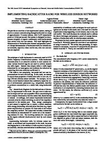
In chapter 2 are reported all the papers that show the work done in the context of the depicted scenario and the identified challenges. They contain all the details of the single parts briefly described in this chapter. Here the general scheme of the cognitive engine, object of this work, is presented and its system model is depicted. Every paper reported in chapter 2 covers an aspect of the cited challenges: each of them presents the problem (by always keeping in mind the cognitive network framework), explains the

CHAPTER 1. INTRODUCTION

16 application / traffic type

Networks recognition

active networks

Network selection

available networks

selected network

performance of selected network

Figure 1.1: System model of the cognitive engine proposed in this work. proposed solution, does some experimentations to test the effectiveness of the proposed method, presents and discusses the obtained results. Every paper is, therefore, part of a bigger scheme, and the conclusions obtained in each of these papers complete the puzzle and form a set of results that may be useful for continuing the research on cognitive radio and cognitive networks. Ideally, this work together with all the other studies done on this topic (and that are currently being done, since this topic is currently a really hot research topic) should form the basis and permit the practical realization of a real cognitive radio device, to be produced and sold on the market. By coming back to this work, the general scheme of the cognitive engine designed here can be represented by the system model shown in figure 1.1. It is composed by two main blocks connected to each other: • the networks recognition block; • the network selection block. The networks recognition block is thought to be provided by a simple energy detector, in line with the simplicity approach and coherently with what was exposed above. No single receivers for the different technologies (for example a Wi-Fi receiver, a Bluetooth receiver, . . . ) are thought to be present, therefore. As its name suggests, this block performs the networks recognition by using MAC layer features, as explained. The first three papers presented in chapter 2 are part of this block: they explain in details its behaviour and make experimentations on the proposed approach with MAC layer features. In particular, paper 2.1 presents in general the recognition and automatic classification with MAC layer features approach and performs classification

CHAPTER 1. INTRODUCTION

17

tests between Bluetooth and Wi-Fi. Paper 2.2 shows more tests that were carried out only on Bluetooth technology, with all real data effectively captured with the mentioned USRP as energy detector. In paper 2.3 the MAC layer features concept is extended to impulse radio UWB networks (as an example of underlay networks), whose much wider used band might cover and include the ISM 2.4 GHz unlicensed band, considered here. The output of this block is a list of all currently active networks in ISM 2.4 GHz band in the surrounding radio environment: they are all types of networks that present an ongoing communication at the moment of detection. The output of this block is directly passed to the next block. The network selection block is the core of the presented cognitive engine. Ideally this block presents a very generic hardware, i.e. it is composed by a software-defined radio. Again, the name of this block is auto-explicative: its task is, in fact, the selection of the wireless network present in that instant in the surrounding radio environment, that can offer the best QoE for the final user; it uses the KPIs approach following the method mentioned above and explained in more details in the papers in the following chapter. When the device must measure the performance of a network and when, instead, must use and exploit a network for communication purposes, this is controlled based on the studies done on MABs; therefore, the parameter that must be measured determines the reward PDF distribution, and this together with the available time horizon and the available hardware (basically its ability to perform measures in a relatively small time period) influences the choice on the MAB algorithm that must be chosen. The other three papers presented in chapter 2 describe different aspects of the behaviour of this block. Paper 2.4 introduces the concept of QoE and KPIs, explains the proposed approach and method and models the entire system. Paper 2.5 shows the first studies done on MAB in this context and scenario and introduces the new model with the difference between the two actions of measuring and using. It also presents the first experiments done on this. In paper 2.6 a refined and more complete model for MAB is proposed, and larger tests on the impact of its introduction are carried out, with more algorithms and different PDF distributions for the arms rewards. Note that this paper resumes many parts of paper 2.5 but extends them under the cited aspects. This block presents many inputs: • the application that the user has requested to run; • the available wireless networks; • the active networks; • the performance that the currently selected network is giving.

CHAPTER 1. INTRODUCTION

18

APPLICATION LAYER! Application! Available networks!

NETWORK SELECTOR!

Selected network!

LOWER LAYERS! Presentation! Session! Transport! Network! MAC & LLC! PHY!

Figure 1.2: Model of the network selector block, that emphasizes its position among the traditional OSI protocol stack model layers. The application that must be run is associated to a specific traffic type, which determines the KPIs of interest. The wireless networks available in the surrounding radio environment form the set of the arms (using MAB terminology) among which the choice must be done. Active networks come from the output of the networks recognition block. The last input is the feedback obtained from the selected network, as the MAB model provides, that contains the performance the network is currently providing (the current values of the parameters that were decided to be taken into consideration). The output is the wireless network selected for offering the best QoE to the user (given the application he has requested to run). The idea is that in practical implementation this output must be an input of the device operating system (OS), as also shown in figure 1.2. In fact the OS is the responsible of the task of automatically connecting to the selected network; in this way all the “radio environment adaptation” process of the device endowed with this cognitive engine is completely transparent for the user, who simply benefits of these choices and obtains the best experience he can have, given the condition, for its communication. Note that figure 1.2 shows the considered model of the network selector block and emphasizes its position among the traditional OSI protocol stack model layers. As last consideration, it should be noted that the network selection block should be built with an SDR, as mentioned; this means that every communication type is controlled by software. At the moment, however, devices provided with receivers for the different technologies (in particular Wi-Fi and UMTS receivers) were used instead of using an SDR; this was done in order to perform the practical experimentations with the available hardware. This does not influence nor substantially affect, however, the

CHAPTER 1. INTRODUCTION

19

general idea (in fact no concurrent measurements were provided, no measures were taken at the same time by exploiting the different receivers for the different technologies), and in future realizations of the cognitive engine only generic hardware must be used, as in the networks recognition block.

Chapter 2

Papers 2.1

Towards Cognitive Networking: Automatic Wireless Network Recognition Based on MAC Feature Detection

Abstract A cognitive radio device must be able to discover and recognize wireless networks eventually present in the surrounding environment. This chapter presents a recognition method based on MAC sub-layer features. Based on the fact that every wireless technology has its own specific MAC sub-layer behaviour, as defined by the technology Standard, network recognition can be reached by exploiting this particular behaviour. From the packet exchange pattern, peculiar of a single technology, MAC features can be extracted, and later they can be used for automatic recognition. The advantage of these “high-level” features, instead of physical ones, resides in the simplicity of the method: only a simple energy detector and low-complexity algorithms are required. In this chapter automatic recognition based on MAC features is applied at three cases of wireless networks operating in the ISM 2.4 GHz band: Bluetooth, Wi-Fi and ZigBee. Furthermore, this idea is extended to underlay networks such as Ultra Wide Band networks. A study-case is also presented that provides an illustration of automatic classification between Wi-Fi and Bluetooth networks.

This paper was published as chapter 9 in the Springer edited book Cognitive Radio and its Application for Next Generation Cellular and Wireless Networks.

20

CHAPTER 2. PAPERS

21

Chapter 9

Towards Cognitive Networking: Automatic Wireless Network Recognition Based on MAC Feature Detection Maria-Gabriella Di Benedetto and Stefano Boldrini

Abstract A cognitive radio device must be able to discover and recognize wireless networks eventually present in the surrounding environment. This chapter presents a recognition method based on MAC sub-layer features. Based on the fact that every wireless technology has its own specific MAC sub-layer behaviour, as defined by the technology Standard, network recognition can be reached by exploiting this particular behaviour. From the packet exchange pattern, peculiar of a single technology, MAC features can be extracted, and later they can be used for automatic recognition. The advantage of these ‘‘high-level’’ features, instead of physical ones, resides in the simplicity of the method: only a simple energy detector and low-complexity algorithms are required. In this chapter automatic recognition based on MAC features is applied at three cases of wireless networks operating in the ISM 2.4 GHz band: Bluetooth, Wi-Fi and ZigBee. Furthermore, this idea is extended to underlay networks such as Ultra Wide Band networks. A study-case is also presented that provides an illustration of automatic classification between Wi-Fi and Bluetooth networks.

9.1 Recognition of Wireless Technologies Present in the Environment: ISM 2.4 GHz Band As the cognitive radio appears to be an emergent and very promising device for the near future use [1], an important issue that needs to be solved rises up: the automatic recognition of wireless technologies eventually present in the surrounding environment. M.-G. Di Benedetto (&) ! S. Boldrini DIET Department, Spaienza University of Rome, Rome, Italy e-mail: [email protected] S. Boldrini e-mail: [email protected] H. Venkataraman and G.-M. Muntean (eds.), Cognitive Radio and its Application for Next Generation Cellular and Wireless Networks, Lecture Notes in Electrical Engineering 116, DOI: 10.1007/978-94-007-1827-2_9, ! Springer Science+Business Media Dordrecht 2012

239

CHAPTER 2. PAPERS 240

22 M.-G. Di Benedetto and S. Boldrini

In fact, nowadays a large amount of devices connect to each other wirelessly, using radio waves, and this number of devices is continuously growing. This means that if a cognitive radio wants to operate in a certain frequency band, it could be very common that other devices are still transmitting and receiving in the same band. In order not to interfere, or to exploit the unused frequency ranges, or just to be aware of the radio environment in which it is set, cognitive radio has to discover if other wireless networks are active in that moment in that place. This chapter aims to deal with this issue by proposing a method for automatic recognition and classification of wireless technologies. The considered frequency band is the Industrial Scientific and Medical (ISM) 2.4 GHz band. Many different and widespread networks operate in this band, that is open for use without any particular license: these two reasons make this band particularly appealing. Well-known examples of technologies operating in this band are: • Bluetooth (IEEE 802.15.1) [2]; • Wi-Fi (IEEE 802.11) [3]; • ZigBee (IEEE 802.15.4) [4]. ISM 2.4 GHz band is also exploited by many wireless mice and keyboards, cordless Wi-Fi phones and also by cameras for security closed-circuit TVs. Moreover, common interference at 2.4 GHz band comes from microwave ovens and DECT cordless phones (operating at 1.9 GHz); these can compromise the quality of the radio link of the other technologies, and should be also taken into account by the cognitive radio recognition system. Classification is very important for a cognitive radio device because it may be the initial step, through which it can be aware of the surrounding environment. In other words, if the cognitive is able to recognize and to classify the other wireless networks that are present, it can have a sort of ‘‘reaction’’, it can adapt its transmission and reception parameters and take ‘‘conscious’’ decisions, i.e. decisions based on the actual RF condition.

9.2 MAC Sub-Layer Features Exploitation As explained before, the goal of this chapter is to achieve automatic technologies recognition and classification in the framework of cognitive radio and cognitive networking. Many different approaches were used to obtain this goal. The most known is probably the spectrum sensing [5]. This approach, however, needs to use complex algorithms and high computational load [6–16]. The approach adopted in this chapter is also adopted by ‘‘AIR-AWARE’’, a project born at DIET Department (Department of Information, Electronic and Telecommunications engineering) of Sapienza University of Rome, and consists of exploiting features of the MAC sub-layer of the different wireless technologies. The idea that resides under this approach is that every network has its own

CHAPTER 2. PAPERS 9 Towards Cognitive Networking

23 241

Fig. 9.1 Graphical representation of the approach of the AIRAWARE project. Source [17]

particular and peculiar MAC behaviour, as expressed in the Standard that defines each technology. Based on the study of these Standards, a MAC peculiar behaviour can be identified for each type of network. Furthermore, some features that reflects these MAC behaviours can be found, and through these features, a recognition and classification process can be carried out. In particular, a time-domain packet diagram must be obtained. This diagram shows the presence versus absence of a packet in every instant. With the term ‘‘packet’’ in this chapter it is intended a MAC sub-layer information unit, that in some technologies is effectively called ‘‘packet’’, in some other ones ‘‘frame’’ or ‘‘datagram’’ or in other ways. Note that the content of these packets, i.e. which bits they are carrying, is not relevant for the scope of this recognition. What is important is only the packet pattern, that is whether a packet is present or not. An analysis of this packet exchange pattern can be very useful for revealing the technology that is currently in use, leading to network recognition. Let’s see this concept in a more detailed way. The Standard that defines a wireless technology deeply describes every aspect of its functionalities, and of course its MAC sublayer behaviour. This means that there can be maximum or minimum durations for certain types of packets, or even fixed durations. The same rules can be determined for the silence gaps that fall between the packets. Other rules that the Standard may specify can be a regular and predetermined transmission of a packet (usually these are control packets, that are needed for the correct system functionalities), or the transmission of acknowledgment packets after the reception of data packets. All these rules are specific for every single technology, i.e. each different network may present a MAC behaviour that is proper and peculiar of that technology. This means that an identification of each single behaviour can be useful for the identification of each technology, leading to the final goal of the network recognition. For this reason, based on the study of the Standard, some MAC features were identified for the three technologies taken into account: Bluetooth, Wi-Fi and ZigBee. These features can highlight the MAC specific behaviour and can be therefore exploited for recognition (Fig. 9.1). This approach integrates the cognitive concept at the network layer, having the big advantage, respect to the widely used spectrum sensing approach, of being extremely simple, and thus keeping a high computational efficiency. In fact, in order to obtain the mentioned time-domain packet exchange diagram, only a simple and ‘‘rudimentary’’ device is needed: an Energy Detector. Through this, the short-term

CHAPTER 2. PAPERS 242

24 M.-G. Di Benedetto and S. Boldrini

energy that is present on the air interface can be computed. After defining a threshold value, all the consecutive short-term energy values that are higher than the threshold can be considered as a packet. In this way, the packet diagram can be formed using energy detection. As for determining the threshold value, it is dependent from the device that is used and from the noise floor measured in ‘‘silence condition’’, i.e. when no other wireless device is transmitting [18]. The use of MAC features, despite the simplicity of the hardware needed and the low complexity of the algorithm used, proves to be quite accurate in simple scenarios, as will be presented later in this chapter. It can also be considered one among the possible classification strategies based on information from protocol layers above the physical one. In any case, in a more general view considering the context of cognitive radio, this can be a step inserted in the framework of a crosslayer cognitive engine. In other words, the recognition based on MAC features can be a first step (for its simplicity), that can also be refined using other layers features or other methods, increasing the correct network classification rate, but also increasing the complexity of the system and the computational load.

9.3 The Bluetooth Case The first analyzed technology is Bluetooth. It is defined in the IEEE Standard 802.15.1, that describes the specifications for the MAC and PHY layers, and it is used for Wireless Personal Area Networks (WPANs). This technology is nowadays available in quite every wireless device, such as cellular phones, laptops and netbooks, and for this reason it is very common to find an active Bluetooth device in many places. Bluetooth devices can communicate in the context of a piconet, that can be composed by 2–8 devices, all synchronized to a common clock and all sharing the same hopping sequence. In the piconet there is one device called master and the other devices are called slaves (up to 7). The master is the centre of the topology, that is to say that every slave communicates directly only with the master; in this way a communication between two slaves always passes through the master. The band used is the whole ISM 2.4 GHz band: from 2.4 to 2.4835 GHz. The bandwidth of the signal is in fact of 1 MHz, but the whole band is exploited by using the Frequency Hopping Spread Spectrum (FHSS) technique. The ISM band is therefore divided into 79 channels of 1 MHz each. The Gaussian Frequency Shift Keying (GFSK) modulation is used. Note that we took as reference the IEEE Standard 802.15.1—2005, that is the last IEEE available standard and that describes the version 1.2 of Bluetooth, providing a bitrate of 1 Mb/s. Later Bluetooth version was described in documents of the Bluetooth Special Interest Group (SIG). Very important for the scope of this chapter, is the division of the time axis into time slots. Every device has a clock with a period of 312.5 ls. A time slot duration

CHAPTER 2. PAPERS 9 Towards Cognitive Networking

25 243

of 625 ls is defined, that is two clock cycles, and the time axis is divided into time slots, all of this duration. Every packet transmission can start only at the beginning of a time slot. A packet can last an odd number of time slots; in particular, there can be 1-time slot packets, 3-time slots packets and 5-time slots packets. A communication between the master device and a slave device is usually composed by alternate packets (one from master and one from slave), since each device waits for a ‘‘return packet’’ (at least an acknowledgment) after sending a packet. Following these rules, imposed by the Standard, it is clear that a Bluetooth MAC packet exchange pattern is characterized by packets that start every time slot duration, or at multiples of this value, if considering the multi-slot packets. Furthermore, many acknowledgment packets are expected; the so called ‘‘NULL’’ packet is the one used for acknowledgment, and it has a fixed length of 126 bits, that corresponds to a fixed duration of 126 ls considering the bitrate of 1 Mb/s. The other packets have also minimum and maximum durations, imposed by the Standard. This rules’ set turns out into a Bluetooth peculiar pattern, that can be exploited through the use of features for the automatic recognition and classification. Possible MAC features are proposed later in the chapter. It is important to note that a Bluetooth communication system is dimensioned considering a bandwidth of 1 MHz in a single instant. By using an Energy Detector, the hopping sequence is unknown, and therefore it is impossible to know to which channel to be tuned to in every instant. In this condition, a simple way to catch the energy of all the packets that the devices send and receive is to sense the entire ISM 2.4 GHz band, i.e. all the 79 channels; by doing this, however, the noise power will be much higher, and this must be taken into account in the phase of determination of the threshold for the high versus low energy value. A possible alternative is to sense a lower bandwidth, in order to decrease the sensed noise power. In this way, however, all the packets sent in channels outside the sensed band are not caught. Considering that the ‘‘choice’’ to use a single channel has a uniform probability density, i.e. in mean there are no channels that are chosen more than others, sensing a lower bandwidth can still be a good tradeoff between considered bandwidth and ‘‘packet loss’’ (in sensing term).

9.4 The Wi-Fi Case The Wi-Fi technology is defined in the IEEE Standard 802.11; in particular the reference standard taken into account in this chapter is the revised version of 2007. There are different types of physical layers, each of them with a different used band, modulation transmission rates and coding; this results in different 802.11 Standard version (802.11a, b, c, d, e, f, g, h, i, j, k, n, p, r, s, v, w, y). The 802.11b version is considered in this chapter.

CHAPTER 2. PAPERS 244

26 M.-G. Di Benedetto and S. Boldrini

A Wi-Fi system consists basically in an Access Point (AP) to which single client devices are connected, and that gives access to a wider network (usually Internet); in this way a Wireless Local Area Network (WLAN) is created. The physical layer of a Wi-Fi network is different depending on the Standard version, of course, but obviously even for the supported bitrate, whose value can be variable. In particular, 802.11b uses the ISM 2.4 GHz band, with Direct Sequence Spread Spectrum (DSSS); possible birates are 1, 2, 5.5 and 11 Mb/s. The modulations used are the following: • Differential Binary Phase Shift Keying (DBPSK) for a bitrate of 1 Mb/s; • Differential Quadrature Phase Shift Keying (DQPSK) for a bitrate of 2 Mb/s; • Code Complementary Keying (CCK) for a bitrate of 5.5 and 11 Mb/s. Considering the MAC sub-layer, important for the scope of this chapter, the Distributed Coordination Function (DCF) is used, that employs a Carrier Sense Multiple Access with Collision Avoidance (CSMA/CA) access scheme. Furthermore, Request To Send—Clear To Send (RTS/CTS) mechanism is optionally adopted. Other enhances and improvements to these simple schemes in the medium access are also introduced, such as Enhanced Distributed Channel Access (EDCA) and Hybrid Coordination Function (HCF) Controlled Channel Access (HCCA). Different InterFrame Spaces (IFSs) are also defined. In particular, relevant for the purpose of the AIR-AWARE project, is the Short InterFrame Space (SIFS), the shortest of the IFSs. It is important for us because it is used before the transmission of an acknowledgment (ACK) packet or a CTS packet. It is defined as the time duration between the end of the last symbol of the previous packet and the beginning of the first symbol of the following packet, as seen at the air interface. Since the data-ACK packet exchange appears to be effectively really used, based on real traffic analysis in a scenario with medium to high traffic, the SIFS, among the different IFSs, is the most likely to occur. This is very important because it has a nominal value of 10 ls (even for the ‘‘g’’ and ‘‘n’’ versions of the Standard, in the 2.4 GHz band). This value of 10 ls is important in this context because it is a silence gap value that occurs very often in a Wi-Fi transmission and, most important, is peculiar of this technology, i.e. it characterizes this type of network. Thanks to this peculiarity, it can be a good candidate for being a feature.

9.5 The ZigBee Case ZigBee is defined in the IEEE Standard 802.15.4 (the version of 2006 is taken into account in this chapter) and it is designed for Low-Rate Wireless Personal Area Networks (LR-WPANs); in particular, physical and MAC layers are described and their behaviour is defined. This technology can operate in different frequency bands, and one among them is the ISM 2.4 GHz band, that is considered in this chapter.

CHAPTER 2. PAPERS 9 Towards Cognitive Networking

27 245

Based on the band used, the Standard defines different functionalities and transmission parameters. In the case of the 2.4 GHz band, a Direct Sequence Spread Spectrum (DSSS) technique is used, with an Offset-Quadrature Phase Shift Keying (O-QPSK) modulation. The data rate is 250 kb/s, that results in a 2 Mchips/s chip rate after the DSSS phase. 16 channels of 2 MHz each are defined, whose centre frequencies are separated of 5 MHz. As for the MAC sub-layer behaviour, there is a superframe, even if not mandatory, delimited by two beacons. The superframe is divided into two periods: the active one, where the devices can send and receive their packets, and the inactive one. Moreover, the active period is divided into two more parts: the Content Access Period and the Contention Free Period. The first one, that is divided into 16 slots of the same duration, uses a Carrier Sense Multiple Access with Collision Avoidance (CSMA/CA) access scheme, and therefore, as the name says, can be characterized by collisions. The Contention Free Period, that is optional, guarantees the absence of transmission collisions by defining Guaranteed Time Slots (GTSs), that can be in a maximum number of 7; every GTS can occupy more than one of the 16 slots defined for the whole active period (and mentioned before, with the Contention Access Period). The inactive period is optional, and can be used by ZigBee devices for entering low-power consumption functionalty modes. Even in ZigBee the packet transmission can be acknowledged, possibly resulting in a data-ACK packet exchange pattern. As in the other two wireless technologies, already described, also in ZigBee the InterFrame Spacing (IFS) is defined for temporarily separate two MAC frames (two MAC packets, in the mentioned notation used in this chapter) and permit the processing by the MAC sub-layer. There are two types of IFS: the Short IFS (SIFS) and the Long IFS (LIFS). Minimum durations are set by the Standard for both SIFS and LIFS. In particular, interesting for the purpose of this chapter and for this approach of automatic network recognition, it must be noted that the SIFS minimum value is 192 ls. This is extremely differentiated from the Wi-Fi case, where the SIFS has a nominal value of 10 ls. This difference in a value relative to the same silence gap, i.e. the SIFS, is very important for the scope of this project. In fact, this is a clear example of a difference MAC sub-layer behaviour in the same characteristic analyzed, and for this reason it could be a good candidate for a feature, because it can separate the two wireless technologies (Wi-Fi and ZigBee) by only considering this InterFrame Space, that is very simple to extract from a packet exchange diagram.

9.6 Extension to Underlay Networks: Ultra Wide Band Networks The concept that was explained can also be extended to other types of networks. Interesting is the case of underlay networks, that occupy a much higher bandwidth and a wider range of frequencies; these types of networks can be seen as a sort of

CHAPTER 2. PAPERS 246

28 M.-G. Di Benedetto and S. Boldrini

‘‘substrate’’ for the other wireless networks, and can also affect the recognition and classification process of the cognitive radio [19, 20]. An example is Ultra Wide Band (UWB) networks. This communication system is defined in IEEE Standard 802.15.4a, and uses impulse radio. In fact the duration of the pulses used in this technology is 700 ps to 1 ns; due to this really short duration, the occupied bandwidth is extremely high (some Gigahertz). The extension of the approach explained before, in order to reach automatic network recognition and classification, must not be intended in the sense of MAC sub-layer features. In fact the different bandwidth usage does not permit a direct comparison of this layer’s behaviour. Anyway the extension of the approach to this kind of networks is in the simplicity of the feature analysis that can be done. In this context, a physical layer feature can be used. The impulsive nature of this kind of signal can be exploited and compared to the continuous waveform signals used in traditional communication systems. This different nature can be shown through appropriate features, and therefore used for recognition. In particular, an analysis on the short-term energy can be a key operation, capable of highlight the difference between impulsive signals and continuous signals. In fact, continuous signals should present a constant energy profile (if the window used to measure the short-term energy is not exaggeratedly short, i.e. it contains at least a period of the transmitted signal), while the energy profile of a UWB signal should present many discontinuities, that depends on the fact that sometimes the window used to measure the short-term energy includes one (or more) pulse, and sometimes not. Obviously the short-term energy windowing must be sufficiently short, otherwise, a mean value of many pulses is obtained, not reflecting the impulsive nature of the signal. Preliminary studies on constant versus impulsive energy profiles were carried out until now, in which Bluetooth was used as example of continuous signal network. Short-term energy was computed for both signals, the impulsive one and the continuous one, using different values of window duration. Considering the Bluetooth continuous-wave signal, it can be seen that the wider the window width, the smaller the fluctuation of the short-term energy gets: as the window width increases, the short-term energy becomes flatter. An example is shown in Fig. 9.2. Analyzing the short-term energy profile of the UWB signal, it clearly appears very different: with a short window width it has impulsive nature, shown by the presence of peaks; as the width of the window increases, it does not assume a smoother behaviour, as in the previous case, but it presents even higher peaks, as it can be seen in Figs. 9.3 and 9.4. Furthermore, short-term energy appears extremely concentrated in very few discrete values. Even if these first results are still preliminary, and deeper studies need to be done under this aspect, it can be seen that, with a proper window width, the shortterm energy of a continuous waveform (Bluetooth, in this case) is approximately flat, while the one of an impulsive signal (UWB) is multi-static and very discontinuous. Most important, they are clearly very different. This difference could be exploited for the UWB network detection.

CHAPTER 2. PAPERS 9 Towards Cognitive Networking

29 247

Fig. 9.2 Short-term energy of a Bluetooth signal, function of time and window width. Source [21] Fig. 9.3 Short-term energy of a UWB signal, with a window width equal to 1 pulse duration. Source [21]

This example follows the approach indicated from the beginning of this chapter, since only simple operations, with very low complexity, are executed. In other words, through simple features, of physical layer in this case, it seems possible to reach network detection and recognition.

9.7 Recognition and Automatic Classification After this brief analysis of the technologies operating in the ISM 2.4 GHz band, and the extension to the UWB underlay network, some MAC sub-layer features are proposed, with the purpose of reaching the wireless network recognition and automatic classification.

CHAPTER 2. PAPERS 248

30 M.-G. Di Benedetto and S. Boldrini

Fig. 9.4 Short-term energy of a UWB signal, with a window width equal to 10 pulse duration. Source Ref. [21]

As for Bluetooth, the presented features are the following two: • packet duration; • packet inter-arrival interval. The reason for the choice of these features resides in the fact that they reflect some behaviours peculiar of Bluetooth [22]. In fact, as explained before, acknowledgment packets are very common in the packet exchange pattern, and the NULL packet, used for the acknowledgment, has a fixed duration of 126 ls. Furthermore, it can be expected that, if large amount of data must be sent, packets are filled efficiently as much as they can; in this way, they often reach their maximum length, i.e. their maximum duration. As defined in the Standard, maximum duration are: 366 ls for 1-time slot packets, 1622 ls for 3-time slot packets, and 2870 ls for 5-time slots packets. Some fixed, minimum and maximum duration values defined in the Standard are reported in Table 9.1. For these reasons, these maximum and fixed values of packet durations, specific of this technology, may occur very often in a Bluetooth communication. Moreover, if during a ‘‘blind’’ packet sensing operation (i.e. without knowing which network is active and transmitting), these values of packet durations are met frequently, they can be the sign of the presence of a Bluetooth network. The packet inter-arrival interval feature is chosen given that Bluetooth provides a slotted communication, with a time slot duration of 625 ls that is peculiar of this technology. When the ‘‘blind’’ sensed packet exchange pattern presents a value of 625 ls (or its multiples, considering multi-slots packets and ‘‘packet loss’’ if sensing a bandwidth lower than the whole ISM band) for the packet inter-arrival interval, the probability that these sensed packets are Bluetooth packets is reasonably high.

CHAPTER 2. PAPERS

31

9 Towards Cognitive Networking

249

Table 9.1 Bluetooth packet durations, as defined by the Standard Fixed duration (ls) Min duration (ls)

Max duration (ls)

Time slot NULL packet (ACK) 1-TS packet 3-TSs packet 5-TSs packet

– – 366 1622 2870

625 126 – – –

– – 126 1250 2500

Source [17]

In the Wi-Fi case, based on the analysis of its MAC behaviour presented above, the following two features are considered: • duration of silence gaps identified as SIFS; • duration of the longest packet, considering all the packets between two consecutive silence gaps previously identified as SIFS. The first feature was proposed based on the fact that the exchange of a data packet followed by an acknowledgment packet is very common. These two packets are therefore separated by a silence gap defined as SIFS, whose duration is fixed by the Wi-Fi Standard at 10 ls. This value is characteristic for Wi-Fi, and therefore if such a value is found in the analysis of this feature, it probably means that the packet exchange pattern is one of a Wi-Fi communication. The second feature was chosen because the longest packet in a block delimited by two SIFS should present a value range quite restricted, in which the contained values may be quite different from the ones encountered in a Bluetooth communication. Even this feature can, therefore, be useful for Wi-Fi automatic recognition. None features specific for ZigBee were selected until now. The reason for this is that the already identified features seem to permit the classification of these three technologies, by identifying the behaviour of one particular network and excluding the others. If these features can lead to automatic recognition, with a reasonably high correct classification rate, there is no need to add other features. Furthermore, it must be remembered that one primary objective is to maintain the system as simple as possible. In order to perform a more reliable classification, other features can be added later, even specific for ZigBee; this in analogy with the cross-layer cognitive engine point of view. An important aspect that must be observed is that all these features are very simple to extract from the packet exchange diagram, and are also simple to analyze, requiring low computational load and algorithms. This is really important, remembering the AIR-AWARE projects aims. Also note that the selected features were identified independently from the others, based on the Standard definitions and on the technologies behaviours. This implies that the features may be correlated. In general, the adopted approach may be prone to this fact. Anyway it can be avoided in an optimization step, after every feature proposal, in order to get the minimum numbr of features necessary to obtain a predefined correct classification rate. In this way, all the correlated

CHAPTER 2. PAPERS 250

32 M.-G. Di Benedetto and S. Boldrini

features can be discarded, as well as the features that prove to obtain less significant improvements in the classification. Or they can be used in a secondary step, to improve the initial classification, if desired, without giving too much unnecessary load at first. All the selected features are therefore used for classification. In particular, after choosing the desired classifier, they take part in the classifier’s training phase, in order to fit the classifier’s parameteres. This training phase must obviously be done by applying the features to a packet exchange pattern coming from a known network, in order to indicate that the obtained features values are peculiar of that specific technology. This training must be done with all the decided features, and for all the technologies that are considered. After the training step, the trained classifier is ready to perform its automatic network recognition and classification. It must be noticed that all this procedure is extremely simple: it requires simple hardware and has a very low computational cost. This is very important in terms of practical realization of this scheme in a real cognitive radio device. In fact, by using the proposed scheme and procedure implemented in a cognitive radio, it can be aware of the other wireless networks without the need of complex spectrum analysis, but exploiting the benefits of simplicity introduced by this approach. This can result in a more simple device, and can also permit its realization with low cost, that is always an important aspect marketing.

9.8 Study-Case: Wi-Fi Versus Bluetooth Automatic Classification After presenting the AIR-AWARE project, its objectives, the MAC sub-layer features, the wireless technologies that are considered, and the selected features, a study-case is proposed: Wi-Fi versus Bluetooth automatic classification. This example is presented in order to show how this approach can be carried out in practice. For this reason, a simple scenario is taken into account, by considering only two technologies (the two ones mentioned above: Wi-Fi and Bluetooth) and by exploiting only the two proposed features specific for Wi-Fi, i.e.: • duration of silence gaps identified as SIFS; • duration of the longest packet, considering all the packets between two consecutive silence gaps previously identified as SIFS. In order to extract the SIFSs, differentiating them from the non-SIFS silence gaps, the following rule was adopted: a silence gap was considered as SIFS if the duration of the 60% of the ith packet was higher than the duration of the whole ith ? 1 packet: 0:6" p#durationi [ p#durationiþ1:

CHAPTER 2. PAPERS 9 Towards Cognitive Networking

33 251

This is based on the consideration that a SIFS separates a data packet (preceding) from an acknowledgement packt (following), and that a data packet is considerably longer than an acknowledgement one. The Wi-Fi traffic, i.e. the Wi-Fi packet exchange diagram, is real traffic obtained through a ‘‘Sniffer Station’’, a packet capturing device. This device is a personal computer with a real-time kernel Operating System, running a packet capturing application, specifically developed, and with a Network Wireless Adapter turned into ‘‘monitor mode’’. The ‘‘monitor mode’’ allows to intercept every packet within the receiver’s range (and not only those directed to the device, as happens with the Network Wireless Adapter in ‘‘normal mode’’). The packet capturing application and the real-time kernel permit to obtain the whole packets with accurate time-stamps, i.e. arrival times. The packet traffic was generated by three other personal computers tuned to an Access Point, in different conditions of traffic load (low, medium and high packet exchange number). As for the Bluetooth traffic, the packet exchange pattern was obtained using " simulated packets, generated using MATLAB . Two Bluetooth devices are considered, a master and a slave, who send their packets alternately, performing a data-ACK exchange: every packet sent receives an acknowledgement. The simulated data packets are of all the three types: 1, 3 and 5 time-slot packets, depending on their length. For the acknowledgment the NULL packet is used, whose duration is 126 ls. Based on the Standard specifications, a jitter of ±10 ls on the arrival time is considered; the jitter was modeled by a Gaussian distribution, with zero mean standard deviation r = 10/3 ls. After the feature extraction, a block of packets results in a point in the 2-dimensions features space (two features were considered), as it can be seen in Fig. 9.5, where only single-slot Bluetooth packets are used, and in Fig. 9.6, where multi-slot Bluetooth packets are used. Four linear classifiers were used in this study-case: • • • •

Perceptron; Pocket; Least Mean Squares method (LMS); Sum Of Errors squares estimation (SOE).

The choice to use linear classifiers, and not more complex ones, capable of granting better performance, is always in order to keep the system as simple as possible. More complex classifiers can be added later to perform a more accurate classification, if necessary and desired [23, 24]. The explanation of how these classifiers work is out of the scope of this chapter, but they are very simple as well known, so they can be easily found. Anyway, just to mention the principles of classification they all share (without being exhausting, of course), their aim is to divide the F-dimensional features space into C classes, where F is the number of features and C is the number of classes. The division is reached through the computation for every class of discriminant functions gi that characterize the region of the F-dimensional space where each class is located:

CHAPTER 2. PAPERS

34

252

M.-G. Di Benedetto and S. Boldrini

Fig. 9.5 Features space with single-slot Bluetooth packets. Source [17]

Fig. 9.6 Features space with multi-slot Bluetooth packets. Source [17]

gi ðxÞ ¼ w0;i þ

F X j¼1

wj;i xj ; i ¼ 1; . . .; C

where w = [w0, w1, …, wF] is called the ‘‘weight vector’’ and x = [x1, …, xF] is a point in the features space. The difference among the four used classifiers is how they compute the discriminant functions gi, i.e. how they compute the weight vector w based on the training points x. The extracted features were used for the classifiers training. The trained linear classifiers results, therefore, as straight lines in the features space. Figures 9.7 and 9.8 show the features space already shown in Figs. 9.5 and 9.6, but with the trained linear classifiers.

CHAPTER 2. PAPERS 9 Towards Cognitive Networking

35 253

Fig. 9.7 Features space with single-slot Bluetooth packets and trained classifiers. Source [17]

Fig. 9.8 Features space with multi-slot Bluetooth packets and trained classifiers. Source [17]

As it can be seen, since the two classes (Wi-Fi and Bluetooth) are not separable in the case of multi-slot Bluetooth packets (Fig. 9.8), the classifiers will commit some errors in the classification phase. Perceptron and Pocket graphically seem to separate better the two classes, and it can be expected that these two classifiers will obtain better classification results than LMS and SOE. The classifiers were used for classification tests, using other packet exchange patterns, i.e. not belonging to the training set. Results of these tests are reported in Tables 9.2 (Bluetooth single-slot packets case) and 9.3 (Bluetooth multi-slot packets case). These results clearly show that the correct classification rate is perfect for all the four considered classifiers in the Bluetooth single-slot packets case, where the two

CHAPTER 2. PAPERS

36

254

M.-G. Di Benedetto and S. Boldrini

Table 9.2 Classification test results, Bluetooth single-slot packets Classifier Input network Classification into Wi-Fi Perceptron Perceptron Pocket Pocket LMS LMS SOE SOE

Wi-Fi Bluetooth Wi-Fi Bluetooth Wi-Fi Bluetooth Wi-Fi Bluetooth

100% [352/352] 0% [0/456] 100% [352/352] 0% [0/456] 100% [352/352] 0% [0/456] 100% [352/352] 0% [0/456]

Classification into single-slot Bluetooth 0% [0/352] 100% [456/456] 0% [0/352] 100% [456/456] 0% [0/352] 100% [456/456] 0% [0/352] 100% [456/456]

Source [17]

Table 9.3 Classification test results, Bluetooth multi-slot packets Classifier Input network Classification into Wi-Fi Perceptron Perceptron Pocket Pocket LMS LMS SOE SOE

Wi-Fi Bluetooth Wi-Fi Bluetooth Wi-Fi Bluetooth Wi-Fi Bluetooth

98.86% [348/352] 0.43% [2/462] 98.86% [348/352] 0% [0/462] 99.43% [350/352] 34.85% [161/462] 99.72% [351/352] 29.87% [138/462]

Classification into multi-slot Bluetooth 1.14% [4/352] 99.57% [460/462] 1.14% [4/352] 100% [462/462] 0.57% [2/352] 65.15% [301/462] 0.28% [1/352] 70.13% [324/462]

Source [17]

Table 9.4 Classification test results, multi-network environment Classifier Input network Classification into Wi-Fi Perceptron Perceptron Perceptron Pocket Pocket Pocket LMS LMS LMS SOE SOE SOE Source [17]

Wi-Fi predominant Bluetooth predominant Balanced Wi-Fi predominant Bluetooth predominant Balanced Wi-Fi predominant Bluetooth predominant Balanced Wi-Fi predominant Bluetooth predominant Balanced

86.07% [315/366] 17.22% [134/778] 41.53% [211/508] 86.07% [315/366] 17.1% [133/778] 41.34% [210/508] 90.16% [330/366] 37.79% [294/778] 56.89% [289/508] 90.71% [332/366] 36.89% [287/778] 56.1% [285/508]

Classification into multi-slot Bluetooth 13.93% [51/366] 82.78% [644/778] 58.47% [297/508] 13.93% [51/366] 82.9% [645/778] 58.66% [298/508] 9.84% [36/366] 62.21% [484/778] 43.11% [219/508] 9.29% [34/366] 63.11% [491/778] 43.9% [223/508]

CHAPTER 2. PAPERS 9 Towards Cognitive Networking

37 255

classes (Wi-Fi and Bluetooth) are separable. Correct classification rate cannot be perfect in the second case (Bluetooth multi-slot packets), since the packets are not separable, but it is still really high, very close to 100%, for all the classifiers. The obtained classification test results, even for a simple case reported here as an example, show that the approach adopted in the AIR-AWARE project and explained in this chapter is valid, because very high correct classification rates can be obtained only through features simple to extract and simple algorithms. In order to recreate a possible real multi-network scenario, multi-network packet traffic was generated, by mixing the two mentioned test sets. Furthermore, three different scenarios were considered: • Wi-Fi as predominant network, i.e. the number of Wi-Fi packets is higher than the Bluetooth one (1000 Wi-Fi packets vs. 200 Bluetooth packets); • Bluetooth as predominant network, i.e. the number of Bluetooth packets is higher than the Wi-Fi one (2000 Bluetooth packets vs. 1000 Wi-Fi packets); here only multi-slot Bluetooth packets are used, since this case is more general; • balanced scenario, i.e. the number of Wi-Fi packets is the same of the Bluetooth one (1000 Wi-Fi packets vs. 1000 Bluetooth packets). Table 9.4 reports the obtained results for this case. Pocket and Perceptron classifiers, despite their simplicity, seem to obtain the best results, by always reaching a correct classification rate higher than 80% in case one network is predominant respect the other one. LMS and SOE reach a correct classification rate higher than 90% when Wi-Fi is predominant, but this rate is lower (about 60%) when the predominant network is Bluetooth. In the balanced scenario the correct classification rate is lower, but it should be noted that by obtaining rates close to 50%, it reflects the situation of the environment, where two different types of wireless networks are present ‘‘with the same percentage’’, i.e. their presence is balanced. In this case there could be the necessity to perform more investigation, for example with more features or using a cross-layer cognitive engine, i.e. with additional information coming from other architectural layers. This seem not necessary in the two scenarios where a technology is predominant to the other one; in these cases the MAC sub-layer features exploitation seem to lead to an automatic network correct classification with a high percentage. This means that it is reached only by exploiting very simple features and algorithms, that is the goal of the AIR-AWARE project.

References 1. Mitola J III, Maguire GQ Jr (1999) Cognitive radio: making software radios more personal. IEEE Pers Commun 6(4):13–18. doi:10.1109/98.788210 2. IEEE Standard for Information Technology-Telecommunications and Information Exchange Between Systems-Local and Metropolitan Area Networks-Specific Requirements-Part 15.1: Wireless Medium Access Control (MAC) and Physical Layer (PHY) Specifications for Wireless Personal Area Networks (WPANs), IEEE Std 802.15.1-2005 (Revision of IEEE Std 802.15.1-2002), pp 0_1-580, 2005. doi: 10.1109/IEEESTD.2005.96290

CHAPTER 2. PAPERS 256

38 M.-G. Di Benedetto and S. Boldrini

3. IEEE Standard for Information Technology-Telecommunications and Information Exchange Between Systems-Local and Metropolitan Area Networks-Specific Requirements-Part 11: Wireless LAN Medium Access Control (MAC) and Physical Layer (PHY) Specifications, IEEE Std 802.11-2007 (Revision of IEEE Std 802.11-1999), pp C1-1184, June 12 2007. doi: 10.1109/IEEESTD.2007.373646 4. IEEE Standard for Information Technology-Telecommunications and Information Exchange Between Systems-Local and Metropolitan Area Networks-Specific Requirements Part 15.4: Wireless Medium Access Control (MAC) and Physical Layer (PHY) Specifications for LowRate Wireless Personal Area Networks (WPANs), IEEE Std 802.15.4-2006 (Revision of IEEE Std 802.15.4-2003), pp 0_1-305, 2006. doi: 10.1109/IEEESTD.2006.232110 5. Haykin S, Thomson DJ, Reed JH (2009) Spectrum sensing for cognitive radio. Proc IEEE 97(5):849–877. doi:10.1109/JPROC.2009.2015711 6. Ghasemi A, Sousa ES (2008) Spectrum sensing in cognitive radio networks: requirements, challenges and design trade-offs. IEEE Commun Mag 46(4):32–39. doi:10.1109/MCOM. 2008.4481338 7. Yucek T, Arslan H (2009) A survey of spectrum sensing algorithms for cognitive radio applications. IEEE Commun Surv Tutor 11(1):116–130, First quarter 2009. doi: 10.1109/SURV. 2009.090109 8. Cabric D, Mishra SM, Brodersen RW (2004) Implementation issues in spectrum sensing for cognitive radios. In: Conference record of the thirty-eighth Asilomar conference on signals, systems and computers, vol 1, 7–10 Nov 2004, pp 772–776. doi: 10.1109/ACSSC.2004. 1399240 9. Liang Y-C, Zeng Y, Peh ECY, Hoang AT (2008) Sensing-throughput tradeoff for cognitive radio networks. IEEE Trans Wireless Commun 7(4):1326–1337. doi:10.1109/TWC.2008. 060869 10. Lee W-Y, Akyildiz IF (2008) Optimal spectrum sensing framework for cognitive radio networks. IEEE Trans Wireless Commun 7(10):3845–3857. doi: 10.1109/T-WC.2008.070391 11. Zeng Yonghong, Liang Ying-Chang (2009) Spectrum-sensing algorithms for cognitive radio based on statistical covariances. IEEE Trans Veh Technol 58(4):1804–1815. doi:10.1109/ TVT.2008.2005267 12. Chen Z, Guo N, Qiu RC (2010) Demonstration of real-time spectrum sensing for cognitive radio. In: Military communications conference, MILCOM 2010, Oct 31 2010–Nov 3 2010, pp 323–328. doi: 10.1109/MILCOM.2010.5680333 13. Zeng Y, Liang Y (2009) Eigenvalue-based spectrum sensing algorithms for cognitive radio. IEEE Trans Commun 57(6):1784–1793. doi:10.1109/TCOMM.2009.06.070402 14. Do T, Mark BL (2010) Joint spatial—temporal spectrum sensing for cognitive radio networks. IEEE Trans Vehicular Technol 59(7):3480–3490. doi:10.1109/TVT.2010.2050610 15. Filo M, Hossain A, Biswas AR, Piesiewicz R (2009) Cognitive pilot channel: Enabler for radio systems coexistence. In: Second international workshop on cognitive radio and advanced spectrum management, (CogART 2009), pp 17–23. doi: 10.1109/COGART.2009.5167226 16. Ishizu K, Murakami H, Harada H (2011) Feasibility study on spectrum sharing type cognitive radio system with outband pilot channel. In: 2011 sixth international ICST conference on cognitive radio oriented wireless networks and communications (CROWNCOM), pp 286–290 17. Di Benedetto M-G, Boldrini S, Martin Martin CJ, Roldan Diaz J (2010) Automatic network recognition by feature extraction: a case study in the ISM band. In: 2010 Proceedings of the fifth international conference on cognitive radio oriented wireless networks and communications (CROWNCOM), pp 1–5, 9–11. doi: 10.4108/ICST.CROWNCOM2010.9274 18. Zhuan Y, Memik G, Grosspietsch J (2008) Energy detection using estimated noise variance for spectrum sensing in cognitive radio networks. In: Proceedings of IEEE wireless communications and networking conference, WCNC 2008, March 31 2008–April 3 2008, pp 711–716. doi: 10.1109/WCNC.2008.131 19. Di Benedetto M-G, Giancola G (2004) Understanding ultra wide band radio fundamentals, 1st edn. Prentice Hall PTR, Englewood Cliffs. ISBN: 0-13-148003-0

CHAPTER 2. PAPERS 9 Towards Cognitive Networking

39 257

20. Francone M, Domenicali D, Di Benedetto M-G (2006) Time-varying interference spectral analysis for Cognitive UWB networks. In: 32nd annual conference on IEEE industrial electronics, IECON 2006, 6–10 Nov 2006, pp 3205–3210. doi: 10.1109/IECON.2006.348076 21. Boldrini S, Ferrante GC, Di Benedetto M-G (2011) UWB network recognition based on impulsiveness of energy profiles. In: 2011 IEEE international conference on ultra-wideband (ICUWB), 14–16 Sept 2011, pp 327–330. doi: 10.1109/ICUWB.2011.6058856 22. Benco S, Boldrini S, Ghittino A, Annese S, Di Benedetto M-G (2010) Identification of packet exchange patterns based on energy detection: the Bluetooth case. In: 2010 3rd international symposium on applied sciences in biomedical and communication technologies (ISABEL), 7–10 Nov 2010, pp 1–5. doi: 10.1109/ISABEL.2010.5702776 23. Theodoridis S, Koutroumbas K (2009) Pattern recognition, 4th edn. Elsevier Academic Press, New York. ISBN: 978-1-59749-272-0 24. Gallant SI (1990) Perceptron-based learning algorithms. IEEE Trans Neural Netw 1(2): 179–191. doi:10.1109/72.80230

CHAPTER 2. PAPERS

2.2

40

Bluetooth automatic network recognition – the AIR-AWARE approach

Abstract Automatic network recognition and classification may prove to be an important concept in the framework of cognitive radio and networks. For practical implementations, these operations must be carried out in a simple way by using simple devices and algorithms that require low computational load. The AIR-AWARE approach proposes to use MAC sub-layer features for technology recognition purposes where a rudimentary device like an energy detector is used for technology-specific feature extraction. The aim of this work is automatic Bluetooth classification. To this purpose, two MAC features reflecting properties, related to the time-varying pattern of MAC packet exchanges, are proposed. Experimental data obtained by using the Universal Software Radio Peripheral as energy detector show that the two proposed features are capable of highlighting MAC sub-layer behaviour peculiar to Bluetooth. These features may therefore lead to successful Bluetooth recognition and the results obtained provide support to the validity of the AIR-AWARE approach.

This paper was accepted for publication in the International Journal of Autonomous and Adaptive Communications Systems (IJAACS), Inderscience Publishers.

CHAPTER 2. PAPERS Int. J. Autonomous and Adaptive Communications Systems, Vol. x, No. x, xxxx

Bluetooth automatic network recognition – the AIR-AWARE approach Stefano Boldrini* Sapienza University of Rome, School of Engineering, DIET Department, Via Eudossiana, 18-00184 Rome, Italy E-mail: [email protected] *Corresponding author

Sergio Benco, Stefano Annese and Andrea Ghittino CSP s.c. a r.l. ‘ICT-Innovation’, Via Livorno, 60-10144 Turin, Italy E-mail: [email protected] E-mail: [email protected] E-mail: [email protected]

Maria-Gabriella Di Benedetto Sapienza University of Rome, School of Engineering, DIET Department, Via Eudossiana, 18-00184 Rome, Italy E-mail: [email protected] Abstract: Automatic network recognition and classification may prove to be an important concept in the framework of cognitive radio and networks. For practical implementations, these operations must be carried out in a simple way by using simple devices and algorithms that require low computational load. The AIR-AWARE approach proposes to use MAC sub-layer features for technology recognition purposes where a rudimentary device like an energy detector is used for technology-specific feature extraction. The aim of this work is automatic Bluetooth classification. To this purpose, two MAC features reflecting properties, related to the time-varying pattern of MAC packet exchanges, are proposed. Experimental data obtained by using the Universal Software Radio Peripheral as energy detector show that the two proposed features are capable of highlighting MAC sub-layer behaviour peculiar to Bluetooth. These features may therefore lead to successful Bluetooth recognition and the results obtained provide support to the validity of the AIR-AWARE approach. Keywords: cognitive networking; network discovery; automatic network classification; energy detection; USRP; universal software radio peripheral; Bluetooth automatic recognition; adaptive communications systems. Reference to this paper should be made as follows: Boldrini, S., Benco, S., Annese, S., Ghittino, A. and Di Benedetto, M-G. (xxxx) ‘Bluetooth automatic Copyright © 20xx Inderscience Enterprises Ltd.

41 1

CHAPTER 2. PAPERS 2

S. Boldrini et al. network recognition – the AIR-AWARE approach’, Int. J. Autonomous and Adaptive Communications Systems, Vol. x, No. x, pp.xx–xx. Biographical notes: Stefano Boldrini obtained his Bachelor’s degree in Telecommunications Engineering in 2006 from University of Trento and his Master of Science in Telecommunications Engineering in 2010 from Sapienza University of Rome. Currently, he is a PhD student in Information and Communication Engineering at Sapienza University of Rome, and his main research topics are cognitive radio and cognitive networking, with particular focus on automatic wireless network recognition and classification. Sergio Benco received his Bachelor’ degree and Master of Science in Telecommunication Engineering from Sapienza University of Rome, Italy, in 2006 and 2010, respectively. In 2010, he obtained a research grant from CSP – ICT Innovation focused on automatic wireless network recognition. He is currently working as a Consultant Engineer in the INLAB group (CSP – ICT Innovation) and as affiliated researcher in the ACTS lab of Sapienza University of Rome, DIET department. His research activities focus on spectrum sensing techniques for software defined radio. Stefano Annese received the Telecommunication Engineering degree from the Politecnico di Torino, Italy, in 2004. Since then he works for CSP – ICT Innovation as Junior Researcher and then as a Senior Resercher on broadband wireless technologies. He is currently the Integrated Networks Laboratory Manager in the Research and Development department. His research activities are focused on the first three layers protocols in wireless networks. He is the co-author of one patent. Andrea Ghittino received the Telecommunication Engineering degree (summa cum laude) from the Politecnico di Torino, Italy, in 2000. He works for CSP – ICT Innovation since then and he is currently the Networks and Wireless Communications Area Manager in the Research and Development department. His research activities are focused on protocols and quality of service management in wireless networks. He is the co-author of one patent. Maria-Gabriella Di Benedetto obtained her PhD in Telecommunications in 1987 from Sapienza University of Rome, Italy. In 1991, she joined the Faculty of Engineering of Sapienza University of Rome, where currently she is a Full Professor of Telecommunications. She has held visiting positions at the MIT, the University of California, Berkeley, and the University of Paris XI, France. In 1994, she received the Mac Kay Professorship award from the University of California, Berkeley. Her research interests include wireless communication systems and speech. From 1995 to 2000, she directed four European projects on UMTS design. Since 2000, she has been active in fostering the development of UWB communications in Europe, and recently increased activity in cognitive networks. She currently coordinates COST Action IC0902 and participates in the Network of Excellence ACROPOLIS. In October 2009, she received the Excellence in Research award ‘Sapienza Ricerca’, under the auspices of President of Italy.

42

CHAPTER 2. PAPERS Bluetooth automatic network recognition – the AIR-AWARE approach

43 3

In October 2009, she received the Excellence in Research award ‘Sapienza Ricerca’, under the auspices of President of Italy, Giorgio Napolitano. Portions of the data reported here were presented at the Third International Workshop on Cognitive Radio and Advanced Spectrum Management – CogART 2010, as published in Benco et al. (2010), that received the CogART 2010 Best Paper Award.

1

Introduction

An important concept in the context of cognitive radio and cognitive networking is wireless network recognition. In fact, a cognitive radio, in order to adapt and reconfigure its parameters based on the environment in which it is set, must be able to recognise the environment, i.e. to determine if there are other active wireless networks in that precise instant in that area. This is, therefore, a problem of wireless network detection and recognition. The AIR-AWARE Project, ‘born’ at the DIET Department of Sapienza University of Rome, and first mentioned in (Di Benedetto et al., 2010), addresses this problem. The main scope of this project is to reach automatic network recognition and classification in a simple way, by using simple devices and algorithms that require a low computational load. This keyword, simple, was practiced in the AIR-AWARE Project using MAC sub-layer features. In fact, every wireless network presents a MAC behaviour that is defined by its own standard and, most important, that is characteristic and peculiar of that single technology. This implies that an analysis of packet exchange patterns can reveal the tecnology present over the air at a certain time, leading to network recognition. To do so, it is therefore necessary to identify MAC features for each wireless technology. To keep the AIR-AWARE module as simple as possible, a ‘rudimentary’ device must be used for feature detection. Therefore, this project intends to use an energy detector (ED) in order to obtain, through sensing and calculation of the short-term energy, a time-domain packet diagram. The industrial, scientific and medical (ISM) 2.4 GHz unlicensed band is the most widely used band for a lot of widespread wireless technologies. Examples are Wi-Fi (IEEE Standard 802.11, 2007), Bluetooth (IEEE Standard 802.15.1, 2005) and ZigBee (IEEE Standard 802.15.4, 2006). In this work, the Bluetooth technology was analysed, and two MAC sub-layer features were identified that can highlight and distinguish this type of network among others in the same frequency band. The universal software radio peripheral (USRP) software defined radio (SDR) was used as ED in order to obtain the necessary packet diagram. Using these simple device and recognition procedures, an identification of packet exchange patterns specific of Bluetooth was carried out. The paper is organised as follows. Section 2 defines energy detection and explains how packet diagrams were obtained based on time-varying energy profiles. Section 3 contains a brief overview of Bluetooth technology, the analysis of its MAC behaviour, the proposed features and how they were applied to the case under analysis. In Section 4, the USRP platform and the experimental set-up are presented. Results of experimentation are presented in Section 5, while Section 6 contains a discussion of the results obtained and future directions of this research investigation.

CHAPTER 2. PAPERS 4

2

44

S. Boldrini et al.

Energy detection and packet diagrams

In the general framework of spectrum sensing, the ED approach has gained great interest due to its flexibility and relative low complexity (Mariani et al., 2010). The ED is based on the computation of received energy in a predefined time window (averaged over N samples of received signal). This operation gives rise to a sequence of energy values that we indicate as energy samples. These energy samples are then compared against a threshold that depends on noise level. Note that energy detection does not require any prior knowledge on spectrum occupancy, and this provides a beneficial flexibility towards wireless technology identification. Detection of random signals in presence of additive white Gaussian noise (AWGN) is a traditional problem that has been solved by detection theory. Under the hypothesis that the useful signal is unknown and is modelled as a zero-mean wide-sense stationary (WSS) Gaussian process with variance σs2 , whereas noise is AWGN with variance σw2 , the sufficient statistic T (r), i.e. the expression of ED input–output characteristic, is: T (r) =

N ! n=1

|rn |2

(1)

In Equation (1), r represents the received vector of complex samples rn and N the number of samples used in each energy calculation (i.e. window length). The window length N must be selected based on a trade-off between resolution in average energy vs. time-varying energy patterns. The short-term energy function is obtained from the product of Equation (1) by the ED sampling period Ts , where NTs = window duration, i.e. EN (r) =

N ! n=1

|rn |2 Ts

(2)

Since the sampling frequency was 25 MHz (as further described in Section 4), the sampling period was Ts = 40 ns. Based on Bluetooth packet duration, as explained later in Section 3, a reasonable window duration was 10 µsec, and therefore, in order to obtain this value, a rectangular window N of 250 samples was used. This number of samples offers a good trade-off between EN values and average values. In other words, N value is not ‘too high’, otherwise EN would be computed considering too many samples, not permitting to follow in an accurate way the changes in the short-term energy; it is also not ‘too low’, otherwise the mean in the short-term energy computation would refer to a very low number of samples. Furthermore, consecutive EN windows were overlapped by 50% in order to improve time resolution to 5 µsec instead of 10 µsec. An example of short-term energy diagram is depicted in Figure 1. The EN diagram of Figure 1 was obtained by capturing the data transfered between two nearby (about 1 m) Bluetooth devices. The signals were captured by USRP2 that was positioned about half way between the two Bluetooth devices. The USRP2 bandwidth was set at 20 MHz and centred at 2.412 GHz. In Figure 1, the line over the noise level represents the estimation of the average noise power called noise floor (green line on figure). This value was calculated using a moving average filter applied on recorded EN data when no signal was being transmitted.

CHAPTER 2. PAPERS Bluetooth automatic network recognition – the AIR-AWARE approach Figure 1

45 5

A short-term energy diagram obtained after capture of Bluetooth data signals. Short-term energy values are expressed in logarithmic units (see online version for colours)

Short-term energy diagrams are used to generate packet diagrams. A packet diagram shows the presence (logical value ‘1’) or absence (logical value ‘0’) of a packet, sent over the air by a device, containing either control data or user data. Note that distinguishing data vs. control packets is not relevant for the scope of this work given that the analysis focuses on MAC packet exchange patterns, regardless of their content. To obtain the packet diagram, an appropriate threshold value must be determined. All energy values below the threshold are considered as ‘low’, i.e. the sensed energy is too low to be considered as energy transmitted by a device in the surrounding area. Similarly, energy values above the threshold are considered as ‘high’, i.e. the sensed energy is high enough to be considered as energy transmitted by a device in the surrounding area, and as such must be part of a sent packet. The noise floor was obtained by averaging the detected energy in absence of any received signal in the ISM 2.4 GHz band. The threshold value was determined by adding 10 dB to the noise floor. This choice was inspired by the energy detection adopted in ZigBee (IEEE Standard 802.15.4 (2006)). The validity of this choice was also confirmed by Denkovski et al. (2010), that indicates that a 10 dB margin is a recommended choice for parameter settings of a USRP2 device operating in the 2.4 GHz ISM band. In particular, the measured noise floor was −144.2 dBJ, and therefore the threshold value was set at −134.2 dBJ. Based on the above threshold, the packet diagram was obtained by deciding, as previously indicated, whether short-term energy values were ‘low’ or ‘high’. A sequence of ‘high’ values indicates that for a certain period of time a useful signal was present over the air interface, i.e. a packet was sent. Conversely, a sequence of ‘low’ values indicates silence, i.e. an inter-packet interval. Figure 2 shows an example of packet diagram that is directly derived from Figure 1.

CHAPTER 2. PAPERS 6

S. Boldrini et al.

Figure 2

Example of packet diagram, corresponding to the energy profile of Figure 1 (see online version for colours)

For each detected packet a vector (timestamp, duration) is stored, where ‘timestamp’ is the packet arrival time instant and ‘duration’ is the packet duration. This vector is used to extract time-domain technology-specific features, as discussed in Section 3. Note that during both data and voice transfers, the described sensing algorithm was tested by capturing enough data to statistically analyse the features and their potential separability capabilities in a multi-standard feature classifier.

3

Bluetooth MAC features

Bluetooth technology is described in IEEE Standard 802.15.1 (2005) and is used for wireless personal area networks (WPANs). For the purpose of this work, it is important to notice its particular and peculiar MAC sub-layer behaviour. A Bluetooth network is organised into clusters of devices called piconets. Within a piconet, communication can be established only between a master device and a slave device (there are up to seven slave devices in a piconet). Bluetooth uses a time division duplex/time division multiple access (TDD/TDMA) packet communication scheme. Communication is slotted, and time slot duration is fixed at TSLOT of 625 µsec. Bluetooth packets can occupy one-, three- or five-time slots. In each case, packet duration may vary between a minimum and a maximum value that is reported in Table 1 (for a 1 Mb sec−1 bitrate). Packets containing control data occupy only one-time slot, and have in general a fixed duration, as indicated in Table 1 (for a 1 Mb sec−1 bitrate). These minimum, maximum and fixed durations, as defined by IEEE Standard 802.15.1 (2005), are important for the scope of this work. Note on Table 1 the 68 µsec fixed duration of the ID packet, that is the shortest Bluetooth packet. A common packet exchange pattern consists of DATA – ACK packets, that are exchanged between the master and a slave. DATA packets have no predetermined durations: packets are filled with all the data that must be sent (and the necessary overhead), always respecting the duration rules defined by the standard. For the acknowledgement, a control

46

CHAPTER 2. PAPERS

47

Bluetooth automatic network recognition – the AIR-AWARE approach

7

packet called NULL packet is used. This packet has a fixed size of 126 bits, i.e. a fixed duration of 126 µsec, at a 1 Mb sec−1 bitrate. For completeness, there is another control packet, the POLL packet, used for polling, that has the same fixed duration of the NULL packet. When the Bluetooth communication is used for voice transmission, i.e. a so, called synchronous connection-oriented (SCO) link is established, DATA packets are one-time slot only. Furthermore, the master provides the slave reserved time slots following the scheme reported in Table 2. These reserved slots permit to obtain a two-way 64 kb sec−1 pulse code modulation (PCM) encoded symmetric voice communication. This MAC sub-layer behaviour, that is characteristic of Bluetooth, can be exploited in order to reach its recognition in a simple way, starting from the obtained packet diagram. As seen before, the shortest packet defined in Bluetooth technology is the ID packet, whose duration is fixed at 68 µsec. This means that all detected packets whose duration is less than 68 µsec can be discarded, because they cannnot be Bluetooth packets. For this reason, a simple packet filter was implemented using MATLAB, and all packets with a duration lower than 50 µsec were discarded, considering them as ‘false positive packets’. The choice of 50 µsec instead of 68 µsec for the packet filter threshold added some tolerance to the packet identification procedure. The packet diagram was then ready to be used for Bluetooth recognition. According to the MAC sub-layer feature approach of the AIR-AWARE Project, two MAC features were proposed: 1

packet duration

2

packet inter-arrival interval

The reason for selecting the first feature was based on the consideration that one can expect a link manager to segment data by efficiently filling the available packet formats. If that is true, it can be expected that predominant packet duration values will assume their maximum allowed values, and the detected packet durations will be concentrated around the values reported in the first and last columns of Table 1. Table 1

Bluetooth packet durations.

Fixed duration (µsec) Time slot ID packet NULL/POLL packet One-time slot packet Three-time slot packet Five-time slot packet

Table 2 Packet type HV1 HV2 HV3

625 68 126

Minimum duration (µsec)

Maximam duration (µsec)

126 1,250 2,500

366 1,622 2,870

Bluetooth SCO link details Reserved time slot every …(time slot)

TSCO value (msec)

2 4 6

1.25 2.50 3.75

CHAPTER 2. PAPERS 8

S. Boldrini et al.

The selection of the second feature derives from the structure of the TDD/TDMA system, i.e. a slotted time-axis. For this reason, it can be expected that packet inter-arrival interval values be concentrated around TSLOT (625 µsec) or its multiples, when single-slot vs. multi-slot packets are detected. These two proposed features can be calculated from the packet diagram in a very simple way. Despite this simplicity, they can highlight and reveal a MAC sub-layer behaviour that is characteristic of Bluetooth, leading to successful recognition.

4

Experimental set-up

The USRP is a widely used SDR platform developed by Ettus Research LLC (a subsidiary of National Instruments Corp.). This device has gained great interest from the research community thanks to its excellent integration with the open source GNU Radio SDR framework. In this work, the USRP version 2 (or simply USRP2) and GNU Radio version 3.2 have been used. The USRP2 is an hardware platform for SDR applications that hosts a mainboard with a field programmable gate array (FPGA) (Xilinx Spartan 3-2000, a RISC 32 bit microprocessor), two 100 MS sec−1 14 bit analog to digital converters (ADCs) (LTC2284), two 400 MS sec−1 16 bit digital to analog converters (DACs) (AD9777), a secure digital (SD) card reader to load FPGA firmware and drivers and a Gigabit Ethernet controller to connect the host computer. The radio frequency (RF) and intermediate frequency (IF) stages of the USRP2 can be changed by switch the daughterboard being used. There is a wide range of USRP2 daughterboards to cover almost every radio application. The GNU Radio environment allows to control all the fundamental parameters of the USRP2, such as: digital down converter (DDC) frequency, FPGA decimation, programmable gain amplifier (PGA) gain, local oscillator (LO) offset, sampling multiplexer (MUX) scheme, halfband filters and the precision of the data sent and received from the computer. One fundamental aspect of a SDR hardware is represented by the sampling scheme and speed. The USRP2 adopts a quadrature sampling scheme that is depicted in Figure 3 realised by a DDC in the FPGA, that consists of a numerically-controlled oscillator (NCO), a fourstage decimating cascaded integrator-comb (CIC) filter and two halfband filters (HBFs). The quadrature sampling scheme doubles the bandwidth of the transceiver thus enabling a receiver bandwidth of 100 MHz from the 100 MS sec−1 ADC sampling frequency (fs ) and it produces two streams: the in-phase and the quadrature baseband signals (I and Q). The Gigabit Ethernet interface guarantees a full-duplex data rate of 125 MB sec−1 that allows an equivalent complex RF bandwidth of about 31.25 MHz. Due to this choice the data rate processed by the FPGA has to be decimated by a minimum factor of 4 or greater thus determining a maximum RF receiver bandwidth of about 25 MHz. If the USRP2 decimation value is an odd integer, the resulting DDC filtering consists of CIC filters with no HBFs, introducing aliasing out of fs /2. Using an even rate but not multiple of 4 results in one halfband filter (a low rate HBF with 31 taps that decimates by a fixed rate of 2). Finally, the adoption of a decimation factor multiple of 4 determines the use of CIC filters (decimating in the range 1–128) and of both available halfband filters, the low rate one and the higher rate seven taps one. The use of these two filters results in a fixed decimation rate of 4 (the minimum aliasing-free decimation rate) and the use of one of the available CIC permits to reach higher decimation. Given the 100 MSamples sec−1 14 bit ADC converters and the decimation rate of 4, the used sampling frequency was 25 MHz, that corresponds to a sampling period of 40 ns (as previously mentioned in Section 2).

48

CHAPTER 2. PAPERS Bluetooth automatic network recognition – the AIR-AWARE approach Figure 3

49 9

The DDC scheme of the USRP2

In this work, the down-converted stream consisted of 16 bit complex samples (16 bits for real and 16 bits for the imaginary part) at the maximum allowed RF bandwidth (25 MHz). The resulting data flow (of ADC sample values) was then recorded in a binary file using the GNU Radio libraries. The actual short-term energy calculation was performed using MATLAB scripts with real traffic data inputs. The equipment used in this work was thus consisting of: •

a USRP2 device

•

a vertical antenna (dual band 2.4 GHz –5 GHz, 3 dBi gain)

•

two Bluetooth enhanced data rate (EDR) devices (data rate: 2 Mb sec−1 ).

•

an XCVR2450 (2.4 GHz – 5 GHz) daughterboard

•

a host PC with a GNU/Linux OS (Ubuntu) and GNU Radio 3.2

In the experimental set-up, the USRP2 was placed less than 1 m away from the two communicating Bluetooth devices. The Bluetooth technology is characterised (see also Section 3) by narrow band channels of 1 MHz used in a frequency hopping spread spectrum (FHSS) over 80 MHz of total bandwidth. The frequency hops are triggered by a pseudorandom noise (PN) code, that determines a uniform distribution of the transmitted packets over the entire bandwidth. As previously mentioned, the received signal passes through a cascade of HBF and CIC filters and this results in a signal spectrum flat enough just for a bandwidth of about 20 MHz. This means that the USRP2 can capture only 20 Bluetooth channels out of 80, losing about 3/4 of total transmitted packets. The sensing algorithm was tested using signals produced by commercial Bluetooth devices with embedded antennas. Due to this non-ideal RF condition, the experimental set-up was characterised by very low ranges (and consequently high signal-to-noise ratios, SNRs) between Bluetooth devices and the sensing device. In this way, the detection of all exchanged packets (in the considered band) was guaranteed. Consequently, the focus can be reduced exclusively on Bluetooth packet presence/absence patterns analysis, that is the scope of this work. The parameters used in this work to set-up the USRP2 were the following. The PGA gain was 40 dB, the USRP2 centre frequency was 2.412 GHz and the bandwidth was 20 MHz wide (decimation value of 4). The capture was driven by GNU radio companion file sink module to record the received complex samples in a vector.

CHAPTER 2. PAPERS 10

5

S. Boldrini et al.

Experimental results

The considered scenario was characterised by two communicating Bluetooth EDR devices using either the (asynchronous connection-less) ACL link or the SCO link. The Bluetooth communicating devices were located at a distance of about 1 m from each other. During Bluetooth communications, the USRP2 was placed close to the communicating devices (at a distance < 1 m) to guarantee a strong received signal. In this way, it was possible to collect and analyse a large set of different real scenario captures. The packet duration feature measured over an ACL link (established by a file transfer between two Bluetooth EDR devices) can be observed in Figure 4. Given the proximity of transmitter and receiver, and the absence of interferers within range, the SNR was reasonably high, and it was therefore straightforward to capture all the exchanged packets (almost 500) in the observing time (about 3 sec). It was possible to verify the existence of three packet duration classes, corresponding to the one-, three- and five- slot packet durations provided by a Bluetooth ACL link. Note on Figure 4 that each class average value results as a fullpayload slot value. To be rigorous, a data packet length should be modelled as a random variable. Hovewer, the observed real data show very frequent occurrences of slot maximum values (high peaks in the histogram). Similar to the ACL case, in the voice (SCO) link of Figure 5 there is one main peak, corresponding to a specific packet duration class. The measured average packet duration in a voice link is about 430 µsec. In this case, the packet duration distribution shows increased spread, although well concentrated at a specific value, and may thus prove to be still useful for technology classification purposes. Figure 4

Histogram for the packet duration feature measured over an ACL link (see online version for colours)

50

CHAPTER 2. PAPERS Bluetooth automatic network recognition – the AIR-AWARE approach

51 11

As for the second feature, packet inter-arrival interval for the ACL case follows a trend tending to randomness due to several uncontrollable elements: frequency hopping over a larger bandwidth than the considered one, packet losses and related retransmissions, intrinsic randomness of the data transfer. However, even in the ACL link, the slotted structure of the packet exchange may arise, showing a periodicity that follows multiples of a timeslot duration (625 µsec). Figure 6 shows the histogram for the packet inter-arrival feature measured over an ACL link, where the periodicity corresponds to almost exactly TSLOT (628 µsec). Figure 5

Histogram for the packet duration feature measured over an SCO link (see online version for colours)

Figure 6

Histogram for the packet inter-arrival feature measured over an ACL link (see online version for colours)

CHAPTER 2. PAPERS 12

S. Boldrini et al.

For SCO links, the packet inter-arrival interval feature is even more interesting because of the synchronous nature of the link and the presence of reserved periodic slots for voice packets (as explained in Section 3). The resulting histogram is plotted in Figure 7. From real data, the packet duration and the packet inter-arrival interval features appear to offer an excellent separability property. This happens both in the data link (ACL) and in the voice link (SCO). Using these features should guarantee good separability of Bluetooth MAC features from other wireless technology MAC features, based on a simple ED capable of providing packet diagrams from which the proposed features can be directly and easily extracted with low-complexity algorithms. Note that in condition of interference, that might occur frequently considering that the analysed band is the 2.4 GHz ISM band, the packet diagram might be influenced and changed by the overlapping of other technologies packets. But this happens not only by using this MAC features approach, i.e. it is not a limitation introduced by the proposed approach. In fact this happens even if the adopted approach is spectrum sensing (Mate et al., 2011; Yucel and Arslan, 2009; Zeng et al., 2008). In that case, interference caused by other technologies signals might significantly affect the received signal (Shi and de Francisco, 2011), leading to more difficulties in the process of technology recognition and automatic classification. In other words, difficulties caused by interference must be considered for both approaches: the MAC features approach as well as the spectrum sensing one. Figure 7

6

Histogram for the packet inter-arrival interval feature measured over a SCO link (see online version for colours)

Discussion of results and future directions

The scope of AIR-AWARE is to create a black-box, the AIR-AWARE module, able to detect, recognise, distinguish and classify different wireless technologies operating in the ISM 2.4 GHz band. We proposed to carry out network recognition and automatic classification in a simple way, i.e. using MAC sub-layer technology-specific features based on energy detection.

52

CHAPTER 2. PAPERS Bluetooth automatic network recognition – the AIR-AWARE approach

53 13

This work analysed the Bluetooth technology. Two MAC features were proposed: packet duration and packet inter-arrival interval. The USRP2 device was used as ED, in order to compute a short-term energy diagram, from which a MAC packet diagram was obtained. Based on packet diagram patterns, the two proposed features were computed. Data links (ACL link) as well as voice links (SCO link) were taken into consideration. An analysis of the obtained results for the first feature (packet duration) was carried out for both ACL and SCO links. In ACL links, packet duration values were well concentrated around three main peaks corresponding to the three main packet types (one-, three- or fivetime slot packets). In SCO links, a similar behaviour was observed: the histogram presented a single main peak, around which about 58% of packets were concentrated; this peak can be related to the duration of one-time slot packets. The second feature (packet inter-arrival interval) histogram presented a prevalent peak, centred at the time slot duration value for both ACL and SCO links. Secondary peaks at multiples of time slot duration were also present; these secondary peaks were particularly evident in the voice transmission case (SCO link). In conclusion, the two proposed features seem to be valid for the purpose of Bluetooth network recognition, since they are capable of highlighting a MAC sub-layer behaviour that is specific and peculiar to Bluetooth. Noise uncertainty should be considered in future investigations, where the use of blind combined ED (BCED) methods should be tested. As described in Zeng et al. (2010), the BCED algorithm may overcome noise estimation problems (blind method), while maintaining the flexibility of the ED. Further investigation should focus on testing cases where the presence of interference provoked by other wireless technologies such as Wi-Fi and ZigBee are taken into consideration. Possible Wi-Fi recognition features as proposed in Di Benedetto et al. (2010) should also be considered and tested in particular for Bluetooth vs. Wi-Fi recognition. Recognition of underlay networks like UWB (Di Benedetto and Giancola (2004), Di Benedetto and Vojcic (2003)) based on MAC features (De Nardis and Di Benedetto, 2003; Di Benedetto et al, 2005; Di Benedetto et al., 2007) will form the object of future work, with the aim of integrating the AIR-AWARE module with recognition capabilities beyond the ISM band.

Acknowledgements This work was partly supported by COST Action IC0902 ‘Cognitive Radio and Networking for Cooperative Coexistence of Heterogeneous Wireless Networks’, funded by the European Science Foundation, and partly by European Commission Network of Excellence ACROPOLIS ‘Advanced coexistence technologies for radio optimisation in licensed and unlicensed spectrum’.

References Benco, S., Boldrini, S., Ghittino, A., Annese, S. and Di Benedetto, M-G. (2010) ‘Identification of packet exchange patterns based on energy detection: The bluetooth case’, Applied Sciences in Biomedical and Communication Technologies (ISABEL), 2010 Third International Symposium on pp.1–5, DOI: 10.1109/ISABEL.2010.5702776∼CogART2010BestPaperAward.

CHAPTER 2. PAPERS 14

S. Boldrini et al.

De Nardis, L. and Di Benedetto, M-G. (2003) ‘Medium access control design for UWB communication systems: review and trends’, Journal of Communications and Networks, Vol. 5, pp.386–393. Denkovski, D., Pavloski, M., Atanasovski, V. and Gavrilovska, L. (2010) ‘Parameter settings for 2.4 GHz ism spectrum measurements’, Applied Sciences in Biomedical and Communication Technologies (ISABEL), 2010 3rd International Symposium on pp.1–5. DOI: 10.1109/ISABEL. 2010.5702772. Di Benedetto, M-G., Boldrini, S., Martin, C.J.M. and Diaz, J.R. (2010) ‘Automatic network recognition by feature extraction: a case study in the ism band’, Cognitive Radio Oriented Wireless Networks Communications (CROWNCOM), 2010 Proceedings of the Fifth International Conference on pp.1–5. Di Benedetto, M-G., De Nardis, L., Giancola, G. and Domenicali, D. (2007) ‘The Aloha access (U W B)2 protocol revisited for IEEE 802.15.4a’, ST Journal, Vol. 4, pp.131–141. Di Benedetto, M-G., De Nardis, L., Junk, M. and Giancola, G. (2005) ‘(U W B)2 : uncoordinated, wireless, baseborn, medium access control for UWB communication networks’, Journal on Special Topics in Mobile Networks and Applications, Vol. 10, pp.663–674. DOI: 10.1007/s11036005-3361-z. Di Benedetto, M-G. and Giancola, G. (2004) Understanding Ultra Wide Band Radio Fundamentals. Prentice Hall Communications Engineering and Emerging Technologies Series. Prentice-Hall PTR, p.528. ISBN: 0-13-148003-0. Di Benedetto, M-G. and Vojcic, B. (2003) ‘Ultra-wideband (UWB) wireless communications: a tutorial’, Journal of Communications and Networks, Vol. 5, pp.290–302. IEEE standard for information technology-telecommunications and information exchange between systems-local and metropolitan area networks-specific requirements – part 11: Wireless LAN medium access control (MAC) and physical layer (PHY) specifications. IEEE Std 802.112007 (Revision of IEEE Std 802.11-1999), (Dec. 2007), pp.C1–1184, DOI: 10.1109/IEEESTD. 2007.373646. IEEE standard for information technology-telecommunications and information exchange between systems-local and metropolitan area networks–specific requirements – Part 15.1: Wireless medium access control (MAC) and physical layer (PHY) specifications for wireless personal area networks (WPANs). IEEE Std 802.15.1-2005 (Revision of IEEE Std 802.15.1-2002) (2005). IEEE standard for information technology-telecommunications and information exchange between systems-local and metropolitan area networks-specific requirements part 15.4: Wireless medium access control (MAC) and physical layer (PHY) specifications for low-rate wireless personal area networks (WPANS). IEEE Std 802.15.4-2006 (Revision of IEEE Std 802.15.4-2003) (2006). Mariani, A., Giorgetti, A. and Chiani, M. (2010) ‘Energy detector design for cognitive radio applications’, Waveform Diversity and Design Conference (WDD), 2010 International, pp.000053–000057. DOI: 10.1109/WDD.2010.5592343. Mate, A., Lee, K-H. and Lu, I-T. (2011) ‘Spectrum sensing based on time covariance matrix using GNU radio and USRP for cognitive radio’, Systems, Applications and Technology Conference (LISAT), 2011 IEEE Long Island, pp.1–6. DOI: 10.1109/LISAT.2011.5784217. Shi, X. and de Francisco, R. (2011) ‘Adaptive spectrum sensing for cognitive radios: an experimental approach’, Wireless Communications and Networking Conference (WCNC), 2011 IEEE, pp.1408–1413, DOI: 10.1109/WCNC.2011.5779366.

54

CHAPTER 2. PAPERS Bluetooth automatic network recognition – the AIR-AWARE approach

55 15

Yucek, T. and Arslan, H. (2009) ‘A survey of spectrum sensing algorithms for cognitive radio applications’, Communications Surveys Tutorials, IEEE, Vol. 11, No. 1, pp.116–130, ISSN: 1553-877X, DOI: 10.1109/SURV.2009.090109. Zeng, Y., Liang, Y-C. and Zhang, R. (2008) ‘Blindly combined energy detection for spectrum sensing in cognitive radio’, IEEE Signal Processing Letters, Vol. 15, pp.649–652. Zeng, Y., Liang, Y-C., Hoang, A.T. and Zhang, R. (2010) ‘A review on spectrum sensing for cognitive radio: challenges and solutions’, EURASIP Journal on Advances in Signal Processing, Vol. 2010, Article ID 381465, 15 pages, doi:10.1155/2010/381465.

CHAPTER 2. PAPERS

2.3

56

UWB network recognition based on impulsiveness of energy profiles

Abstract Two important functionalities in cognitive networking are network detection and recognition. Previous investigations showed that MAC sub-layer technology-specific features may offer a simple and direct way of performing such tasks; in particular, they allow to by-pass complex physical layer feature extraction based on a simple energy detection scheme, capable of producing a time-varying profile reflecting the presence vs. absence of packets over the air interface. Beyond summarizing previous experimental evidence that confirmed the validity of the approach for technologies in the ISM band, the purpose of this work is to investigate the possibility of extending the network recognition concept to underlay networks such as Ultra Wide Band. Preliminary results of experiments on UWB signals indicate that short-term energy profiles may highlight the peculiar impulsive characteristic of IEEE 802.15.4a-like signals. Continuous vs. impulsive signals may be correctly classified based on a simple but relevant feature such as short-term energy statistics. Moreover, short-term energy statistical features, as a function of increased window duration, seem to highlight a multi-static vs. continuous behaviour for impulse vs. continuous-wave radio transmissions.

This paper was published in the Proceedings of the 2011 IEEE International Conference on Ultra-Wideband (ICUWB 2011), September 14–16, 2011, Bologna, Italy.

1

UWB network recognition based on impulsiveness of energy profiles Stefano Boldrini, Guido Carlo Ferrante, and Maria-Gabriella Di Benedetto, Senior Member, IEEE Sapienza University of Rome, Department of Information Engineering, Electronics and Telecommunications (DIET)

The object of this work is to extend the network recognition concept to underlay networks such as Ultra Wide Band. Peculiar characteristics of Impulse Radio UWB signals are investigated, with particular attention to the energy profile that characterizes this type of transmission when compared against traditional continuous-wave communications. This pilot investigation has the goal of setting the basis for adoption of a mixed concept that would consider a cross-interaction between MAC sub-layer and physical layer, towards the design of a cross-layer cognitive engine.

Abstract—Two important functionalities in cognitive networking are network detection and recognition. Previous investigations showed that MAC sub-layer technology-specific features may offer a simple and direct way of performing such tasks; in particular, they allow to by-pass complex physical layer feature extraction based on a simple energy detection scheme, capable of producing a time-varying profile reflecting the presence vs. absence of packets over the air interface. Beyond summarizing previous experimental evidence that confirmed the validity of the approach for technologies in the ISM band, the purpose of this work is to investigate the possibility of extending the network recognition concept to underlay networks such as Ultra Wide Band. Preliminary results of experiments on UWB signals indicate that short-term energy profiles may highlight the peculiar impulsive characteristic of IEEE 802.15.4a-like signals. Continuous vs. impulsive signals may be correctly classified based on a simple but relevant feature such as short-term energy statistics. Moreover, short-term energy statistical features, as a function of increased window duration, seem to highlight a multistatic vs. continuous behavior for impulse vs. continuous-wave radio transmissions.

The paper is organized as follows. Section II describes the AIR-AWARE Project and reports results obtained in previous works [1, 2], in order to summarize the current status of the project. Section III introduces the characteristics of a UWB network, based on Impulse Radio transmission, as adopted in the IEEE 802.15.4a standard. An analysis of its energy profile, compared to traditional continuous-wave energy profiles, and of how this affects recognition and classification is taken into account in Section IV. Section V contains the conclusions and future directions within the AIR-AWARE Project.

Keywords—Cognitive networking; network discovery; automatic network classification; UWB underlay network; impulsive energy profile

I.

II.

INTRODUCTION

The first operation that a cognitive radio must be able to perform is to recognize the environment in which it is set, that is to discover whether there is any other wireless active device, or network, using, under the coexisting principle, the same frequency bands. Without this primary and important operation, it is impossible for a cognitive engine to adapt to the environment. Within this context of cognitive radio and cognitive networking, automatic network recognition and classification assume, therefore, a fundamental role. The project in which this work is involved, called “AIRAWARE Project”, has a goal: to reach automatic network classification through MAC sub-layer network-specific features. The choice of using this kind of features is due to the need to obtain a simple device, that can recognize alien wireless technologies through simple detection schemes and low complexity algorithms.

Manuscript submitted on June 30, 2011. For reference please contact the DIET Department, School of Engineering, Sapienza University of Rome, via Eudossiana 18 – 00184, Rome, Italy. E-mail address: [email protected]

THE AIR-AWARE PROJECT

The goal of the AIR-AWARE Project is to obtain wireless network recognition and automatic technology classification in a simple way. This means that all can be done with a very simple device, for example an energy detector, and with a low computational load. Therefore MAC sub-layer features were selected, that can emphasize the MAC behavior of each considered technology. In fact, based on the study of the Standards that define the different technologies MAC behaviors, some features were chosen; through these features it was possible to identify the wireless technologies present over the air and to proceed with automatic classification. The project focuses on the ISM 2.4 GHz unlicensed band, exploited by a lot of widespread wireless technologies. The AIR-AWARE module analyzes the presence vs. absence of energy, and from this reconstructs a packet sequence diagram; then the chosen features can be extracted and it can proceed with the classification.

57

2 As reported in Tables I and II, Pocket and Perceptron classifiers reached almost perfect classification rate with a single network as input, and obtained a good classification rate with mixed traffic. This shows the validity of the approach and of the chosen features.

A. Wi-Fi vs. Bluetooth automatic classification In [1] the Wi-Fi technology (IEEE 802.11) was taken into account. Two features were identified and proposed: a) the Short Inter-Frame Space (SIFS), which is set to 10 µs for the Wi-Fi by the Standard; b) the duration of the longest packet between two consecutive SIFS. Real Wi-Fi traffic was captured in different situations, in order to have an exhaustive data set, using a Sniffer Station and a specific-developed software. A Bluetooth data-ACK packet sequence was then simulated. These packet sequences were used as training set for four linear classifiers: Pocket, Perceptron, Least Mean Squares Method (LMS), and Sum of Errors Squares Estimation (SOE). After that, the classifiers were tested using other known packet sequences and mixed traffic, i.e. where both Wi-Fi and Bluetooth packets were present. TABLE I.

WI-FI VS. MULTI-SLOT BLUETOOTH, CLASSIFICATION RESULTS (FROM [1])

Classifier

Input Network

Classification into Wi-Fi

Classification into multi-slot Bluetooth

Pocket

Bluetooth

0% [0/462]

100% [462/462]

Pocket

Wi-Fi

98.86% [348/352]

1.14% [4/352]

Perceptron

Bluetooth

0.43% [2/462]

99.57% [460/462]

Perceptron

Wi-Fi

98.86% [348/352]

1.14% [4/352]

LMS

Bluetooth

34.85% [161/462]

65.15% [301/462]

LMS

Wi-Fi

99.43% [350/352]

0.57% [2/352]

SOE

Bluetooth

29.87% [138/462]

70.13% [324/462]

SOE

Wi-Fi

99.72% [351/352]

0.28% [1/352]

TABLE II.

B. Bluetooth characterization In [2] the analysis and the tests considered the Bluetooth technology (IEEE 802.15.1). In that work the selected features were: a) the packet duration; b) the packet inter-arrival interval. A Software Defined Radio (SDR) called Universal Software Radio Peripheral (USRP, in particular the 2nd version) was used as energy detector, in order to calculate the short-term energy. From it a packet diagram can be derived, and the features can be extracted.

Figure 1. Bluetooth, distribution of packet duration (from [2])

MULTI-NETWORK ENVIRONMENT, CLASSIFICATION RESULTS (FROM [1])

Classifier

Input Network

Classification into Wi-Fi

Classification into multi-slot Bluetooth

Pocket

Bluetooth predominant

17.10% [133/778]

82.90% [645/778]

Pocket

Wi-Fi predominant

86.07% [315/366]

13.93% [51/366]

Pocket

Balanced

41.34% [210/508]

58.66% [298/508]

Perceptron

Bluetooth predominant

17.22% [134/778]

82.78% [644/778]

Perceptron

Wi-Fi predominant

86.07% [315/366]

13.93% [51/366]

Perceptron

Balanced

41.53% [211/508]

58.47% [297/508]

Figure 2. Bluetooth, distribution of packet inter-arrival interval (from [2])

58

3 st

In Figure 1 the distribution of packet duration (1 feature) is reported, while Figure 2 shows the distribution of packet inter-arrival interval (2nd feature). These two figures clearly show how the selected features permit to point out a MAC behavior specific of the Bluetooth technology, even in a visual way. In fact the values in both figures are extremely concentrated in peaks. This means that these features reflect a Bluetooth-specific behavior, which can be useful for recognition and classification. III.

modulation technique [3], with the following parameters: number of pulses per bit NS = 1, frame time TS = 3 ns, chip time TC = 1 ns, PPM time shift ε = 0.5 ns, pulse duration TM = 0.5 ns, pulse shaping factor τ = 0.25 ns. Figures 3 and 4 show the Bluetooth short-term energy profiles, with different values of window duration. The wider the window length, the smaller the fluctuation of the short-term energy gets. In Figure 3 three window values are considered, and Figure 4 highlights that, as the window length increases, the short-term energy becomes flatter. This is due to the continuous nature of Bluetooth signal.

ULTRA WIDE BAND AS UNDERLAY NETWORK

Since now the considered technologies operate in the ISM 2.4 GHz band. Even though the most widespread devices operate in this band, there can be other networks that exploit a wider range of frequencies, and that include the frequencies in the ISM band. The fact they share the same frequency range, even if it is only a part of the frequency spectrum used by this kind of technology, can have effects on the recognition and classification of Wi-Fi and Bluetooth. This is the case of Ultra Wide Band networks. UWB communication systems obtained using impulse radio [3] are adopted in the Standard IEEE 802.15.4a. In the U.S. the Federal Communications Commission (FCC) defined two emission spectral masks, one for indoor and one for outdoor. Considering the frequency spectrum range that includes the ISM 2.4 GHz band, the limits on the Power Spectral Density (PSD) imposed by the masks are 51.3 dBm/MHz for indoor and -61.3 dBm/MHz for outdoor. Figure 3. Bluetooth short-term energy with three window lengths

The important aspect of UWB, in this context of cognitive radio and network recognition, is the impulsive nature of this kind of signal. In fact, while the other traditional communications systems (as Wi-Fi and Bluetooth) use continuous signals, UWB uses very short pulses, in order to reach such a high bandwidth. The term “very short” means 700 ps to 1 ns. The different nature of these signals can be a useful feature, that can be exploited for the recognition of UWB networks. IV.

EXTENDING DETECTION AND RECOGNITION: ENERGY PROFILES

In this work, that is still a preliminary version, a first analysis on constant vs. impulsive energy profiles is carried out. The Bluetooth technology is taken as example of system that exploits a continuous waveform, since it uses a GFSK modulation. The UWB technology is, instead, taken into account for its impulsive signal. In order to maintain the initial goal of the AIR-AWARE Project, i.e. to obtain network recognition through simple features, the short-term energy is calculated for the two signals, and these energy profiles are compared. Our expectations is to find a constant energy profile for Bluetooth, since it uses a continuous signal, while we expect a UWB energy profile with a lot of discontinuities, that reflects the impulsiveness of its signal, if the short-term energy windowing is sufficiently short.

Figure 4. Bluetooth short-term energy, function of time and window length

Figures 5 and 6 show that the short-term energy profile of UWB signal is very different: with a short window length it has impulsive nature, shown by the presence of peaks; as the windows length increases, it does not assume a smoother behavior, but it presents even higher peaks. To be more precise, the short-term energy is extremely concentrated in very few

Both Bluetooth and UWB signals are simulated using MATLAB. For Bluetooth signal generation the model included in Simulink was used; for UWB it was used a 2PPM-TH

59

4 discrete values, as shown in Figure 7. Cardinality of this set of values increases with window length.

As it can be seen, the two energy profiles appear very different, as expected. The Bluetooth one is constant, while the UWB one shows significant discontinuities, derived from the impulsive nature of the signal. This difference can be exploited for the UWB network detection, and this can be important because even in this case only simple operations, with very low complexity, are done. In other words, through simple features it is possible to reach network detection and recognition.

These first results show that, with a proper window length, the short-term energy of a continuous waveform is approximately flat, while the one of an impulsive signal is multi-static and very discontinuous. Given that, more investigation should be done in this direction, starting from these preliminary results.

V.

CONCLUSIONS AND FUTURE WORK

In this work the AIR-AWARE Project was presented and the results obtained since now were showed. Wi-Fi vs. Bluetooth automatic recognition was reached through simple MAC sub-layer features, and Bluetooth technology-specific significant features were found. The analysis was then extended to UWB underlay networks. The impulsive nature of its signal, completely different from the continuous waveform of traditional telecommunications systems, was exploited with an analysis of the energy profiles. Even though this is only a pilot, a preliminary version of the work, the first investigations show that through the continuous vs. discontinuous energy profile, the presence of a UWB network can be pointed out. Figure 5. UWB short-term energy with a window length equal to one pulse duration

Further studies on this feature must be done. Different types of windows could be tested, and the other parameters could be changed, in order to find the optimal values, that can lead to detection. A classification test should be done, in an environment with multiple networks as well as the UWB network. ACKNOWLEDGMENT This work was partly supported by COST Action IC0902 “Cognitive Radio and Networking for Cooperative Coexistence of Heterogeneous Wireless Networks”, funded by the European Science Foundation, and partly by European Commission Network of Excellence ACROPOLIS “Advanced coexistence technologies for radio optimisation in licensed and unlicensed spectrum”. REFERENCES

Figure 6. UWB short-term energy with a window length equal to ten pulse duration [1]

[2]

[3] [4] Figure 7. Histogram of UWB short-term energy, with a window length of 5 ns

60

M.-G. Di Benedetto, S. Boldrini, C. J. Martin Martin, and J. Roldan Diaz, “Automatic network recognition by feature extraction: a case study in the ISM band”, IEEE 5th International Conference on Cognitive Radio Oriented Wireless Networks and Communications (CrownCom 2010), June 9-11 2010, Cannes, France S. Benco, S. Boldrini, A. Ghittino, S. Annese, and M.-G. Di Benedetto, “Identification of packet exchange patterns based on energy detection: the Bluetooth case”, 3rd International Workshop on Cognitive Radio and Advanced Spectrum Management (CogART 2010), November 8-10 2010, Rome, Italy M.-G. Di Benedetto, and G. Giancola, “Understanding Ultra Wide Band Radio Fundamentals”, 1st Ed., Prentice Hall PTR, June 23 2004 M. Francone, D. Domenicali, and M.-G. Di Benedetto, “Time-varying interference spectral analysis for Cognitive UWB networks”, IEEE 32nd Annual Conference on Industrial Electronics (IECON 2006), November 7-10 2006, Paris, France

CHAPTER 2. PAPERS

2.4

61

Automatic best wireless network selection based on Key Performance Indicators

Abstract Introducing cognitive mechanisms at the application layer may lead to the possibility of an automatic selection of the wireless network that can guarantee best perceived experience by the final user. This chapter investigates this approach based on the concept of Quality of Experience (QoE), by introducing the use of application layer parameters, namely Key Performance Indicators (KPIs). KPIs are defined for different traffic types based on experimental data. A model for an application layer cognitive engine is presented, whose goal is to identify and select, based on KPIs, the best wireless network among available ones. An experimentation for the VoIP case, that foresees the use of the One-way end-to-end delay (OED) and the Mean Opinion Score (MOS) as KPIs is presented. This first implementation of the cognitive engine selects the network that, in that specific instant, offers the best QoE based on real captured data. To our knowledge, this is the first example of a cognitive engine that achieves best QoE in a context of heterogeneous wireless networks.

This paper was accepted for publication in the Springer edited book Cognitive Radio and Networking for Heterogeneous Wireless Networks.

CHAPTER 2. PAPERS

62

Automatic best wireless network selection based on Key Performance Indicators Stefano Boldrini, Maria-Gabriella Di Benedetto, Alessandro Tosti, and Jocelyn Fiorina

Abstract Introducing cognitive mechanisms at the application layer may lead to the possibility of an automatic selection of the wireless network that can guarantee best perceived experience by the final user. This chapter investigates this approach based on the concept of Quality of Experience (QoE), by introducing the use of application layer parameters, namely Key Performance Indicators (KPIs). KPIs are defined for different traffic types based on experimental data. A model for an application layer cognitive engine is presented, whose goal is to identify and select, based on KPIs, the best wireless network among available ones. An experimentation for the VoIP case, that foresees the use of the One-way end-to-end delay (OED) and the Mean Opinion Score (MOS) as KPIs is presented. This first implementation of the cognitive engine selects the network that, in that specific instant, offers the best QoE based on real captured data. To our knowledge, this is the first example of a cognitive engine that achieves best QoE in a context of heterogeneous wireless networks.

Stefano Boldrini Department of Information Engineering, Electronics and Telecommunications (DIET), Sapienza University of Rome, Rome, Italy, and Department of Telecommunications, Supélec, Gif-surYvette, France, e-mail: [email protected] Maria-Gabriella Di Benedetto Department of Information Engineering, Electronics and Telecommunications (DIET), Sapienza University of Rome, Rome, Italy, e-mail: [email protected] Alessandro Tosti Telecom Italia, Italy, e-mail: [email protected] Jocelyn Fiorina Department of Telecommunications, Supélec, Gif-sur-Yvette, France, e-mail: jocelyn. [email protected]

1

CHAPTER 2. PAPERS 2

63 Boldrini, Di Benedetto, Tosti, Fiorina

1 Introduction Coexistence of different types of wireless networks is common experience. Widespread mobile devices use different technologies to communicate and exchange data. In most cases, when multiple networks are available, that may be based on either same or different technology, devices may choose the one to use and also possibly migrate from one network to a different one. This is for example the case when both cellular and one or more Wi-Fi networks are present. Several investigations that defined algorithms for migration from a wireless network to another one of a different technology (the so-called vertical handover [1]) do exist. These “traditional” vertical handover algorithms are mainly based on physical or network layer parameters, or the combination of these two. In particular, Signal to Noise Ratio (SNR) and Received Signal Strength Indicator (RSSI) are the most studied and used parameters (even if usually linked to other network layer parameters) for the handover decision due to their simplicity [2]. This is “paid”, however, with a lack of reliability in their real networks conditions representation. Another important aspect is that, by considering lower layer parameters, the decision is taken with an eye on networks conditions; this is of course important, but only partial. In the process of network selection, more focus should be put, however, on final user experience, that can be better described and taken into account by the introduction of application layer parameters. Moreover, network selection should be performed in an “intelligent” way, i.e. by adapting final decisions to a variety of factors such as the traffic type for which the connection needs to be established, networks current conditions and performance, as well as the used device performance. This chapter aims at introducing the cognitive principle at the application layer by performing automatic best network selection based on “Key Performance Indicators”. In other words, the final goal is the selection of the wireless network that can guarantee the best final user experience, thanks to the introduction of a cognitive engine that functions at the application layer. To better understand and visualize this concept, a basic structure of the proposed model (deeply described in the following sections) is presented in Figure 1. The chapter is organized as follows. In Section 2 the concept of “Quality of Experience” is introduced and it is explained how it can be obtained considering “Key Performance Indicators”; focus is put on the case of Voice over IP traffic type. Section 3 introduces the cognitive engine, whose behaviour and functionalities are described in Section 4. Section 5 presents an experimentation of the presented cognitive engine module in the Voice over IP case, while Section 6 contains conclusions and future work.

CHAPTER 2. PAPERS

64

Automatic best wireless network selection based on Key Performance Indicators

3

Application / traffic type

Available networks

COGNITIVE ENGINE

Selected network

Measured performance

Fig. 1: Basic structure of the proposed cognitive engine.

2 Quality of Experience and KPIs Quality of Service (QoS) is nowadays a fundamental aspect that Internet Service Providers (ISPs) have to take into account in order to offer different services with different guaranteed qualities at different prices. Parameters that are traditionally considered for QoS belong to physical layer (SNR/RSSI) or network layer (delay, jitter, throughput and packet loss). These values are the ones from which a QoS profile or QoS classification is built on. In other words, these parameters determine a classification in different traffic classes, each one with a different quality. From the final user point of view, these parameters are only values that characterize its communication. What the user is really interested on, however, is the final quality perceived and experienced. This aspect is the reason for moving on from Quality of Service to “Quality of Experience” (QoE) [3], [4]. For example, the delay a network presents is an important factor that has impact on user’s QoE; anyway, delay itself, considered alone and not in the whole context, does not completely reflect the quality the user effectively experiences. Since the goal of offering a certain level of quality must focus on the final user, the quality that is effectively experienced must be pursued. There is the need of parameters that are better able to represent the perceived quality: “Key Performance Indicators” (KPIs). KPIs are application layer parameters and therefore are much closer to the truly experienced quality. Given that these reside on a higher layer of the OSI model, they include and take into account the previous mentioned parameters, but in a wider and more comprehensive context. In fact they are able to consider all lower layers parameters and “synthesize” them by giving them the appropriate “weight” (for example in a linear combination, as presented in 3) based on the considered traffic type. SNR, delay, jitter, throughput and packet loss are therefore not important by

CHAPTER 2. PAPERS 4

65 Boldrini, Di Benedetto, Tosti, Fiorina

themselves, but as part of more general parameters that incorporate them. Thanks to a learning process, KPIs are able to include also delays introduced by particular implementations of softwares and firmwares and specific behaviours of different devices using different telecom companies, aspects that are proved to be significant in the final user experience [5]. Until now, by our knowledge, application layer parameters have been introduced regarding minor aspects and in very specific cases [6], [7]. This chapter proposes to introduce an extensive use of these parameters for QoE evaluation. KPIs can be defined for different traffic types, as for example voice communication, video and audio streaming, and web browsing. Each traffic type has its own peculiarities and “weaknesses”, and therefore the attention on different aspects needs to be put based on the traffic type that is under consideration. For example, the delay a network presents is always important, but the impact it has on voice traffic type is considerably higher then in the case of web browsing traffic type; a similar thing can be said when considering jitter. The identification and definition of the most suitable KPIs and their dependence on lower layers parameters for each traffic type can be done through an analysis of traffic data. Thanks to these data, the perceived quality can be correlated to the different layer parameters that result to be the most relevant (for the traffic type under consideration) and that therefore need to be considered for the KPIs definition. Traffic data used in this chapter for the definition of KPIs were provided by one of the major Italian telecom operator, that actively contributed in this work.

VoIP case This chapter focuses on “Voice over Internet Protocol” (VoIP) traffic. This traffic type was specifically investigated because it represents nowadays an increasing relevance in Internet traffic (shown by the high popularity of specific software applications and the services offered by ISPs) and can also be an interesting study-case to test the proposed approach. Two KPIs were identified to be relevant for VoIP traffic type: 1. One-way end-to-end delay (OED); 2. Mean Opinion Score (MOS). OED, as the name says, is the unidirectional delay that is encountered from the sending node to the receiving node. Its value is the sum of every delay contribution introduced by each network node passed through. An indication of unidirectional delay values related to the quality of the communication can be found in [8]. International Telecommunication Union (ITU) indicates two threshold values: if the one-way delay is below 150 ms, the quality is very good; if the one-way delay is above 400 ms, the quality is very poor. Based on this indication and on the provided data, in this chapter the following association between delay threshold values and perceived quality was used:

CHAPTER 2. PAPERS

66

Automatic best wireless network selection based on Key Performance Indicators

• • • •

5

if OED  150 ms, the communication perceived quality is very good; if 150 ms < OED  250 ms, the communication perceived quality is quite good; if 250 ms < OED  450 ms, the communication perceived quality is medium/poor; if OED > 450 ms, the communication perceived quality is very poor.

MOS is a score that indicates the quality of a voice communication; it may vary in a range that goes from the minimum value of 1, that corresponds to a very poor quality, to the maximum value of 5, that corresponds to a very good quality [9]. It derives historically from the mean score assigned in tests with listeners in determined conditions. An association among MOS values, voice communication quality and perceived disturb can be found in Table 1. Table 1: Association among MOS values, voice communication quality and perceived disturb. MOS Communication quality 5 4 3 2 1

very good good medium poor very poor

Disturb description not perceivable slightly perceivable perceivable but not annoying annoying very annoying

In this chapter, two models for the MOS estimation were used. The first is described in [10] and can be expressed by the following equation: ✓ ◆ M hsize MOS = 4 0.7 · ln(loss) 0.1 · ln , drate where “loss” is the packet loss expressed in percentage, “M” is the IP packet dimension expressed in bytes, “hsize” is the IP packet header dimension expressed in bytes, and “drate” is the used codec datarate expressed in kilobytes per second (kB/s). This model is valid in IP networks, and consider 4 as MOS maximum value. Other more complex models for MOS estimation can be found in [11], [12]. The second model used for MOS estimation derives from the provided traffic data and is summarized in Table 2. In this case, differently from the first model used, jitter is taken into account. A MOS value is assigned to a voice communication if it respects both the corresponding values imposed for packet loss and jitter (see Table 2). As an example, if from a determined number of sent packets it is obtained a packet loss of 2% and a mean jitter of 100 ms, a MOS value of 3 is assigned. Note that with this model only discrete MOS values are assigned, and that a MOS value of 5 is theoretically possible, even if practically quite impossible to obtain.

CHAPTER 2. PAPERS

67

6

Boldrini, Di Benedetto, Tosti, Fiorina

Table 2: Second model used for MOS estimation. MOS Packet loss (%) Jitter (ms) 5 4 3 2 1

0 3 5  10 > 10

0  75  125  125 > 125

3 Cognitive engine This chapter proposes the introduction of a module called “cognitive engine”, that can be implemented and installed in mobile devices. The final goal of the cognitive engine is to identify and select the wireless network, among the available ones, that permits to offer the best QoE for the final user. The network selection is based on KPIs, and for this reason is valid for a specific type of traffic, Since the decision must be taken considering all the KPIs defined for the selected traffic type, a rule for the final selection that includes all of them must be defined. In this chapter, the definition of a cost function is proposed. In particular, a simple linear combination of KPIs is proposed as cost function. Given an application, i.e. a traffic type, a wireless network, and related KPI values, the cost is therefore expressed by the following equation: N

c (KPI1 , . . . , KPIN ) = Â gi KPIi

,

i=1

where c is the final cost value of the network, N is the number of KPIs considered for the actual traffic type, and gi is the gain for the ith KPI. It must be noted that each KPI presents a different gain g, i.e. has a different weight on the final decision. The gain values, that is to say how much a KPI is important for the cost within a specific traffic type, are determined by experimental data (together with the KPIs definition). However, the system presents a high flexibility. In fact the gain values can be updated and adjusted thanks to a learning process in order to refine the final selection based on the device specific behaviour (its firmware and software implementations, as better explained in Section 2). Obviously, the goal is to obtain the lowest possible cost. This means that the selected wireless network is the one that presents the lowest cost. In this way, a soft decision is taken. However, for specific application or traffic types, it might be necessary to slightly modify this by introducing a hard decision rule. For example, in specific cases a KPI can be much more important than the others for QoE, and this can condition the final network selection.

CHAPTER 2. PAPERS

68

Automatic best wireless network selection based on Key Performance Indicators

7

4 Model structure The cognitive engine is designed to be an intermediate layer of the system, considering an Open Systems Interconnection (OSI) protocol stack model. It is located right under the application layer, so that it can communicate directly with the applications that are running in the device. It is also in direct communication with the operating system (OS) of the device, in order to obtain information about the available wireless networks and the connection status of the current network in terms of lower layers parameters (SNR, delay, jitter, throughput, packet loss and every other parameter eventually necessary for the KPIs computation). This model structure is shown in Figure 2. Note that the cognitive engine is thought to be used for the wireless network selection, so all data not implied in the selection process can skip the transition through the cognitive engine and can directly pass from application to presentation layer.

APPLICATION LAYER

Application Available networks Lower layers parameters

COGNITIVE ENGINE

Selected network

LOWER LAYERS: Presentation Session Transport Network Data link Physical

Fig. 2: The cognitive engine as intermediate layer and its location in the OSI system model. The inputs of the cognitive engine are the following: • the application that needs a connection (from the application layer); • the available wireless networks (from the OS); • lower layer parameters, eventually necessary for the KPIs computation (from the OS). The output of the cognitive engine consists in the selected wireless network, that scores the best values of KPIs relevant for the running application (i.e. for the relative traffic type).

CHAPTER 2. PAPERS 8

69 Boldrini, Di Benedetto, Tosti, Fiorina

The functional behaviour of the cognitive engine can be outlined by the following logical steps: • the application received as input is associated to one of the defined traffic types; • once the traffic type is selected, the corresponding KPIs that need to be used and evaluated are identified; • lower layers parameters that are needed for the KPIs evaluation are identified; • for each available wireless network (whose list is received as input) lower layers parameters identified in the previous step are obtained: – from memory (input in the cognitive engine), if a previous measurement step was carried out; – by measuring; a “trial” connection is established if needed (this is the case, for example, of network layer parameters, that cannot be obtained otherwise); • these parameters are used for KPIs evaluation, based on KPIs definitions and models; for each network there is, therefore, a set of KPI values; • based on the KPI values, the cost function is computed for each network; • the wireless network that presents the lowest cost is selected: it is the output of the cognitive engine. Obviously, networks conditions may change: new wireless networks may be available, others may cease to be available (especially considering that the cognitive engine is thought to be implemented in mobile devices), and furthermore networks conditions may vary, so that the resulting KPIs may become significantly different from the values previously considered. Given this context, a periodical update must be performed in order to guarantee the choice of the best network under variable conditions. For this reason, the cognitive engine periodically updates the list of available networks and corresponding KPIs, by periodically repeating the steps presented above. This means that measures with the currently selected network are periodically performed and KPIs values updated; “trial” connections are again established for the other networks in order to have also their KPIs to be compared to the other values and, if convenient, a different network selection can be done. The frequency of this periodical update must be discussed separately since it involves many different aspects. Moreover, the cognitive engine must incorporate a learning mechanism. Since each different device behaviour may introduce different delays and performance modifications that can significantly affect QoE [5], one of the cognitive engine task must be to “learn” from the device behaviour, to adapt to it, and to react as a consequence. To react means to consider the performance of the devices, i.e. to include, for example, the delay introduced by the specific implementation of the Internet browser or the VoIP application in the device where the cognitive engine is running. These behaviours cannot be known a priori, and for this reason a learning step is required. Also the different gains for the different KPIs used for the cost function evaluation can be updated, adapted and modified. As a drawback, this learning phase can take some time, but it can be done in background as a “refining” process for

CHAPTER 2. PAPERS Automatic best wireless network selection based on Key Performance Indicators

70 9

the network selection. But the big advantage is a very refined selection method that completely takes into account all the aspects involved in the quality perceived by the final user. A final consideration must be done on the so called “ping-pong effect”. After an update, if the selected network is different from the one selected in a previous stage, the device OS must connect to the new network in order to perform the best QoE. However, given the variability of the channels corresponding to the different networks (and especially if the cost variation is quite low), a same previous network could be selected in a following update. If the network change was performed, then at a next stage another change will be necessary, causing continuous and unnecessary network choice fluctuations, with the consequence of a waste of resources in terms of time and energy consumption spent for performing the changes. For this reason, in order to avoid this “ping-pong effect”, a latency on the decision or a hysteresis with threshold must be applied before effectively deciding for a network change. This also means that a series of frequent updates must be performed before proceeding with a change in the selected network.

5 Experimentation 5.1 Experimental set-up A first experimentation was carried out considering the VoIP case. The parameters needed for the computation of OED and MOS (the two KPIs identified for VoIP traffic type, as presented in Section 2) are therefore the following: • • • • •

end-to-end delay; packet loss; IP packet dimension and its header dimension; used codec datarate; jitter.

Three of the above parameters (delay, packet loss and jitter) were obtained thanks to the use of the ping utility; the remaining (packet and header dimensions and datarate) were set as ping or KPIs inputs. Packets sent with ping were sent from a computer towards a website server; this was chosen in order to always guarantee a minimum number of hops passed through and have therefore a realistic situation where the two end devices are connected through a certain number of intermediate nodes. In this case, there were always at least 15 hops from every location where the ping capture was carried out to the website server. For each capture, 50 packets of 64 bytes (dimension of IP packets) were sent. The obtained values are the result of the average of the 50 packets sent (and received back). Captures were taken at different times of the day during 10 days.

CHAPTER 2. PAPERS 10

71 Boldrini, Di Benedetto, Tosti, Fiorina

5 different wireless networks were used for the captures: 3 Wi-Fi networks and 2 different connections to the cellular network. These networks are located in different places in Rome, Italy; in every place, though, the minimum number of hops was respected. Although they are not present in the same place, they are an example of different wireless networks that can be effectively found in a same place and among which the device must choose. (They were chosen in different places due to captures bonds related to timing and capture device availability). The considered codec for VoIP communication is G.729 (CS-ACELP, conjugate-structure algebraiccode-excited linear prediction), that provides a datarate of 8 kb/s. Values of the parameters obtained through these ping captures, together with the set values, were used to compute the KPIs for VoIP, and the final KPI values were then stored with the association to the time of the day when the capture was taken. In this first experimentation, a granularity of 15 minutes was considered, i.e. a capture was performed every 15 minutes during the central hours of the days.

5.2 Experimental data OED values obtained are shown in Figure 3. For two of the networks (Wi-Fi network 3 and cellular network 2) data are available only for limited times of the day (between 14.15 and 15.15). Wi-Fi networks present in general lower delay (OED values are lower). Moreover cellular networks (in particular cellular network 1) show much more delay variability. MOS values obtained are shown in Figure 4 (first model used) and in Figure 5 (second model used). It can be easily seen that the second model presents only discrete values. For both models the maximum value is limited to 4. It must be noted that when jitter is considered for MOS evaluation, i.e. in the second model used, cellular network 1 shows much lower MOS values in moments of the day when there is more variability in the delay. In a first implementation of the cognitive engine, used for testing the described system, memorized data were used in order to select the wireless network that offers the best QoE for VoIP traffic; all presented networks were therefore thought to be available in the same place. Collected KPI data were normalized and used for network selection. Gain values chosen are 0.7 for OED and 0.3 for MOS, that is to say that end-to-end delay is considered to weight 70% on the QoE in a VoIP communication, and MOS is considered to weight the remaining 30%. These gain values can be, as explained before, adjusted and updated. Repeating the selection process at different times of the day gave as a result different networks, according to the memorized KPI values. Cognitive engine must update the KPI values of the available networks before making the selection, in order to have the estimate of the experienced quality the more realistic as possible. However, having a database with KPI memorized data of the network that were already “seen” in the past permits to have a first estimate in case the update process is not possible before the application requires a connection

CHAPTER 2. PAPERS

72

Automatic best wireless network selection based on Key Performance Indicators

11

Wi−Fi net 1 Wi−Fi net 2 Wi−Fi net 3 cell net 1 cell net 2

600

500

OED [ms]

400

300

200

100

9

10

11

12

13 14 15 Time (hours of day)

16

17

18

Fig. 3: OED values obtained at different times of the day with different wireless networks.

establishment (for example because there is no time to complete the update process before the connection starts). This estimate can be “rough” if it is based on few data, but it is at least a first basis on which the decision can be taken; moreover, as soon as possible, new values can be collected, data can be updated and the estimate can be therefore refined. A consideration should also be done on the initial transitional period. In fact, when a new network, that was never “seen” before, becomes available, there is no stored data related to it. Until a new KPI update is performed, in order to have data also of this network, it is not selected even if it can present performance able to permit the best experience for the final user. In the period before the new update it is therefore present a transitory, where the best QoE is not fully guaranteed due to the lack of data.

6 Conclusions and future work In this chapter, a cognitive architecture was introduced at the application layer: the wireless network that can guarantee the best experience to the final user was automatically selected thanks to the introduction and use of application layer param-

CHAPTER 2. PAPERS

73

12

Boldrini, Di Benedetto, Tosti, Fiorina 5.5 Wi−Fi net 1 Wi−Fi net 2 Wi−Fi net 3 cell net 1 cell net 2

5 4.5

MOS (model n.1)

4 3.5 3 2.5 2 1.5 1 0.5

9

10

11

12

13 14 Time (hours of day)

15

16

17

18

Fig. 4: MOS values obtained using the first model at different times of the day with different wireless networks.

eters, i.e. Key Performance Indicators. Quality of Experience was introduced and KPIs were defined for different traffic types based on experimental data. The model of a cognitive engine was presented, whose goal is to identify and select, based on KPIs, the best wireless network among the available ones. An experimentation was then carried out considering the VoIP case, with OED and MOS as KPIs. From our knowledge, this is the first case in which application layer parameters are used in an extensive way, and the first example of cognitive engine with the goal of achievement the best QoE in a context of heterogeneous wireless networks. The presented system presents high flexibility, since it can be applied in a general context, with different wireless technologies and with different types of traffic. This cognitive engine model, that was tested in the VoIP case, should be tested with other traffic types, introducing the appropriate KPIs. Future work on this topic will also focus on the selection algorithm: the convergence time to the best network must be minimized, by taking into account the “multi-armed bandit problem”, i.e. how often the measuring (update) step should be performed and when avoiding wasting resources for the update process. Moreover, the presence of multiple users should be considered, since it may affect and modify performance of the different networks.

CHAPTER 2. PAPERS

74

Automatic best wireless network selection based on Key Performance Indicators

13

5.5 Wi−Fi net 1 Wi−Fi net 2 Wi−Fi net 3 cell net 1 cell net 2

5 4.5

MOS (model n.2)

4 3.5 3 2.5 2 1.5 1 0.5

9

10

11

12

13 14 Time (hours of day)

15

16

17

18

Fig. 5: MOS values obtained using the second model at different times of the day with different wireless networks.

Acknowledgements This work was partly supported by Telecom Italia, under contract between Sapienza University of Rome and Telecom Italia.

References 1. X. Yan, Y. A. Sekercioglu, and S. Narayanan, A survey of vertical handover decision algorithms in Fourth Generation heterogeneous wireless networks, Computer Networks, No. 54, 2010. 2. A. Ahmed, L. Boulahia, and D. Gaiti, Enabling Vertical Handover Decisions in Heterogeneous Wireless Networks: A State-of-the-Art and A Classification, IEEE Communications Surveys & Tutorials, Vol. PP, No. 99, 2013. 3. K. Piamrat, C. Viho, A. Ksentini, and J.-M. Bonnin, Quality of Experience Measurements for Video Streaming over Wireless Networks, 2009 Sixth International Conference on Information Technology: New Generations. 4. S. Jelassi, G. Rubino, H. Melvin, H. Youssef, and G. Pujolle, Quality of Experience of VoIP Service: A Survey of Assessment Approaches and Open Issues, IEEE Communications surveys & tutorials, Vol. 14, No. 2, 2012. 5. J. Huang, Q. Xu, B. Tiwana, Z. M. Mao, M. Zhang, and P. Bahl, Anatomizing Application Performance Differences on Smartphones, MobiSys 2010. 6. C. Wang, T. Lin, and J-L. Chen, A cross-layer adaptive algorithm for multimedia QoS fairness in WLAN environments using neural networks, IET Communications, Vol. 1, No. 5, 2007.

CHAPTER 2. PAPERS 14

75 Boldrini, Di Benedetto, Tosti, Fiorina

7. P. Si, H. Ji, and F. R. Yu, Optimal network selection in heterogeneous wireless multimedia networks, Wireless Networks, Vol. 16, 2010, Springer. 8. ITU-T G.114. 9. ITU-T P.800. 10. L. A. R. Yamamoto, and J. G. Beerends, Impact of network performance parameters on the end-to-end perceived speech quality, Expert ATM Traffic Symposium 1997. 11. L. Ding, and R. A. Goubran, Speech Quality Prediction in VoIP Using the Extended E-Model, GLOBECOM 2003. 12. L. Sun, and E. C. Ifeachor, Voice Quality Prediction Models and Their Application in VoIP Networks, IEEE Transactions on Multimedia, Vol. 8, No. 4, 2006.

CHAPTER 2. PAPERS

2.5

76

Introducing strategic measure actions in multiarmed bandits

Abstract Multi-armed bandits may be used for modelling the process of selecting one among different wireless networks, given a set of system constraints typically formed by user-perceived network quality indicators. This work proposes a novel multi-armed bandit, that is made appropriate to the above context by introducing a distinction between two actions, to measure and to use, in order to better reflect real communication application scenarios. The impact of this introduction is analysed through simulations by comparing a traditional multi-armed bandit algorithm against methods that integrate the new concept of measuring vs. using. Results show that performance in terms of regret can be significantly improved using the proposed algorithms if the period needed for measuring is at least 3 times shorter than the one for the using action. The classical method would require a significantly shorter measuring period to reach the same regret, i.e. much stricter constraints on the allowed measure action duration.

This paper was published in the Proceedings of the Workshop on Cognitive Radio Medium Access Control and Network Solutions (MACNET 2013), PIMRC 2013, September 8–11, 2013, London, UK.

Introducing strategic measure actions in multi-armed bandits Stefano Boldrini⇤† , Student Member, IEEE, Jocelyn Fiorina† , Member, IEEE, and Maria-Gabriella Di Benedetto⇤ , Senior Member, IEEE ⇤

Department of Information Engineering, Electronics and Telecommunications (DIET) Sapienza University of Rome, Rome, Italy E-mail: {boldrini, dibenedetto}@newyork.ing.uniroma1.it † Telecommunications Department, Supélec, Gif-sur-Yvette, France E-mail: {stefano.boldrini, jocelyn.fiorina}@supelec.fr

Abstract—Multi-armed bandits may be used for modelling the process of selecting one among different wireless networks, given a set of system constraints typically formed by userperceived network quality indicators. This work proposes a novel multi-armed bandit, that is made appropriate to the above context by introducing a distinction between two actions, to measure and to use, in order to better reflect real communication application scenarios. The impact of this introduction is analysed through simulations by comparing a traditional multi-armed bandit algorithm against methods that integrate the new concept of measuring vs. using. Results show that performance in terms of regret can be significantly improved using the proposed algorithms if the period needed for measuring is at least 3 times shorter than the one for the using action. The classical method would require a significantly shorter measuring period to reach the same regret, i.e. much stricter constraints on the allowed measure action duration. Index Terms—Multi-armed bandit, exploration, exploitation, regret, learning, UCB, wireless network selection.

I. I NTRODUCTION In cognitive radio, awareness of the surrounding radio environment is key to enabling cognitive devices to react, adapt, and eventually optimize resource usage and performance, as a function of radio conditions. The above concept can be extended for modelling the actions involved in selecting one among different available wireless networks, possibly made of different technologies, that may be available in a given geographical area at a given instant in time, based on a criterion of optimality. When the only a priori knowledge, made available at the cognitive device, is formed by a survey of available networks, prediction in performance estimation for each of the available networks may drive the selection decision towards maximum reward. The above problem falls in a category of classical optimization problems that has been named “Multi-Armed Bandit (MAB)” [1], [2]. In classical MAB, only one action is modelled: the selection action. In real application network selection scenarios, we need, however, to represent at least two steps in the selection process, that is, performance prediction by measuring vs. effective use of the resource. This introduces an additional complexity to the selection action, that must be integrated in the optimization process.

77

In order to solve the above realistic network selection problem, we propose, in this paper, a modified MAB model, and related algorithms, that incorporates two possible actions at a given decision time: measuring vs. using. Results obtained by applying the proposed method vs. using classical MAB solutions are compared; in particular, we analyse one of the most extensively-used MAB algorithms of the “Upper Confidence Bound (UCB)” family, named UCB1, since this has proved to produce the minimum regret under given boundary conditions, when the “using” action only is foreseen [3]. The paper is organized as follows: Section II makes a brief overview of MAB problems and the algorithms available in literature for its solution; Section III introduces the proposed model, while Section IV describes the new algorithms; Section V presents simulation results and contains a discussion; conclusion and future work are reported in Section VI. II. M ULTI - ARMED BANDIT PROBLEMS Multi-armed bandit is a learning-theory, well-known, resource allocation problem. The classical model includes 1 player and K arms; arms provide mutually independent stochastic rewards, characterised by unknown average values. At each step, the player selects one arm and obtains the corresponding reward realization as a feedback. Since no a priori knowledge is available to the player, the selection in the first step is random. Typically, in succeeding steps the player cycles all possible arms in order to form a reference record of reward values for all possible given choices. After this “initialization”, the decision problem consists in estimating which of the arms may contribute to produce, in a given time horizon, the maximum cumulative reward, that is defined as the cumulative reward obtained when always choosing the arm with the highest reward average value. A problem that arises is the exploration vs. exploitation trade-off. Exploration indicates that the player chooses an arm which is not known to be the best one, i.e. the one with the highest average reward, just to improve the knowledge on its reward, while exploitation indicates that prior observations should be exploited to select the arm that is thought to be the best one, the one that can offer the highest average reward.

In [1], regret, i.e. the difference between the above maximum cumulative reward and the cumulative reward obtained by the actually selected arms, was proposed as an evaluation parameter for measuring algorithms performance. It was also shown that the asymptotic best achievable performance is a regret that grows logarithmically with time. In [4], the problem was extended to M multiple plays, and later on a switching cost was also introduced [5]. Reference [6] proposed easyto-compute index-type algorithms, and, in 2002, the UCB1 algorithm was introduced [3], where it was shown that the best achievable performance is a regret that grows logarithmically uniformly over time, and not only asymptotically. UCB1 was later widely used in literature [7], [8]. In the recent past, several variants of the above algorithm were proposed, such as MUCB [9] and LLR [10], to cite a few. In the context of wireless network selection, the arms might represent the different networks, and the rewards might be, for example, the quality of communication experience they offer. III. T HE NEW PROPOSED MODEL The proposed model is introduced in the following. Time is divided into steps. There are 1 player and K arms, K = {1, . . . , K}. A reward is related to each arm: 8 k 2 K, reward {Wk (n) : n 2 N} is a stationary ergodic random process related to arm k; its statistics are not known a priori. Given a time step n, Wk (n) is a random variable that can assume a value in the real positive numbers set R+ ; Probability Density Function (PDF) of Wk (n) is not known a priori; µk is the mean value of Wk (n), associated to arm k: µk = E(Wk (n)) 8 k 2 K. There are two distinct actions: to measure (“m”) and to use (“u”); at the beginning of time step n, the player can choose to apply action a to arm k: cn = (an , kn ) , a 2 {m, u} , k 2 K. Every choice cn obtains a feedback f (cn ). Measure and use actions have durations TM and TU respectively; TU = N TM , N 2 N. Feedback f (cn ) is a pair, composed by: 1) a realization of Wk (n) at time step n, wk (n): it is the current reward value associated to arm k; 2) a gain g(cn ); therefore: f (cn ) = (wk (n) , g(cn )). Gain g(cn ) is a function of the chosen action and of Wk (n); it is always equal to zero when measure action is chosen and it assumes the value of the realization of Wk (n) at time step n, wk (n), when arm k is used at time step n: ( 0 8 k if an = m g(cn ) = . (1) wk (n) if an = u Performance of an algorithm can be expressed by the regret of not always using the arm with the highest reward mean value: k ⇤ = arg maxk2K µk . Regret at time step n is defined as: R(n) = GMAX (n) E(G(n)), (2) Pn where G(n) = i=1 g(ci ), and GMAX (n) is the maximum possible cumulative mean gain at time step n, obtained by always using the arm k ⇤ (and never measuring): GMAX (n) = E(G(n)) : cn = (u , k ⇤ ) 8 n.

78

The goal is to find an algorithm that minimizes regret evolution in time. Note that measure action gets a feedback in TM that is usually shorter than TU (i.e. N > 1); this advantage, however, is paid through the cost of having a null gain. In other words, if at a certain time step the player chooses to measure an arm in order to have more information about its reward (and estimate the potential gain it can obtain if in a future step it chooses to use it) in a shorter time TM , it “pays” this decision by receiving a null gain. In this model the classical exploration vs. exploitation trade-off is slightly modified. Exploration is performed while measuring, i.e. by acquiring information about other arms being conscious that the prize for it is not the gain of a suboptimal arm (like in the classical model), but a null gain. Exploitation, instead, is performed while using an arm, in order to obtain the gain it can offer. IV. E XPLOITATION OF MEASURE AND USE ACTIONS : NEW ALGORITHMS

Two new algorithms are proposed. The first is a modified version of UCB1. In UCB1, the selected arm is the one with highest index, that is composed by the sum of two terms: the estimated reward mean value and a bias, that is a logarithmic function of time and the number of times the arm has been selected until now [3]. The goal of the bias is to raise the index value of an arm that has not been selected since long time, and therefore to introduce exploration. In analogy with this behaviour, modified UCB1, introduced here, performs a measure action when the bias has an effect on the arm selection, i.e. when it permits to select an arm that has not the highest estimated reward mean value. In other words, when an exploration would be performed in the classical UCB1, this is converted into a measure action in this modified version. All the other times the action performed is always use. The second proposed algorithm is specifically thought to exploit the difference between measuring and using. It is divided into two phases: in the first it performs only measures, in the second one it mostly uses the arm with the highest estimated average value, but also measures the other arms from time to time. The two phases are better described in the following. Phase 1 (initialization): during this phase the selected action is always measure, and all the arms are chosen according to a round robin schedule. Every arm is measured d1 times, and therefore this phase duration is d1 TM ; d1 is a parameter that can be decided on the fly and adjusted. The goal of this phase is to have a reliable estimate of arms reward average value. The estimates µ ˆk are therefore: µ ˆk =

d1 1 1 X wk (k + iK) d1 i=0

8 k 2 K.

(3)

Phase 2: during this phase the player starts performing use actions: based on the estimates obtained thanks to the first phase, it chooses to use the arm with the highest estimated mean reward value: at time step n the choice is therefore cn =

¯ where k¯ = arg maxk2K µ (u , k), ˆk . As feedback it obtains f (cn ) = (wk¯ (n) , g(cn ) = wk¯ (n)): it updates therefore the estimate µ ˆk¯ and obtains the arm’s reward realization at time step n as gain. At the next step where the player can make a choice, i.e. after a period TU , the chosen arm will be the one with the highest estimated mean reward value, and so on. However, in this phase also some measure actions are provided. The first measure is performed after d2 uses, i.e. after a period d2 TU . After that, intervals between measures grow logarithmically with time. To be more precise, if ti indicates the instant in which the measure should start (and, given that time is divided into steps, the measure will effectively start in the first time step ni that begins right after ti ), ti = ti 1 + log ti 1 , with i 1, i0 = d2 TU > 1. At each measure action, the arm chosen for being measured is the one with the oldest estimate, i.e. the one whose estimate is the less updated. Algorithm pseudocode initialization: measure each arm d1 times with round-robin schedule loop if n : t < tnext then ¯ k¯ = arg maxk µ ˆk ! cn = (u , k) f (cn ) = (wk¯ (n) , g(cn ) = wk¯ (n)) Estimate µ ˆk¯ update t = t + TU else ¯ k¯ = k with less updated µ ˆk ! cn = (m , k) f (cn ) = (wk¯ (n) , g(cn ) = 0) Estimate µ ˆk¯ update t = t + TM ! tnext = t + log t end if end loop The ideas behind the proposal of such an algorithm are the following: with the first phase it can collect an estimate in the shortest possible time; it should be “reliable enough” for taking next decision (i.e. which arm to use), and that depends on d1 value and on the arms reward distributions (unknown). A null gain throughout all this phase is accepted with the idea of having “stronger” estimates for future decisions (exploration). Based on these estimates, decisions are taken in the second phase (exploitation). Anyway the estimate of the used arm is continuously updated, and the periodic measures permit to update all the other arms estimates. The rule of logarithmicgrowing intervals between subsequent measures was inspired by results in literature [1], [3]. In fact, a regret that grows logarithmically with time is the best performance it can be obtained. By inserting measure actions with logarithmicgrowing intervals, regret’s logarithmic growth is not perturbed, performance does not get worse for its effect. During the first phase, where only measures are performed and the obtained gain is equal to zero, the regret in time can ⇤ be expressed by a straight line with a slope M = TµM . During the second phase the regret can still be expressed by

79

a straight line with a slope ⇤ that may vary. When a measure is performed = M = TµM . When a use is performed, the slope depends on which ⇤arm is being used. In mean, if arm k is being used, k = µ TUµk . Considering all the arms, the slope is K X pk k , (4) U = k=1

where pk is the probability of using arm k, that depends on rewards distribution and the chosen algorithm. V. E XPERIMENTATION A. Simulations

Regret obtained by classical UCB1 and the two algorithms introduced in Section IV was analysed. Simulations were performed with different values of TM /TU ratio, that correspond to systems able to provide a measure in a time that is a certain percentage shorter than using period. In particular, recalling that TU = N TM , N 2 N, simulations were performed with 1  N  7. Other simulations details are the following: there are 5 arms: K = 5; reward values are binary, i.e. Wk (n) 2 {0, 1}; PDF of Wk (n) follows a Bernoulli distribution with success probabilities fixed to these values: µ1 = 0.6 , µ2 = 0.8 , µ3 = 0.1 , µ4 = 0.3 , µ5 = 0.7. Moreover, the proposed algorithm was used twice, with two different values of the number of times each arm is measured in the first phase: d1 = 1 and d1 = 5; the initial interval coefficient value between measuring instants was set to d2 = 5. All results are obtained through the mean of 500 runs and are reported in Section V-B. B. Experimental results In the shown examples, TM /TU ratio starts from value of 1 (Figure 1) and then decreases: in Figure 2 TM /TU = 1/3 and in Figure 3 TM /TU = 1/6. Regrets obtained with both versions of UCB1 show a trend that is logarithmic with time. Modified UCB1’s regret reaches much higher values compared to classical UCB1’s ones when TM = TU : this was expected because the latter always use an arm, obtaining therefore a gain, and there is in fact no “cost” for doing this since the duration of the two actions are the same. As TM /TU ratio decreases, however, this “cost” becomes considerable, and therefore the gap between the performance of the two UCB1 algorithms becomes smaller. This is due to the fact that when modified UCB1 performs an exploration, i.e. measures, it “wastes” less time. When TM /TU = 1/6, shown in Figure 3, UCB1’s modified version shows a regret that is always lower than the classical version. Therefore N = 6 is the value that permits to have a significant performance improvement even with the same algorithm, slightly modified to better adapt to the proposed model. This means that measure becomes interesting when the system is able to provide it with a duration 6 time inferior to the use duration.

2000

500 Classical UCB1 Modified UCB1 Proposed algorithm with d1=5 Proposed algorithm with d1=1

1600

400

1400

350

1200

300

1000

250

800

200

600

150

400

100

200

50

0

0

10

20

30

40 50 60 Time (steps) * 1000

Classical UCB1 Modified UCB1 Proposed algorithm with d1=5 Proposed algorithm with d1=1

450

Regret

Regret

1800

70

80

90

0

100

Fig. 1. Comparison among regret obtained with classical UCB1, modified UCB1 and the proposed algorithm (with d1 = 1 and d1 = 5) when TM = TU .

0

10

20

30

40 50 60 Time (steps) * 1000

70

80

90

100

Fig. 2. Comparison among regret obtained with classical UCB1, modified UCB1 and the proposed algorithm (with d1 = 1 and d1 = 5) when TM /TU = 1/3. 250

80

Classical UCB1 Modified UCB1 Proposed algorithm with d1=5 Proposed algorithm with d1=1 200

150 Regret

By analysing performance in terms of regret obtained with the new proposed algorithm, even in this case as TM /TU decreases performance of the new algorithm increases, i.e. its regret decreases. This was expected since it means that the measure action presents a lower “cost” in terms of time spent for it. When TM = TU the new algorithm overcomes UCB1’s performance until step 2 · 104 in both cases d1 = 1 and d1 = 5 (except for the very first steps, as better explained later), because the initialization phase is more efficient, but presents a higher regret in the next steps, because there is no “cost” for using an arm and obtain its gain. As it can be seen in Figure 2, it obtains significantly better performance as TM  13 TU , with an always-lower regret (at least until step 105 , time horizon used in these simulations). Therefore by better exploiting the possibilities that the proposed model offers, even with a very simple algorithm, it suffices to have a ratio TM /TU  1/3 to obtain significantly lower regret values. Another consideration should be done on the very first steps. Since in the first phase the proposed algorithm performs only measures, and therefore obtains a null gain, its regret is always higher than the one obtained through an algorithm that uses an arm. This cannot be avoided, given the model, if not skipping the only-measures phase. The worst case, i.e. when TM = TU , is shown in Figure 4. Here it can be seen that for the first 100 steps (case d1 = 1) and 350 steps (case d1 = 5) new algorithm’s regret is higher than UCB1’s one. Figure 5 shows the average number of time steps needed to new algorithm’s regret to get a lower value compared to UCB1’s regret as TU /TM ratio increases. As it can be seen, it becomes lower with an increasing TU /TM value; it means that fewer steps are necessary to “win” over UCB1 if TM becomes smaller respect to TU . Time required to “win” over UCB1 depends on TU /TM and on the number times d1 each arm is measured in the first

100

50

0

0

10

20

30

40 50 60 Time (steps) * 1000

70

80

90

100

Fig. 3. Comparison among regret obtained with classical UCB1, modified UCB1 and the proposed algorithm (with d1 = 1 and d1 = 5) when TM /TU = 1/6.

phase of the algorithm. In some practical situations it is more desirable to obtain a lower (than UCB1) regret as soon as possible, even if this will be “paid” with worse performance in the following steps. This trade-off, based on TU /TM ratio and the chosen value for d1 , strongly depends on scenario parameters, number of arms and rewards distribution. VI. C ONCLUSION AND FUTURE WORK In this work a new model for multi-armed bandit problems was proposed. Its main feature is the introduction of two distinct possible actions the player can perform: to measure and to use. This new model was introduced in order to better reflect real practical scenarios. As already mentioned, an example of such a scenario could be a device that must choose between different wireless networks based on the performance they can

80 Classical UCB1 Proposed algorithm with d1=5 Proposed algorithm with d1=1

70

60

Regret

50

40

30

20

10

0

0

100

200

300

400

500 600 Time (steps)

700

800

900

1000

Fig. 4. Comparison among regret obtained with classical UCB1 and the proposed algorithm (with d1 = 1 and d1 = 5) when TM = TU , zoom on the first 1000 steps. 350

Average number of time steps needed to "win" over UCB1

Proposed algorithm with d1=5 Proposed algorithm with d1=1 300

ACKNOWLEDGMENT This work was partly supported by COST Action IC0902 “Cognitive Radio and Networking for Cooperative Coexistence of Heterogeneous Wireless Networks”, funded by the European Science Foundation, and partly by European Commission Network of Excellence ACROPOLIS “Advanced coexistence technologies for radio optimisation in licensed and unlicensed spectrum”.

250

200

150

100

50

0

the measure is more “powerful”. It can be noted that a ratio TM /TU  1/6 is needed for the modified UCB1 in order to obtain a regret that is lower than classical UCB1’s one; otherwise measure is not “powerful” enough and the choice to perform such an action is more a disadvantage than an advantage. Less restrictive constraints, i.e. a ratio TM /TU  1/3, are sufficient to obtain significantly better performance (always compared to classical UCB1 algorithm) with the proposed algorithm. Moreover, the initial “loss” duration, i.e. the initial period where new algorithm’s regret grows more than UCB1’s one, gets lower as TM /TU ratio decreases. In other words, the time needed to reach UCB1’s regret decreases. This is significant considering real scenarios because, given a TM /TU ratio, it can affect the decision of the measuring phase duration Kd1 TM . Future work could cope with deeper investigation on the trade-off between measure and use: how many measures vs. how many uses need to be performed in function of the scenario parameters. Moreover, other algorithms that can better exploit the new proposed model and obtain therefore better performance in terms of regret can be found and tested.

R EFERENCES 1

2

3

4 Tu / Tm

5

6

7

Fig. 5. Average number of time steps needed to new algorithm’s regret to get a lower value compared to UCB1’s regret, with an increasing TU /TM ratio.

offer, where the performance can be expressed as SNR, the average delay, the jitter or any other parameter of interest in the data exchange. With this model multi-armed bandit problems can potentially be closer to reality. The impact of the introduction of such a model was analysed and discussed through simulations, in which the performance in terms of regret (a classical performance evaluation parameter often used in MAB problems) of a modified version of UCB1 algorithm and a new proposed algorithm, that exploits the introduced model novelties, is evaluated and compared to the one obtained by classical UCB1. Results obtained from the performed simulations show that, as the ratio between TM and TU decreases, i.e. the measuring period duration gets smaller and smaller respect to the use period one, performance of both tested algorithms increases: regret grows slower and reaches lower values. In fact, the same measure action is performed in a smaller period, in this sense

81

[1] T. L. Lai, and H. Robbins, Asymptotically efficient adaptive allocation rules, Advances in applied mathematics, No. 6, 1985. [2] A. Mahajan, and D. Teneketzis, Multi-armed bandit problems, Foundations and Applications of Sensor Management, Springer US, 2008. [3] P. Auer, N. Cesa-Bianchi, and P. Fischer, Finite-time analysis of the multiarmed bandit problem, Machine Learning, No. 47, 2002, Kluwer Academic Publisher. [4] V. Anantharam, P. Varaiya, and J. Walrand, Asymptotically efficient allocation rules for the multiarmed bandit problem with multiple plays – Part I: IID rewards, IEEE Transactions on Automatic Control, Vol. 32, No. 11, 1987. [5] R. Agrawal, M. Hegde, and D. Teneketzis, Multi-armed bandit problems with multiple plays and switching cost, Stochastics and Stochastic Reports, Vol. 29, 1990, Gordon and Breach Science Publishers. [6] R. Agrawal, Sample mean based index policies with O(log n) regret for the multi-armed bandit problem, Advances in Applied Probability, Vol. 27, 1995. [7] L. Lai, H. El Gamal, H. Jiang, and H. V. Poor, Cognitive medium access: exploration, exploitation, and competition, IEEE Transactions on Mobile Computing, Vol. 10, No. 2, 2011. [8] D. Kalathil, N. Nayyar, and R. Jain, Decentralized learning for multiplayer multi-armed bandits, 51st IEEE Conference on Decision and Control, December, 10–13, 2012, Maui, Hawaii, USA. [9] W. Jouini, Contribution to learning and decision making under uncertainty for Cognitive Radio, Ph.D. thesis, Supélec, 2012. [10] Y. Gai, B. Krishnamachari, and R. Jain, Combinatorial network optimization with unknown variables: multi-armed bandits with linear rewards and individual observations, IEEE/ACM Transactions on Networking, Vol. 20, No. 5, 2012. [11] J. Vermorel, and M. Mohri, Multi-armed bandit algorithms and empirical evaluation, Machine Learning: ECML 2005, Springer, 2005.

CHAPTER 2. PAPERS

2.6

82

Multi-armed bandits for wireless networks selection: measure the performance vs. use a resource

Abstract Multi-armed bandits (MABs) can be used for modelling scenarios such as wireless networks selection based on the criteria of the quality perceived by the final user. Classical MAB models provide only the selection of one among different arms, each arm representing in this scenario a wireless network. This work proposes a new model for MABs, that takes into account two different actions, to measure and to use; in this way real world scenarios such as the one considered in this paper can be better represented. Two algorithms, able to exploit the introduced novelties, are also presented and described. Performance obtained with the proposed model by the two new algorithms are analysed through simulations and compared to the ones obtained by classical and widely used MABs algorithms.

1

Multi-armed bandits for wireless networks selection: measure the performance vs. use a resource Stefano Boldrini, Jocelyn Fiorina, and Maria-Gabriella Di Benedetto Abstract: Multi-armed bandits (MABs) can be used for modelling scenarios such as wireless networks selection based on the criteria of the quality perceived by the final user. Classical MAB models provide only the selection of one among different arms, each arm representing in this scenario a wireless network. This work proposes a new model for MABs, that takes into account two different actions, to measure and to use; in this way real world scenarios such as the one considered in this paper can be better represented. Two algorithms, able to exploit the introduced novelties, are also presented and described. Performance obtained with the proposed model by the two new algorithms are analysed through simulations and compared to the ones obtained by classical and widely used MABs algorithms. Index Terms: Cognitive networking, wireless network selection, Quality of Experience, learning, multi-armed bandit, measure vs. use.

I. INTRODUCTION A common experience in everyday’s life is to be connected wirelessly to the Internet: almost everyone uses a device such as a smartphone, a tablet or a laptop, and the Internet connection is now considered as essential, in order to be connected to the rest of the world. With the many indisputable and undisputed advantages that this situation implies, there are also some new challenges that must be faced. One of them, in the context of cognitive networking and in the scenario where different wireless networks of different technologies (Wi-Fi, UMTS, LTE, . . . ) are present, is the choice of which network to use. Skipping trivial answers and facing the problem from the final user point of view, the question should be expressed like “Which wireless network among the available ones is the one that can offer the best performance in terms of quality perceived by the final user?” In such a scenario, no information about the networks is known a priori (except for their presence), and therefore it is inevitable to perform measures on networks parameters and take decisions based on that. Anyway it must be also considered that the measuring proManuscript received September 15, 2013. Portions of the data reported here were presented in “S. Boldrini, J. Fiorina, and M.-G. Di Benedetto, Introducing strategic measure actions in multi-armed bandits”, at the 24th annual IEEE international symposium on personal, indoor and mobile radio communications, workshop on cognitive radio medium access control and network solutions (MACNET’13), September 8–11, 2013, London, UK. Stefano Boldrini and Maria-Gabriella Di Benedetto are with Department of Information Engineering, Electronics and Telecommunications (DIET), Sapienza University of Rome, Rome, Italy. Stefano Boldrini and Jocelyn Fiorina are with Telecommunications Department, Supélec, Gif-sur-Yvette, France. Corresponding author: Stefano Boldrini ([email protected]).

83

cess “steals” time (and also computational resources) that could be used for exploiting one network for effective communication purposes. Another consideration that must be done is that the measures should be reliable enough to guarantee the best decision. Multi-armed bandit (MAB) [1] [2] [3] can be used to model the above problem. In fact, by using Peter Whittle’s words [1], MAB problems embody in essential form a conflict evident in all human action. This is the conflict between taking those actions which yield immediate reward and those (such as acquiring information or skill, or preparing the ground) whose benefit will come only later. In the considered scenario, the action with future benefit is to measure networks parameters, while connecting to a network and exploiting it for transmitting and receiving is the action with immediate reward. MABs model these kind of problems and different algorithms exist in literature [4] [5] to decide which arm, i.e. which wireless network in the considered case, to select at different steps. This work aims at facing the above problem using MABs with the introduction of two distinct strategic actions: measure and use. The impact of this new MAB model is analysed with simulations through the performance obtained by different algorithms widely used in literature and two new algorithms specifically designed to exploit these two different actions. The paper is organized as follows: Section II introduces the new model for MABs that considers the two different actions to measure and to use; moreover, two new algorithms designed to exploit this difference are presented. Section III explains the experimentation that was carried out and the results obtained are presented and discussed in Section IV. Section V concludes the work. II. THE PROPOSED MODEL: MEASURE AND USE DIFFERENTIATION IN MULTI-ARMED BANDITS In the classical MAB model there are different arms, each of them characterised by a reward, that is a random variable with a fixed (unknown) mean value. At every step an arm is chosen and its current reward value obtained as feedback. The goal is to identify and choose as soon as possible the arm with the highest mean without knowing anything a priori (except for the number of arms). Many algorithms, also called strategies or policies, were proposed in literature [4] [5]. Their performance is usually expressed in terms of regret, that is the difference between the cumulative reward obtained by always choosing the arm with the highest mean and the cumulative reward effectively obtained with the chosen arms. Regret was first proposed as evaluation parameter for algorithms performance by [6]. In [4] it was shown that the best performance in terms of regret an algorithm

2

can achieve is a regret that grows logarithmically uniformly over time. In classical MAB there is only one possible action: to choose an arm. Anyway, in real world scenarios such as the one depicted above, there is a big difference between the two actions to measure the performance of a resource and to effectively use it, that should be reflected in MABs to better model real situations. This is the reason for the introduction of the proposed model, that results in a slightly more complex MAB. The model is described with more details in the following. • Time is divided into steps with a duration of T . • There are 1 player and K arms, K = {1, . . . , K}. • A reward is associated with each arm; 8 k 2 K, reward {Wk (n) : n 2 N} is a stationary ergodic random process associated with arm k; its statistics are not known a priori; given a time step n, Wk (n) is a random variable that can assume a value in the real non-negative numbers set R+ ; Probability Density Function (PDF) of Wk (n) is not known a priori; µk is the mean value of Wk (n), associated with arm k: µk = E(Wk (n)). • There are two distinct actions: to measure (“m”) and to use (“u”); at the beginning of time step n, the player can choose to apply action a to arm k; the choice cn is represented by a pair: cn = (an , kn ) , an 2 {m, u} , kn 2 K,

(1)

which means that at time step n, the arm kn has been chosen with an action an ; every choice cn obtains a feedback f (cn ). • Feedback f (cn ) is a pair, composed by: 1. a realization of Wk (n) at time step n, wk (n): it is the current reward value associated with arm k; 2. a gain g(cn ); therefore: f (cn ) = (wk (n) , g(cn )). (2) Measure and use actions have durations TM and TU respectively: TM = nM T , TU = nU T , nM , nU 2 N; this means that if at time step n the player chooses action measure (use, respectively), i.e. an = m (an = u), the next nM (nU ) steps are “occupied” and the next choice can be taken at time step n0 = n + nM (n0 = n + nU ). • Gain g(cn ) is a function of the chosen action and Wk (n); it is always equal to zero when measure action is chosen and it is the sum of the values of the realizations of Wk (n) from time steps n to n0 = n + nU when arm k is used at time step n: ( 0 if an = m g(cn ) = Pn+nU . (3) w (i) if an = u k i=n •

Performance of an algorithm can be expressed by the regret of not always using the arm with the highest reward mean value k⇤ : k ⇤ = arg max µk ; (4) •

k2K

regret at time step n is defined as: R(n) = GMAX (n) where G(n) =

n X

E(G(n)),

g(ci ),

(5)

(6)

i=1

84

with i used as index of time steps where an action can be taken (i.e. excluding the time steps “occupied” by preceding decisions: measure occupies the following nM time steps while use occupies the following nU time steps), and GMAX (n) is the maximum possible cumulative gain at time step n, obtained by always using the arm k ⇤ (and never measuring): GMAX (n) = E(G(n)) : ci = (u , k ⇤ ).

(7)

The goal is to find an algorithm that minimizes regret evolution in time. Note that with both actions a current reward value is obtained as feedback, and therefore this can be used for the reward mean value estimate. The difference is that by measuring this feedback is obtained in a shorter time: in fact usually TM < TU in real cases. If the player chooses to use an arm, the resource (the arm correspond to a wireless network in the considered scenario) is effectively exploited and there is, therefore, an immediate gain; it is possible, however, that the chosen arm is not the one with the highest reward mean, especially if the reward mean estimates are not reliable enough, i.e. are based on a low number of samples; in this case the choice of another arm would have lead to a higher gain. The choice of measuring an arm, instead, permits to obtain a more accurate estimate of the performance achievable with that arm (if it will be used in future steps) in a shorter time; this is “paid” through a null gain for the entire measure period, i.e. for TM . This model is different respect to the classical MAB model because of the introduction of the two actions and the gain they guarantee. These aspects make the proposed model more complete and able to better represent real world scenarios, where the difference between measure the performance a resource can offer and use the resource is effective and important to be considered. •

New algorithms Two algorithms that are able to exploit the difference between measure and use are proposed in this work: muUCB1 (measureuse-UCB1) and MLI (Measure with Logarithmic Interval). muUCB1 muUCB1 derives from the well known and widely used UCB1 algorithm [4]. The choice of proposing an algorithm by starting from UCB1 and modifying it derives from the fact that UCB1 is often used as reference in MABs because it reaches the best achievable performance, i.e. a regret growing logarithmically over time, but at the same time presents a low complexity. Some details of UCB1 are reported here because they also explain the proposed muUCB1 algorithm; in any case, a more detailed description of UCB1 can be found in [4]. This algorithm selects an arm based on an index, i.e. an index is associated to each arm; its value is composed by the sum of two elements: 1. the arm’s reward mean value estimate; 2. a bias. The index of arm k is therefore: r 2 ln N Ik = µ ˆk + , (8) Nk

3

where Nk is the number of times arm k has been selected so far and N is the overall number of selections done so far (equivalent to the number of steps n, if considering the classical MAB model). The arm with the highest index at time step n is selected and the index of every arm is updated. Normally the arm with the highest reward mean estimate also has the highest index and is therefore selected. This correspond to an exploitation in MABs terms, that is to say that the available information is exploited for the arm choice. Sometimes, however, the bias significantly affect the index value, leading to select an arm that does not present the highest reward mean estimate. This corresponds to an exploration in MABs terms; in other terms, previously acquired information is not exploited for the choice, but another arm is “explored” and its estimate is updated. muUCB1 uses exactly the same rule for the arm selection. When the selected arm is the one with the highest reward estimate, the performed action is use. When the selected arm is not the one with the highest reward estimate, the performed action is measure. This was decided because of an ideal correspondence between exploration–measure and exploitation–use. The pseudo code of the algorithm is reported in Algorithm 1. Algorithm 1 muUCB1 initialization: measure each arm once ! compute estimates µ ˆk loop compute index Ik for each arm kIND arg maxk Ik kEST arg maxk µ ˆk if kIND == kEST then {use} cn (u ,P kIND ) n+nU g(cn ) i=n wkIND (i) f (cn ) (wkIND (n) , g(cn )) update the estimate µ ˆkIND n n + nU else {measure} cn (m , kIND ) g(cn ) 0 f (cn ) (wkIND (n) , g(cn )) update the estimate µ ˆkIND n n + nM end if end loop

MLI MLI is an algorithm specifically thought for fully exploit this new MAB model. It is composed by two phases: in the first one it performs only measures. In fact during this phase the goal is to build up a “reliable enough” estimate for each arm’s reward mean value. Every arm is measured d1 times following a round robin scheduling. The duration of this phase is, therefore, TP H1 = Kd1 TM . The estimates are simply the average of the obtained wk (n) values.

85

The value of d1 can be fixed to a chosen value or can be adaptive, based on the rewards obtained as feedback during the first round of measures. The idea is that the closer to each other the obtained values are, the higher the d1 value must be, so that the estimates are reliable enough for the future choices. Since the first phase performs only measures, the obtained gain is null during TP H1 . It is therefore desirable to limit its duration to the shortest possible period. If the first measures show that arms reward mean values appear quite different among each other, it might be unnecessary to perform many measures; a low value for d1 can be therefore chosen and TP H1 can be this way maintained very short. During the second phase the algorithm mostly performs use actions, except for some measures, as better explained in the following. Based on estimates built up during the first phase, the algorithm starts exploiting the resource by using the arm with the highest estimated reward mean value. It therefore obtains as feedback a gain and a reward realization, that is used to update arm’s estimate. Anyway, in order to update also the other arms rewards, periodic measures are performed. The first measure is performed after d2 use actions. Then the interval between two consecutive measures grows logarithmically over time; in particular, arms are measured at time steps ni such that ni = dni

1

+ ln ni

1 e,

(9)

with i

1,

i0 = d2 TU > 1.

The arm chosen for being measured is the one whose reward estimate is based on less values. This can later be changed, by choosing to measure the arm with the “oldest” updated estimate, the one with the second highest estimate (since it can be the most critical value) or a combination of these three solutions. In all the other time steps the arm with the current highest reward estimate is always used. The pseudo code of the algorithm is reported in Algorithm 2. III. EXPERIMENTATION Tests on the impact of the introduction of the proposed model were carried out through simulations. Performance in terms of regret of six different algorithms were compared. The tested algorithms are the following: • "-greedy [7]; • "-decreasing [8]; • UCB1; • POKER [5]; • muUCB1; • MLI. Three different distributions for the reward PDF were considered: • Bernoulli distribution; • truncated (to non-negative values) Gaussian distribution; • exponential distribution. Moreover, real-world data were used. These data are the same ones captured and used for tests in [5]; they were made available by the authors. They are the latencies measured by visiting Internet web-sites home pages of 760 universities. For each home

4

Algorithm 2 MLI Phase 1 measure each arm d1 times with round-robin schedule ! compute estimates µ ˆk Phase 2 loop if use action must be performed then k¯ arg maxk µ ˆk ¯ cn (u ,P k) n+nU g(cn ) ¯ (i) i=n wk f (cn ) (wk¯ (n) , g(cn )) update the estimate µ ˆk¯ n n + nU else k¯ k with less updated µ ˆk ¯ cn (m , k) g(cn ) 0 f (cn ) (wk¯ (n) , g(cn )) update the estimate µ ˆk¯ n n + nM end if end loop

page there are 1361 measured latencies. All the details about the data and the capture process can be found in [5]. These data, even if captured through a single cabled network, can represent the performance that different wireless networks offer; it is, therefore, particularly significant for the test of the model, whose aim is to better fit real world scenarios. Since the values are latencies, obviously they represent a negative reward: the higher the latency, the lower the reward. Given that the proposed model provides non-negative rewards, the effective reward for these real data was obtained by subtracting the actual value from the maximum measured value. The other considered distributions were chosen because they are the most used ones in MABs literature. As regards the algorithms, in the above list three of them were not previously presented. POKER algorithm was proposed in [5]. In that work, it showed very good performance even with real captured data. The two other algorithms that showed the best performance in the same tests are "-greedy and "-decreasing. For these reasons they were also included in this experimentation. For all the three of them, the action performed is always use, and the arm is chosen according to the algorithms rules. All the other simulations details are reported in the following. 5 • The considered horizon is of 10 time steps. • There are 5 arms (K = 5). • The reward mean values (or success probabilities, when considering the Bernoulli distribution) µk are fixed to the following values: µ1 = 0.6, µ2 = 0.8, µ3 = 0.1, µ4 = 0.3, µ5 = 0.7; the “best arm” is therefore arm number 2. • The value of nM was fixed to 1, therefore TM = T ; the value of nU was variable, so that different TU /TM ratios were considered. • For "-greedy algorithm, " value was set to 0.1 because it seems the best compromise based on results in [5].

86

Table 1. Summary of the carried out experimentation: correspondence between considered cases and Figures that show the results.

Distribution

TU /TM = 1

TU /TM = 5

TU /TM = 10

Bernoulli Tr. Gaussian Exponential Real data

Fig. 1 Fig. 4 Fig. 7 Fig. 10

Fig. 2 Fig. 5 Fig. 8 Fig. 11

Fig. 3 Fig. 6 Fig. 9 Fig. 12

For the same reason, for "-decreasing algorithm "0 value was set to 5. • For MLI algorithm, the number of times every arm is measured in the first phase was set to d1 = 5; d2 , i.e. the number of use actions after which the first measure is performed was also set to 5. • All results are obtained by the average of 500 runs. Moreover, as regards real captured data, 5 random arms among the 760 ones were picked up in each run. Then, for every chosen arm in each run, the 1361 available values were randomly sorted and then repeated in order to arrive to the time horizon of 105 steps. The performance in terms of regret obtained by the six listed algorithm, with the different mentioned distributions and the real captured data and with different TU /TM ratios, is shown and analysed in Section IV. The simulations were performed considering different TU /TM ratios. The case where TU = TM was considered even if in real scenarios it can be expected that a measure action is performed in a shorter time respect to a use action, i.e. usually TM < TU . In the other cases, different TU /TM ratios can represent scenarios where a device that has a “powerful enough” measure system is used. In other words, it is used a device capable of performing measures in a shorter period if compared to the use period (or by fixing a longer use period). In this way it can be expected that if the measure action lasts a period short enough (compared to TU ), the estimates can be obtained rapidly while measuring. In this sense the device has a “powerful” measuring system. •

IV. RESULTS The different cases considered for the experimentation and the Figures in which the results are shown are summarised in Table 1. The first general consideration that must be done is that the two proposed algorithms muUCB1 and MLI, the only ones that perform measure actions, cannot obtain a performance better than other algorithms if TU = TM . In fact in this case the measure lasts as long as a use, but obtains no gain. So it is impossible to obtain a smaller regret if compared to any algorithm that always use and therefore get a gain for exploiting the resource. It must be also said, however, that this scenario is highly improbable in real cases, where it is supposed that measuring a performance of a resource is a (much) shorter action than exploiting it. In all considered cases, "-greedy and "-decreasing algorithms present a linear trend. Among the tested algorithms, they present quite always the worst performance, at least in the long run,

5

4,000

3,000 Epsilon-greedy Epsilon-decreasing UCB1 POKER muUCB1 MLI

2,800 2,600 2,400

Epsilon-greedy Epsilon-decreasing UCB1 POKER muUCB1 MLI

3,500

3,000

2,200 2,000

2,500

1,600

Regret

Regret

1,800

1,400 1,200

2,000

1,500

1,000 800

1,000

600 400

500

200 0

0

20

40

60

80

0

100

0

20

Time (steps) * 1000

40

60

80

100

Time (steps) * 1000

Fig. 1. Performance in terms of regret of the six considered algorithms, with a Bernoulli distribution for the reward PDF and TU /TM = 1.

Fig. 3. Performance in terms of regret of the six considered algorithms, with a Bernoulli distribution for the reward PDF and TU /TM = 10. 3,500

4,000 Epsilon-greedy Epsilon-decreasing UCB1 POKER muUCB1 MLI

3,500

3,000

Epsilon-greedy Epsilon-decreasing UCB1 POKER muUCB1 MLI

3,000

2,500

2,500 Regret

Regret

2,000 2,000

1,500 1,500 1,000 1,000 500 500

0

0 0

20

40

60

80

100

0

20

40

60

80

100

Time (steps) * 1000

Time (steps) * 1000

Fig. 2. Performance in terms of regret of the six considered algorithms, with a Bernoulli distribution for the reward PDF and TU /TM = 5.

Fig. 4. Performance in terms of regret of the six considered algorithms, with a truncated (to non-negative values) Gaussian distribution for the reward PDF and TU /TM = 1.

i.e. considering a high time horizon. They are maybe the simplest MABs algorithms, and despite their simplicity have always shown quite good results [4], [5]. Anyway, their simple arm selection does not permit to obtain good performance with the new model, in particular as the TU /TM ratio grows. With a Bernoulli distribution for the reward PDF (Figures 1 to 3), POKER algorithm seems to be the best choice: it is the algorithm that presents the lowest regret. This is true for every time steps when TU /TM = 5, while UCB1 obtains better performance but only when TU = TM and after 5 · 104 steps. If TU /TM = 10 MLI presents a lower regret only for the first steps, but the difference with POKER is very little. Comparing the performance of the two proposed algorithm to the UCB1’s one, MLI obtains a smaller regret (when TU /TM = 5 and TU /TM = 10), while muUCB1 performs similarly to UCB1 when TU /TM = 5 and outperforms it when TU /TM = 10. When the reward PDF has a truncated Gaussian distribution (Figures 4 to 6), POKER first and then UCB1 are the best al-

gorithms if TU = TM . In the other cases, instead, i.e. when TU /TM = 5 and TU /TM = 10, MLI is the algorithm that presents the lowest regret. It must be also noted, however, that POKER presents a regret that is very close to MLI’s one, especially when TU /TM = 5. With an exponential distribution for the reward PDF (Figures 7 to 9), POKER algorithm, that in other cases always obtained very good results, presents a really high regret, close to the one of "-greedy (but slightly worse), with a linear trend. MLI also shows a trend that seems linear: it is the best algorithm when TU /TM = 5 and TU /TM = 10 only in the first steps. In this case the algorithms that present the lowest regret are UCB1 (when TU = TM ) and muUCB1 (when TU /TM = 10). When TU /TM = 5 these two algorithms show a very similar performance, even if UCB1 seems slightly better. In the case where real captured data are considered (Figures 10 to 12), two macroscopic aspects clearly appear: MLI far obtains the worst performance with all the considered TU /TM ra-

87

6

7,000

3,500 Epsilon-greedy Epsilon-decreasing UCB1 POKER muUCB1 MLI

3,000

Epsilon-greedy Epsilon-decreasing UCB1 POKER muUCB1 MLI

6,000

5,000

2,000

4,000

Regret

Regret

2,500

1,500

3,000

1,000

2,000

500

1,000

0

0

20

40

60

80

0

100

0

20

40

60

80

100

Time (steps) * 1000

Time (steps) * 1000

Fig. 5. Performance in terms of regret of the six considered algorithms, with a truncated (to non-negative values) Gaussian distribution for the reward PDF and TU /TM = 5.

Fig. 8. Performance in terms of regret of the six considered algorithms, with an exponential distribution for the reward PDF and TU /TM = 5. 7,000

4,500 Epsilon-greedy Epsilon-decreasing UCB1 POKER muUCB1 MLI

4,000

3,500

Epsilon-greedy Epsilon-decreasing UCB1 POKER muUCB1 MLI

6,000

5,000

3,000 4,000 Regret

Regret

2,500

3,000

2,000

1,500

2,000

1,000 1,000 500 0 0

0

20

40

60

80

100

0

20

40

60

80

100

Time (steps) * 1000

Time (steps) * 1000

Fig. 6. Performance in terms of regret of the six considered algorithms, with a truncated (to non-negative values) Gaussian distribution for the reward PDF and TU /TM = 10.

Fig. 9. Performance in terms of regret of the six considered algorithms, with an exponential distribution for the reward PDF and TU /TM = 10.

3,500 Epsilon-greedy Epsilon-decreasing UCB1 POKER muUCB1 MLI

3,000

2,500

Regret

2,000

1,500

1,000

500

0

0

20

40

60

80

100

Time (steps) * 1000

Fig. 7. Performance in terms of regret of the six considered algorithms, with an exponential distribution for the reward PDF and TU /TM = 1.

88

tios, with a huge difference respect to the other algorithms, and the regret values are much higher than in other cases. The second aspect can be easily explained by the fact that measured data are latencies expressed in milliseconds, and not simulated data with mean values inferior to 1. As regards the first aspect, it can be explained by analysing the latencies data: they present a really high variance; in fact, every Internet web-site home page visited (corresponding to every wireless network, in the considered scenario) answered with very variable latency values. This does not permit to the algorithms to correctly estimate their mean values with few samples. In particular, MLI strongly relies its use actions choices on the estimates built up during the first steps. This is an advantage in scenarios where the measured data do not present such a high variability, but leads to the shown bad performance in the opposite case. The algorithms that present the lowest regret are POKER (TU = TM ), first UCB1 and then POKER (TU /TM = 5) and

7

3.5

·107

1.6 Epsilon-greedy Epsilon-decreasing UCB1 POKER muUCB1 MLI

3

·107 Epsilon-greedy Epsilon-decreasing UCB1 POKER muUCB1 MLI

1.4

1.2

2.5 1 Regret

Regret

2 0.8

1.5 0.6 1 0.4

0.5

0

0.2

0

20

40

60

80

0

100

Time (steps) * 1000

·107

1.6 1.4

Regret

1.2 1 0.8 0.6 0.4 0.2 0

0

20

40

60

80

100

Fig. 12. Performance in terms of regret of the six considered algorithms, with the real captured data used as reward and TU /TM = 10.

example, [11]. Another important consideration should be done on the considered time horizon. As seen before, this also affect the choice of the algorithm. In the same scenario, i.e. with the same distribution and with a fixed TU /TM ratio, considering two different time horizons can imply a different choice for which algorithm guarantee the lowest regret. In particular, MLI during the very first steps performs only measures, obtaining a null gain. It is therefore obvious that if the time horizon is very short, this algorithm should never be chosen. Anyway, in real cases it can be expected that the considered time horizon is usually much longer, making this initial period negligible. More details on this aspect can be found in [12].

Epsilon-greedy Epsilon-decreasing UCB1 POKER muUCB1 MLI

1.8

20

Time (steps) * 1000

Fig. 10. Performance in terms of regret of the six considered algorithms, with the real captured data used as reward and TU /TM = 1. 2

0

40

60

80

100

V. CONCLUSION

Time (steps) * 1000

Fig. 11. Performance in terms of regret of the six considered algorithms, with the real captured data used as reward and TU /TM = 5.

"-decreasing (TU /TM = 10). It is clear, therefore, based on the obtained results, that with the proposed model the best choice on the algorithm to use strongly depends on the rewards distributions. By translating this concept in real world cases, this means that the choice of which algorithm to use for obtaining the best performance in terms of regret strongly depends on which parameters of the networks we are interested on. In fact, just considering two examples, a binary parameter such as the availability of a network can be modelled with a Bernoulli distribution [9], while a parameter such as the measured SNR in Rayleigh fading channels can be modelled with an exponential distribution [10]. In the considered scenario, where the final goal is to offer the final user the best performance in terms of perceived quality, the parameters of the networks we are interested on depend, in turn, on the type of application that the user wants to use and therefore the requested traffic type. In literature, some models exist to link networks measurable parameters to perceived quality; see, for

89

In this work a new model for multi-armed bandit problems was proposed. The model introduces the presence of two different actions: to measure and to use. Together with this, a gain for measuring or using a resource is considered. Regret, the classical algorithms evaluation parameter is updated taking into account this aspect and measuring therefore the difference between gains. The proposed model better represents real world scenarios, such as the choice of a wireless network among the available ones based on criteria of final user perceived quality maximization. Two algorithms able to exploit the novelties of the model were also introduced. Their performance was evaluated and compared with the performance obtained by algorithms already present in literature with simulations performed considering different conditions: different distributions for the rewards PDF and different values of the ratio between the use period duration and the measure period duration. Obtained results show that there is no optimal choice valid for every case; the algorithm that performs best, i.e. that permits to obtain the lowest regret, depends on the different considered conditions: the distribution for the reward PDF and the TU /TM

8

ratio. Moreover, it also depends on the considered time horizon, since it can be different if the available considered time is lower or higher than a threshold (whose value depends on the single case). It can be expected that by increasing TU /TM ratio, i.e. considering cases where the device is “powerful enough” to perform a measure in a very short period and by decreasing TM , there should be a point where using algorithms able to perform measures is an advantage with every reward PDF distribution. Future work should investigate this aspect: which is the measure period TM that makes the use of such algorithms always preferable to ones able to perform only use actions.

Stefano Boldrini obtained his Bachelor’s degree in Telecommunications Engineering in 2006 from University of Trento (Trento, Italy) and his Master of Science in Telecommunications Engineering in 2010 from Sapienza University of Rome (Rome, Italy). Currently he is a Ph.D. student in Information and Communication Engineering at Sapienza University of Rome (Rome, Italy) and Supélec (Gif-sur-Yvette, France). His main research topics are cognitive radio and cognitive networking, with particular focus on automatic wireless network recognition and classification, Quality of Experience in wireless networks and multiarmed bandits.

ACKNOWLEDGMENT

Jocelyn Fiorina is full Professor at Supélec, a French “Grande Ecole” of engineering in Paris. He received the engineering degree from Supélec, Paris, in 2001, together with the Laurea degree in telecommunications engineering (summa cum laude) from the University of Rome, La Sapienza, Italy. He obtained his Ph.D. in 2005 from Université Paris Sud. His research interests are in signal processing for Ultra Wide Band communication systems, Space Time Code design and Cognitive Radio. He is vice-Chair of the IC0902 Cost Action.

This work was partly supported by COST Action IC0902 “Cognitive Radio and Networking for Cooperative Coexistence of Heterogeneous Wireless Networks”, funded by the European Science Foundation, and partly by European Commission Network of Excellence ACROPOLIS “Advanced coexistence technologies for radio optimisation in licensed and unlicensed spectrum”. REFERENCES [1] [2] [3] [4] [5] [6] [7] [8] [9] [10] [11]

[12]

[13] [14] [15]

[16]

P. Whittle, Multi-armed bandits and the Gittins index, Journal of the Royal Statistical Society, Series B (Methodological), Vol. 42, No. 2, 1980. J. C. Gittins, Multi-armed bandit allocation indices, John Wiley and Sons, New York, NY, 1989. A. Mahajan, and D. Teneketzis, Multi-armed bandit problems, Foundations and Applications of Sensor Management, Springer US, 2008. P. Auer, N. Cesa-Bianchi, and P. Fischer, Finite-time analysis of the multiarmed bandit problem, Machine Learning, No. 47, 2002, Kluwer Academic Publisher. J. Vermorel, and M. Mohri, Multi-armed bandit algorithms and empirical evaluation, Machine Learning: ECML 2005, Springer, 2005. T. L. Lai, and H. Robbins, Asymptotically efficient adaptive allocation rules, Advances in applied mathematics, No. 6, 1985. C. J. C. H. Watkins, Learning from delayed rewards, Ph.D. thesis, Cambridge University, 1989. N. Cesa-Bianchi, and P. Fischer, Finite-time regret bounds of the multiarmed bandit problem, 15th International Conference on Machine Learning (ICML 1998), Morgan Kaufmann, 1998, San Francisco, CA, USA. L. Lai, H. El Gamal, H. Jiang, and H. V. Poor, Cognitive medium access: exploration, exploitation, and competition, IEEE Transactions on Mobile Computing, Vol. 10, No. 2, 2011. W. Jouini, Contribution to learning and decision making under uncertainty for Cognitive Radio, Ph.D. thesis, Supélec, 2012. M. Mu, A. Mauthe, and F. Garcia, A utility-based QoS model for emerging multimedia applications, 2nd International Conference on Next Generation Mobile Applications, Services and Technologies (NGMAST’08), September, 16–19, 2008, Cardiff, Wales, UK. S. Boldrini, J. Fiorina, and M.-G. Di Benedetto, Introducing strategic measure actions in multi-armed bandits, 24th annual IEEE international symposium on personal, indoor and mobile radio communications, workshop on cognitive radio medium access control and network solutions (MACNET’13), September 8–11, 2013, London, UK. M. Tokic, Adaptive "-greedy exploration in reinforcement learning based on value differences, KI 2010: Advances in Artificial Intelligence, 2010, Springer. M. Tokic, and G. Palm, Value-difference based exploration: adaptive control between "-greedy and Softmax, KI 2011: Advances in Artificial Intelligence, 2011, Springer. Y. Gai, B. Krishnamachari, and R. Jain, Combinatorial network optimization with unknown variables: multi-armed bandits with linear rewards and individual observations, IEEE/ACM Transactions on Networking, Vol. 20, No. 5, 2012. D. Kalathil, N. Nayyar, and R. Jain, Decentralized learning for multiplayer multi-armed bandits, 51st IEEE Conference on Decision and Control, December, 10–13, 2012, Maui, Hawaii, USA.

90

Maria-Gabriella Di Benedetto obtained her Ph.D. in Telecommunications in 1987 from Sapienza University of Rome, Italy. In 1991, she joined the Faculty of Engineering of Sapienza University of Rome, where currently she is a Full Professor of Telecommunications. She has held visiting positions at the Massachusetts Institute of Technology, the University of California, Berkeley, and the University of Paris XI, France. In 1994, she received the Mac Kay Professorship award from the University of California, Berkeley. Her research interests include wireless communication systems and speech. From 1995 to 2000, she directed four European ACTS projects for the design of UMTS. Since 2000, she has been active in fostering the development of Ultra Wide Band (UWB) radio communications in Europe, and participated in several pioneering EU projects on UWB communications. More recently, participation in the European Network of Excellence HYCON (Hybrid Control: Taming Heterogeneity and Complexity of Networked Embedded Systems) offered the framework that led to increased activity in the field of cognitive networks. Professor Di Benedetto currently coordinates COST Action IC0902 ‘Cognitive Radio and Networking for Cooperative Coexistence of Heterogeneous Wireless Networks’ and her research group participates in the European Network of Excellence ACROPOLIS (Advanced coexistence technologies for radio optimisation in licensed and unlicensed spectrum). In October 2009, Dr. Di Benedetto received the Excellence in Research award ‘Sapienza Ricerca’, under the auspices of President of Italy, Giorgio Napolitano.

Chapter 3

Experimentation Along with the studies that were done, some experimentations were carried out. With reference to figure 1.1, experimentations that are part of the networks recognition block are: • classification between Bluetooth and Wi-Fi technologies; • Universal Software Radio Peripheral (USRP) software-defined radio (SDR) used as energy detector for Bluetooth real data capture and MAC layer packet exchange pattern reconstruction. As regards the network selection block, the following experimentations were carried out: • simulations for testing the impact of the proposed MAB model, that introduces the two distinct actions to measure and to use; • a practical realization of the measuring and network choice part of the block, the core of the cognitive engine. All the experimentations that are part of the first block are explained and reported in details in papers 2.1 and 2.2. For the second block, the network selection part, the simulations with the new MAB model are reported in papers 2.5 and 2.6. First experimentations on KPIs selection and measurements are presented in paper 2.4. Moreover, additional experimentations on this block are presented in the following.

3.1

More experimentations on the new MAB model

With reference to paper 2.6, more simulations that were carried out with other real captured data are presented here. In particular, ping utility was used to measure the delay presented by two different Wi-Fi networks available in the same place. Many captures were made in the same spot at different hours of the day for 5 days. These measures gave as a result 4000 delay 91

CHAPTER 3. EXPERIMENTATION

92

·105 Epsilon-greedy Epsilon-decreasing UCB1 POKER muUCB1 MLI

1.4

1.2

Regret

1

0.8

0.6

0.4

0.2

0

0

2

4 6 Time (steps) * 1000

8

10

Figure 3.1: Performance in terms of regret of the six considered algorithms with real captured data (delay measured with two different Wi-Fi networks) used as reward and TU /TM = 10. values for each of the two networks. They were used for more tests on the proposed MAB model. Quite all the details about the algorithms and the simulations are the same as the ones presented in paper 2.6, that can be used as reference. The changed details are reported in the following: • considered horizon is of 104 time steps; • there are 2 arms (K = 2).

Just for the sake of precision, delay is expressed in milliseconds and all presented results are obtained by the average of 500 runs. For both network in each run, the 4000 available values were randomly sorted and then repeated in order to arrive to the time horizon of 104 steps. The performance in terms of regret obtained by the six considered algorithms with the measured delay and with three different TU /TM ratios is shown in figures 3.1, 3.2 and 3.3. As it can be seen, TU /TM ratio values considered here are higher than the ones considered in paper 2.6, but are closer to real scenarios, where a use lasts considerably longer than a measure. All the considerations done in paper 2.6 remain valid, and more considerations and conclusions are reported in chapter 4. It is just interesting to note here that considering real captured data in a real scenario and with realistic values for TU /TM ratio, i.e. considering an exploitation of the resource relatively higher than a measure action, the proposed algorithms present a regret lower than other algorithms, i.e. they obtain the best performance.

CHAPTER 3. EXPERIMENTATION

1.6

93

·105 Epsilon-greedy Epsilon-decreasing UCB1 POKER muUCB1 MLI

1.4

1.2

Regret

1

0.8

0.6

0.4

0.2

0

0

2

4 6 Time (steps) * 1000

8

10

Figure 3.2: Performance in terms of regret of the six considered algorithms with real captured data (delay measured with two different Wi-Fi networks) used as reward and TU /TM = 30.

1.8

·105 Epsilon-greedy Epsilon-decreasing UCB1 POKER muUCB1 MLI

1.6 1.4

Regret

1.2 1 0.8 0.6 0.4 0.2 0

0

2

4 6 Time (steps) * 1000

8

10

Figure 3.3: Performance in terms of regret of the six considered algorithms with real captured data (delay measured with two different Wi-Fi networks) used as reward and TU /TM = 60.

CHAPTER 3. EXPERIMENTATION

3.2

94

Cognitive engine as an Android application

Always regarding the network selection block, a first experimentation was done considering the VoIP traffic type. The measures that were done, the wireless network selection based on computed KPIs and all other details of this experimentation are reported in paper 2.4. Moreover, another implementation of this part of the cognitive engine was done for Wi-Fi networks as an application for the Android operating system (OS) for mobile devices. This OS was selected because it is one of the most widespread OS for mobile devices (the devices that represent the most important target for the cognitive engine) and because it offers, at the moment, a relatively easy access to many OS functionalities (it is relatively “open” compared to other similar alternatives). The working of the implemented cognitive engine, the Android application, is reported in the following.

3.2.1

The model used

First of all a specification on the model used for the KPIs computation is needed. For this implementation it was considered the model reported in [21]. It summarizes and synthesizes many different utility-based QoS models for multimedia applications present in literature. In [21] three different traffic types are considered: VoIP, video streaming and online gaming. The implementation as an Android application was done for the first two traffic types, following the proposed model and the related suggested KPIs (called “utility functions” in [21]). KPIs (or utility functions) for each of the three considered traffic types are the same: • µd , related to the delay encountered on the link; • µj , related to the measured jitter; • µl , related to the experienced packet loss; • µb , related to the bandwidth of the link. They are computed, however, in different ways based on the traffic type they are related to. Moreover, the model provides that these KPIs are scores: their value is in the range 0 – 100, where 100 is the best score that can be obtained. For example, if one network present a very low delay, i.e. its performance (in terms of delay) is very good, it will obtain a µd value close to (or equal to) 100.

CHAPTER 3. EXPERIMENTATION

3.2.2

95

The working

The working of the Android application can be depicted by the following functional steps. • As the application is started for the first time, the internal database is empty, no wireless network (and its parameters) is stored. Figure 3.4 presents a screenshot of the application main screen that shows that the database has not been updated yet and figure 3.5 shows the two empty rankings (screen that is shown in this situation). • By clicking the Update DB button, the database is updated: a wireless networks scan is performed, in order to get the information about the wireless networks present in the surrounding radio environment. For every open network, i.e. a network not protected with a password, and also for every protected network whose password is already stored in the device OS, a connection is established and the ping utility is used to send test (Internet Control Message Protocol, ICMP, echo request) packets to a website server. In figure 3.6 it is shown the screen that appears when the cognitive engine is performing this operation. • Ping utility offers as a result, among other values, statistics about the link such as average delay, jitter and packet loss; with these obtained measured values, together with the link estimated bandwidth, KPIs are computed following the mentioned model. • With the KPIs computed from the measured parameters, that can have a value between 0 and 100, the score of each network is computed with a linear combination of the KPIs. In this experimentation the coefficient for each KPI was set to 1, that is to say that every KPI has the same weight on the final score computation. For this reason the score of a network can go from 0 to 400, where 400 is the best possible score, i.e. it corresponds to a network that offer very high performance. • At this point the database has been updated, as shown by the screenshot in figure 3.7. By clicking the Show network ranking button, two rankings for the available wireless networks are shown: one for VoIP and the other one for video streaming traffic type (only these two traffic types were considered in this implementation). It must be noted that the two rankings might be different: based on the considered model and the carried out measures, a network can be ranked as the first one for one specific traffic type because it offers the best user experience for that traffic type (i.e. for the related application that must be run); but if another application, that implies a different traffic type, is run, the wireless network that must be selected in order to have the best QoE might be another one. This can happen because, given

CHAPTER 3. EXPERIMENTATION

96

Figure 3.4: Screenshot of the Android application: main screen when the database is empty. the measured parameters values for one network, the step of KPIs computation stresses different aspects that are more or less relevant for a specific traffic type; in other words, a KPI provided for VoIP (and the model that permits its computation, see the model presented before) can emphasize a measured value of a lower layer parameter respect to a KPI provided for video streaming. Figure 3.8 reports an example of the application screenshot with the two different rankings. Some remarks on this experimentation of parts of the cognitive engine as an Android application can be done. First of all, in this implementation the final result is the ranking for each considered traffic type; in the final version of the complete implementation of the cognitive engine this should be integrated in the OS. This means that the wireless network resulted as first in ranking (for a given traffic type) must be sent as output to the device OS, whose task is to connect to it. Everything should be transparent for the final user. Here the model used for VoIP traffic type, i.e. the considered KPIs and its computation, is different from the one tested in the experimentation reported in paper 2.4. This was done in order to perform a different test and also to be coherent with the model used for the other considered traffic type, video streaming. In future work it would be interesting to compare the results obtained by the two models with an organic test.

CHAPTER 3. EXPERIMENTATION

97

Figure 3.5: Screenshot of the Android application: network ranking screen with the two empty rankings (because the database has not been updated yet and therefore it has no data on the available networks). Another remark is for the measuring aspect. When the Update DB button is clicked, measures are performed with all the available scanned networks and the database is updated. In future work this should be done by following the rules imposed by a chosen MAB algorithm and with the MAB model; this means that, except for the very first measures (when the database is empty), normally in a measuring period a measure is performed for only one single wireless network, and not for every available networks, otherwise the latency on the final choice might be too high. It is interesting to note that the ping utility is necessary for the parameters computation; it was chosen because it represents a very simple way to establish a connection between two devices (in this specific case, the cognitive device and a remote server). Obviously similar utilities or applications can be used as alternatives to ping, in order to obtain the parameters that are used for the KPIs computation. It is always necessary, anyway, to establish a connection between the two devices, otherwise most of the higher layers parameters (all the ones from the network layer to the application layer) cannot be computed. If it is not possible to establish the requested connection (via ping or its alternatives), only lower layers (physical and data link – MAC and LLC – layers) parameters will be computed; in this case it must be known that a realistic estimate of the effective user experience cannot be guaranteed,

CHAPTER 3. EXPERIMENTATION

98

Figure 3.6: Screenshot of the Android application: screen that appears when the database is being updated, i.e. the cognitive engine is performing the measures for the available wireless networks.

Figure 3.7: Screenshot of the Android application: main screen when the database has been updated (at least once).

CHAPTER 3. EXPERIMENTATION

99

Figure 3.8: Screenshot of the Android application: network ranking screen with the rankings for the two considered traffic types. getting farther of the idea of KPIs and QoE. Finally, there are still unresolved problems at this implementation stage of the Android application: with protected networks (that require a password) and with open networks that present a username and password identification request after the first access; there are still also some connection problems with some open networks. As regards the first case, these networks can be considered as unavailable, as it effectively is if the password is unknown; when the password is inserted and stored in the device OS, they can be moved to the available networks set. This is to say that this implementation as an Android application is not complete: there are some encountered problems and bugs that have not been fixed yet, it must be completed with other technologies (only Wi-Fi networks were considered here), more traffic types and the related KPIs (that must be identified); but, most of all, the MAB algorithms must be implemented (and this has been already prepared, as shown by the buttons in the main screenshot that can be seen in figures 3.4 and 3.7), following the MAB model. Moreover, this implementation must be directly integrated in the mobile device OS, so that it can work and select the network in a transparent way for the final user. A long road is yet to come, then. Nevertheless, this is, by our knowledge, the first practical realization of the concepts shown and explained in chapters 1 and 2. The idea under this

CHAPTER 3. EXPERIMENTATION

100

work was, in fact, to study the functional operation and the impact of the concept of cognitive engine (by always paying attention to the realizability), but also to try to “build”, to implement something practical, something that, even with limitations, could work in real case scenarios. We think that this is an underestimated but still important aspect in a Ph.D. in Engineering, that requires to “get your hands dirty” with some practical realizations.

Chapter 4

Conclusions and future directions In the considered scenario, where a mobile device and many available wireless networks are present, problems and challenges that arise and that were faced in this work are a better exploitation of the frequency band resource with particular attention to the Quality of Experience for the final user. Cognitive radio and cognitive networks represent a powerful tool and an ideal framework for these goals, and were therefore used for the chosen challenges. Some open aspects were studied and solutions were proposed; in particular, this work focused on active wireless networks recognition in unlicensed ISM 2.4 GHz band and on selection of the network that offers the best QoE. Innovative methods were thought, designed, explained and used for this goal, by always keeping in mind that such solutions should be “simple enough” (another introduced bond) to make possible a future practical realization of a product that can be sold on the market. Based on the studies, the simulations and the experimentations that were carried out, the main results that were obtained in this work are the following: • MAC features proved to be a simple but reliable method for recognizing a wireless technology, able to obtain very good results in Bluetooth revelation and automatic recognition and classification between Bluetooth and Wi-Fi active networks; • a general and very flexible model for network selection based on Key Performance Indicators (very close to final user experience) was introduced, with tests using VoIP and video streaming traffic types and suitable identified KPIs; • multi-armed bandit problems were used to choose when to measure the performance and when to use a resource and which resource to select (for measure or use); this was completed by the proposal of a new MAB 101

CHAPTER 4. CONCLUSIONS AND FUTURE DIRECTIONS

102

model that introduces these two distinct actions and that is closer to the faced problems in the considered wireless networks scenario. The impact of the introduction of this model was tested through simulations with the use of different MAB algorithms (already present in literature and new developed ones). As regards the MAC features technology identification, the procedure was thought to be very generic and flexible so that it can be used with many different networks. In this work it was tested in a scenario with Bluetooth and Wi-Fi. Since the tests that were carried out only involved these two technologies, the full potentialities of the proposed approach may not have been highlighted enough. To add a new type of network for the automatic recognition, it suffices to identify peculiar MAC behaviours of the new technology and extract one or more related features, extending this way the features space. The simplicity and the flexibility are the key aspects and the powerful characteristics of the proposed method. Anyway, only two technologies were used in the initial test phase in order to practically verify the effective power of the approach in a simple-enough environment, with the idea of extending the considered technologies in the future (see the following Future directions section); this should fully highlight the potentialities of this method. It must be specified that Bluetooth and Wi-Fi are the two selected technologies for the initial tests because they are the most widespread and used ones in the considered band. Other remarks could be done on some other aspects of the technology recognition. It should be noted that there is no direct dependence on the traffic type used in the communication. In fact there is no interest in the content of the MAC layer packets; what is important for the recognition is their presence (or absence), their duration, their timing, . . . (depending on the identified MAC features). The only indirect influence that different traffic types can have on the recognition is if they imply the use of other MAC layer packets. For example, a data-ACK MAC layer packet exchange was performed in the tests on Bluetooth technology; this was done to simply show the presence of two different packets and because it is thought to be the most common data exchange between two Bluetooth devices. Anyway, even if other types of MAC packets are involved due to a different traffic type, they will always follow the MAC behaviour imposed by the Standard, and therefore detected as Bluetooth ones by the classifier. In other words, this does not imply a decrease in the classification performance, because if the MAC features are effectively representative of the technology MAC behaviour, the correct decision on the network type will be taken anyway, no matter the traffic type involved. There is, on the contrary, a big dependence of the classification performance on the physical location of the device provided with the cognitive engine that must perform the technology recognition respect to the location

CHAPTER 4. CONCLUSIONS AND FUTURE DIRECTIONS

103

of the other devices that are exchanging data and whose type of network must be recognized. In fact, since the recognition is based on energy detection, if the detected signal of one of the devices is too weak due to the physical distance between the devices or due to obstacles that decrease the signal strength, it may be detected incorrectly as presence/absence of energy and consequently there can be errors in the presence of the MAC layer packet, its duration, its timing, . . . , affecting therefore the classification. A similar effect can be due to the presence of interferers or other noise sources. These effects on the correct classification performance must be tested in future work, as also mentioned in the following Future directions section. Moreover, some additional specifications and conclusions can be done as regards paper 2.6. In that paper, MLI algorithm is a simple algorithm specifically thought to exploit the new possibilities offered by the new MAB model. It was introduced in order to have a reference, a simple algorithm whose performance can be used for comparison with the performance provided by other more complex algorithms. As demonstrated in [18], a regret that grows logarithmically with time is the best performance that can be achieved, and therefore MLI algorithm performs measures with a logarithmic temporal interval in order not to negatively affect this growth. Another aspect that must be noted on results shown in paper 2.6 is that as TU /TM ratio increases, muUCB1 algorithm becomes the algorithm that presents the best performance, i.e. the lowest regret (in some cases asymptotically with time steps). Finally, some hints on network selection based on game theory approach are here presented. In fact, this problem has been widely studied under the game theory perspective; paper [26] presents a survey on that. Game theory is used to study the interactions among players: each player chooses a strategy in order to maximize its payoff; the combination of the best strategies for each player is called equilibrium. The players, in this context, can be both users and networks; this leads to the definition of three different categories based on the players involved: 1. users vs. users; 2. users vs. networks; 3. networks vs. networks. They can also adopt a cooperative or a non-cooperative (competitive) approach. Different game models used to solve the network selection problem with a game theoretic approach are proposed in literature and reported in [26]; most of them formulate the problem as a non-cooperative game. In particular, in the users vs. users category (the most similar one to the scenario and players considered in this work, where the networks are not considered as players

CHAPTER 4. CONCLUSIONS AND FUTURE DIRECTIONS

104

able to take decisions) and with a non-cooperative game type, game models used for the network selection are evolutionary games, Bayesian games and congestion games. There are some similar aspects between what is usually provided in a game theory approach and in the approach proposed in this work [26]: • the mobile device collects networks states information as statistics, so that it can predict future states based on past history (cited examples are location, time of day, day of week and year periods); • user preferences are also collected by the device, since they play an important role; • depending on the type of service or traffic class, utility functions are defined in order to describe the user satisfaction with certain QoS parameters; • when multiple parameters are involved in the network selection process, an overall score function based on a combination of these utility functions is defined. The major difference between the two approaches is that in this work, with MAB, only one player (intended as the device, since the networks are not thought to be “intelligent” entities able to take decisions) has been considered: its decisions and actions are studied, but the effects of other devices provided with such a cognitive engine (or, more in general, with the ability to choose among different possibilities) are not taken into account. Anyway, these effects are of great interest and should be considered in the future (see the following Future directions section). By remarking other differences, generally the solutions proposed with the game theory approach were tested through numerical analysis or simulations, but no real-world testbed scenarios were proposed. Moreover, some of these solutions require the deployment of external entities, adding therefore new equipment to an already complex network; this can be a critical point for a future practical realization. Another important open issue is the impact of computational complexity of the proposed game theory solutions. Due to the wide number of factors involved by the different approaches, it is very difficult to compare them in terms of computational complexity. The studies that were done, the experimentations that were carried out and the results that were obtained in this work bring a contribution to the mentioned aspects of cognitive radio and cognitive networks. This work can help, together with other related studies, on practical realization of a cognitive radio device when considering the depicted scenario, that is nowadays common experience and represents a challenge more complex and more actual day by day and that must be, therefore, faced and solved.

CHAPTER 4. CONCLUSIONS AND FUTURE DIRECTIONS

105

COST Action IC0902 and Network of Excellence ACROPOLIS This work was part of a wider framework that makes research on cognitive radio and cognitive networks. In particular it was inserted in the following two projects, funded by the European Science Foundation and the European Commission: • COST Action IC0902 “Cognitive Radio and Networking for Cooperative Coexistence of Heterogeneous Wireless Networks”; • Network of Excellence ACROPOLIS “Advanced coexistence technologies for radio optimisation in licensed and unlicensed spectrum”. These two projects make research on this topic with the same scope presented in this work (or very close); every member and partner brings its contribution, and this work is part of it, the results presented here must be integrated with the ones of the others in order to obtain, together, the final goal of a practical realization of a cognitive radio device able to win the challenges that the considered scenario presents.

Future directions Obviously there are some aspects that must be further investigated in future works. Some (non-exhaustive) hints on this future directions are presented here. As regards networks recognition using MAC layer features, the following extensions should be made: • more experimentations on Bluetooth vs. Wi-Fi automatic classification with the only use of real data captured by USRP (or another SDR) as energy detector (as this will be the hardware available in a cognitive radio device); • other technologies operating in the same frequency band should be considered, and MAC layer features that can permit to recognize them and distinguish them from other network types should be identified; preliminary studies were carried out on ZigBee technology [25]; • the effect of noise and different sources of interference (also from devices that use adjacent bands) should be considered. For the network selection based on KPIs, possible future work could cope with the following points: • the performance obtained by using the two different presented models (and KPIs) for VoIP traffic type should be compared, and maybe they can be integrated if other experimental data are available in future;

CHAPTER 4. CONCLUSIONS AND FUTURE DIRECTIONS

106

• more traffic types should be added and the related KPIs should be identified; • the presented mechanisms for the cognitive engine should be effectively integrated in a device OS: the developed Android application is already a good point to start from, but it should be better integrated in Android itself (and not only an “app” run by the user), so that all the working steps and the final network selection might be completely transparent for the final user; • moreover, the already existing Android application should be extended by introducing also non-Wi-Fi types of networks. Finally, considering the MAB aspect, aspects that could be better investigated are the following: • more tests should be performed with the new proposed model, in particular: – given a PDF distribution for the arms rewards, for which values of the ratio TU /TM the introduced algorithms begin to be the best performing ones, i.e. when it is interesting to introduce the measure action; – fixed a value for TU /TM ratio, at which time horizon, i.e. after how many time steps, the introduced algorithms obtain a lower regret respect to the “old” algorithms; – what is the performance of the new algorithms when their parameters vary, what is the “best” parameter tuning (given all the other conditions on PDF distribution, TU /TM ratio, time horizon, . . . ); – more algorithms should be introduced and tested: already existing ones (adapted to the new model) and more sophisticated ones specifically thought to exploit the potentialities introduced by the new model; • in order to better reflect real scenarios, an additional cost (or missed gain) should be introduced when an arm different from the previous one is selected (both for measure and use), because this implies a delay for the new connection establishment; this could be thought as an exchange cost; • a static scenario was under the hypothesis of this work (and many other works on MAB in literature); however this is a simplified real scenario. A dynamic scenario could be introduced, i.e. a scenario where the mean value of the arms rewards (or other parameters) may be supposed variable with time, so that this could reflect a higher set of real possible situation (such as, for example, a network congestion, that can radically alter previous measured performance);

CHAPTER 4. CONCLUSIONS AND FUTURE DIRECTIONS

107

• the presence of multiple users should also be taken into account, since if many devices (equipped with the cognitive engine) choose the same wireless network, its performance will obviously decrease; multiple users presence should therefore be considered and its influence on network selection studied.

Chapter 5

Sintesi (Italian) Radio cognitiva per la coesistenza di reti wireless eterogenee Lo scenario considerato, i problemi da affrontare Essere connessi a Internet senza fili sempre e dovunque: è questo lo scenario che è diventato ormai esperienza quotidiana per gran parte di noi. Ma forse è anche più di questo, è ormai diventato un vero e proprio bisogno, sia che riguardi aspetti della vita lavorativa, sia che riguardi invece la vita personale. Infatti sempre più persone si sentono quasi “perse” se non hanno la possibilità di controllare la propria casella di posta elettronica, chattare con i propri amici, trovare la strada per raggiungere un certo luogo e leggere le recensioni di un ristorante o di un film appena uscito; tutto ciò in ogni istante e in ogni luogo, con il loro telefono cellulare. Questo fatto è ancora più evidente se si osservano i vari dispositivi tecnologici presenti sul mercato e se si considera la loro evoluzione negli ultimi anni: l’aspetto della connettività wireless è sempre più accentuato, come anche la loro capacità di navigare in Internet in ogni occasione. Dal punto di vista dell’utente finale uno scenario di questo tipo, cioè la presenza di dispositivi mobili con queste capacità, è senza dubbio molto comodo e interessante. Esso ha infatti migliorato e continua a migliorare le possibilità di connessione con il resto del mondo con un piccolo e “semplice” dispositivo mobile. Tuttavia, oltre a questi indubbi vantaggi, uno scenario del genere comporta anche delle sfide per quanto riguarda lo sviluppo ingegneristico di questi dispositivi. Sotto questo aspetto ci si deve infatti preoccupare della limitatezza delle risorse in gioco e si deve quindi evitare ogni spreco nell’utilizzo delle risorse in modo da incrementarne lo sfruttamento. Da questo punto di vista lo scenario considerato, in cui sono presenti numerosi dispositivi mobili connessi a Internet senza fili, rappresenta una fonte di innumerevoli sfide. 108

CHAPTER 5. SINTESI (ITALIAN)

109

Una sfida riguarda, ad esempio, lo spettro delle frequenze: è infatti noto che le frequenze sono una risorsa scarsa e che deve quindi essere sfruttata facendo particolare attenzione ad un suo utilizzo efficiente. Un uso massiccio di tecnologie wireless può potenzialmente causare un “sovrappopolamento” dello spettro, e quindi far risaltare ancora di più la scarsità di questa risorsa. Questo comporta un bisogno di ottimizzazione nell’uso dello spettro, in cui l’allocazione statica di alcune bande di frequenze riservate a specifici servizi o tecnologie di comunicazione venga rimpiazzata da una più efficiente allocazione dinamica [1]. Molto lavoro e molta ricerca è attualmente in corso su questo argomento, con l’obiettivo di ottenere un migliore sfruttamento delle bande di frequenza allocate e un loro riuso in maniera più efficiente. In particolar modo molti studi sono stati fatti e sono in corso sullo spectrum sensing [2], [3], [4] e sul possibile riutilizzo dei cosiddetti TV white spaces [5]. Un’altra interessante sfida da affrontare riguarda l’esperienza d’uso. Come detto in precedenza, gli utenti hanno ormai sempre più bisogni e maggiori aspettative dai loro dispositivi mobili. Non sono interessati a “ciò che c’è dietro”, a come i problemi vengono affrontati e risolti, ma il loro interesse riguarda solamente l’esperienza d’uso che ottengono. Ad esempio un utente che vuole vedere un video sul suo dispositivo non è interessato alla rete wireless a cui si deve connettere, né al bitrate, alla larghezza di banda, alla percentuale di pacchetti persi o al rapporto segnale-rumore (SNR); il suo interesse è di vedere il video nella qualità più alta e il prima possibile, senza noiosi ritardi, caricamenti e interruzioni. Questo è infatti l’obiettivo finale che deve essere conseguito: l’offerta dell’esperienza d’uso migliore possibile. Il modo in cui ciò può essere ottenuto rappresenta una sfida interessante dal punto di vista ingegneristico. Chi progetta il sistema, infatti, deve tener conto – lui sì – di tutti i parametri e dei fattori che consentano di ottenere alla fine la migliore esperienza d’uso (“Quality of Experience”, QoE) per l’utente finale [6]. Avendo questo obiettivo, le risorse, cioè le reti senza fili in questo caso, devono essere sfruttate in modo intelligente e flessibile. Molte altre sfide e obiettivi possono essere individuati nello scenario presentato, ma in questo lavoro di tesi sono stati considerati i due problemi citati: • il riconoscimento dell’ambiente radio circostante (avendo come obiettivo futuro un migliore sfruttamento dello spettro delle frequenze); • la massimizzazione della qualità percepita dall’utente finale.

Radio e reti cognitive La radio cognitiva e le reti cognitive rappresentano probabilmente il miglior contesto per affrontare le sfide citate. Esse sono ormai diventate importanti

CHAPTER 5. SINTESI (ITALIAN)

110

elementi nel campo della scienza e tecnologia dell’informazione e della comunicazione, considerando la presenza di molti studi e ricerche scientifiche che si occupano di questi argomenti. Questo mostra l’interesse della comunità scientifica riguardo ai problemi accennati: un uso efficiente dello spettro di frequenze e la possibile soluzione grazie all’utilizzo di radio e reti cognitive. La radio cognitiva è stata introdotta per la prima volta da Joseph Mitola III [7]. Si tratta di una “software defined radio” (SDR) provvista di una sorta di “intelligenza”, nel senso che ha la capacità di “capire” l’ambiente radio in cui si trova. La sua caratteristica principale è la capacità di adattamento all’ambiente radio rilevato e alla conseguente e relativa modifica dei parametri di ricetrasmissione e la reazione automatica a eventuali cambiamenti che esso può presentare. Le reti cognitive sono state introdotte da Theo Kanter [8]. Queste includono lo stesso concetto di “intelligenza” della radio cognitiva, la stessa capacità di rilevamento dell’ambiente radio circostante, adattamento e reazione ai suoi cambiamenti e apprendimento dalle passate esperienze, ma il tutto relativo allo strato protocollare di rete e agli strati protocollari superiori, considerando il modello architetturale ISO/OSI. Le reti cognitive considerano, infatti, comunicazioni “end-to-end”, cioè lo scambio di dati dal nodo iniziale a quello finale, includendo in questo modo tutti gli strati protocollari del modello. Data la loro flessibilità e capacità di apprendimento e adattamento, radio e reti cognitive rappresentano, insieme, uno strumento utile per riuscire ad affrontare e risolvere i problemi considerati in questo lavoro di tesi nello scenario presentato. In altri termini, la radio e le reti cognitive possono essere un ottimo contesto nel quale inquadrare lo scenario raffigurato e i problemi e le sfide che seguono. Un dispositivo dotato di radio cognitiva, infatti, può essere in grado di analizzare l’ambiente radio circostante e, in base al risultato dell’analisi e grazie alla sua flessibilità, può adottare diverse soluzioni per la selezione di una fra le reti wireless disponibili, tenendo conto di un utilizzo ottimale dello spettro delle frequenze e avendo come obiettivo finale la massimizzazione della qualità percepita dall’utente. Per questi motivi in questo lavoro di tesi la radio e le reti cognitive sono state considerate come la possibile soluzione ai problemi affrontati. L’obiettivo e il contributo di questo dottorato di ricerca è stato, quindi, un avanzamento nello studio e nella realizzazione di alcuni aspetti della radio e delle reti cognitive. In particolar modo, in base alle sfide che è stato scelto di affrontare, il contributo è stato focalizzato nei due aspetti seguenti: • ottenere, almeno in linea di massima, l’occupazione dello spettro delle frequenze nella larghezza di banda considerata (che deve essere, idealmente, quella che potrebbe essere in seguito utilizzata per l’instaurazione di una comunicazione); • scegliere la rete wireless, fra quelle disponibili in un certo luogo in un dato istante, che sia in grado di massimizzare la qualità percepita

CHAPTER 5. SINTESI (ITALIAN)

111

dall’utente.

Soluzioni già presenti in letteratura I problemi citati sono stati già affrontati, almeno in parte, da altri studi in passato; a volte essi sono stati considerati nel contesto di uno scenario molto simile, cioè con la presenza di diverse reti wireless e di un dispositivo dotato di radio cognitiva, altre volte in contesti differenti ma che portavano ad affrontare gli stessi problemi (o del tutto analoghi). Nella letteratura scientifica le varie soluzioni individuate per i suddetti problemi sono ampiamente illustrate e descritte. Nel seguito ne viene riportato qualche accenno al fine di contestualizzare in maniera migliore l’approccio considerato e le soluzioni proposte in questo lavoro. Per quanto riguarda l’occupazione dello spettro di frequenze in un banda considerata, lo “spectrum sensing” è la tecnica più utilizzata. Per quanto riguarda la scelta della rete wireless, invece, un problema analogo è stato affrontato con l’“handover” verticale. Inoltre il problema noto come multi-armed bandit (MAB), molto usato nel campo della teoria della probabilità, può essere utilizzato come modello adatto a molti casi reali in diverse discipline; può essere anche adatto nel caso considerato. Qualche accenno su spectrum sensing, handover verticale e multi-armed bandit viene riportato nelle pagine seguenti. Spectrum sensing Una radio cognitiva, per potersi adattare alle condizioni dell’ambiente radio in cui si trova, deve prima di tutto essere in grado di capire quali sono le effettive condizioni dell’ambiente radio. La fase di rilevamento assume pertanto un ruolo chiave: questo è il momento in cui il dispositivo cerca di “riconoscere” l’ambiente radio (nella banda di interesse), cioè di capire se nelle vicinanze ci sono altre reti wireless attive, e in caso positivo di che tipo di reti si tratta. Si possono distinguere due diversi casi: 1. la banda di interesse è (o è parte di) una banda licenziata; 2. la banda di interesse è (o è parte di) una banda non licenziata. Nel primo caso l’allocazione dello spettro è nota, dato che è assegnata tramite licenze. Il problema diventa quindi di verificare se lo spettro è effettivamente e efficacemente utilizzato nell’istante considerato o se ci sono margini per un migliore utilizzo, in genere attraverso lo sfruttamento di buchi nello spettro (“spectrum holes”) [1], [5]. Utente primario (“primary user”, PU) è il termine comunemente utilizzato per indicare un utente che è ufficialmente autorizzato a sfruttare la banda in quanto ne ha la licenza; utente secondario (“secondary user”, SU) è invece il termine utilizzato per un utente che non è ufficialmente autorizzato a sfruttare la banda perché non ne ha la licenza,

CHAPTER 5. SINTESI (ITALIAN)

112

ma che può in effetti utilizzare la banda se in quello specifico istante essa non è usata dall’utente primario. Naturalmente delle severe condizioni sono imposte al SU in modo che le prestazioni del PU, che ha pagato la licenza, non siano inficiate dall’eventuale presenza di altri utenti; logicamente il PU ha assoluta priorità e in ogni caso altri SU non devono interferire con le sue comunicazioni. Nel secondo caso, cioè in presenza di una banda non licenziata, molte reti senza fili di diverse tecnologie possono essere presenti e il compito della radio cognitiva diventa quello di rilevare se ci sono reti wireless attive (nel senso che ci sono almeno due dispositivi nella rete che si stanno scambiando dei dati) nell’ambiente radio circostante, e in caso positivo scoprire di che tipo di rete si tratta, che tecnologia viene usata. In entrambi i casi la fase di rilevamento rappresenta il passo preliminare necessario per poter prendere in futuro delle decisioni che riguardino l’adattamento alla situazione corrente dell’ambiente radio e le reazioni ai suoi cambiamenti. Il metodo più utilizzato per il rilevamento nella radio cognitiva è lo spectrum sensing, il cui obiettivo è “avere un’idea” in senso lato dell’ambiente radio circostante; in modo particolare, nella letteratura scientifica ha assunto grande interesse l’obiettivo di “trovare buchi nello spettro con operazioni di rilevamento dello spettro stesso in un’area circostante in maniera non supervisionata” [2]. Molti studi si occupano di questo aspetto, con particolare attenzione al caso della radio cognitiva [3], [4]. Esistono diversi metodi utilizzati per fare spectrum sensing. I più diffusi sono i seguenti: • sensing basato sulla rilevazione di energia; • sensing basato sulla forma d’onda; • sensing basato sulla ciclostazionarietà; • sensing basato sulla radio-identificazione; • filtraggio adattato. La tecnica più semplice e al contempo la più usata è quella basata sulla rilevazione di energia. Questo metodo presenta, tuttavia, degli inconvenienti. L’inconveniente principale riguarda il fatto che questa tecnica non è in grado di fornire molta informazione sul tipo di segnale rilevato; ad esempio non è possibile distinguere segnali interferenti dai segnali dei PU e dal rumore, e per questo motivo non è adeguata ai casi in cui è necessario trovare e differenziare i cosiddetti spazi grigi (“grey spaces”), bande parzialmente occupate da segnali interferenti e da rumore, dai cosiddetti spazi bianchi (“white spaces”), bande in cui non sono presenti segnali interferenti ma solo rumore [2]. Questo problema può essere risolto con l’aggiunta di un rilevamento di caratteristiche

CHAPTER 5. SINTESI (ITALIAN)

113

fisiche del segnale, quali la frequenza portante o il tipo di modulazione usato, ma ciò comporta inevitabilmente un aumento della complessità del sistema [4]. Inoltre degli studi hanno mostrato come lo spectrum sensing basato sulla rilevazione di energia non è efficiente quando il PU utilizza segnali a spettro espanso [3]. Altre tecniche consentono di ottenere prestazioni migliori a scapito di un aumento della complessità, fatto che comporta l’aggiunta di requisiti addizionali al dispositivo dotato di radio cognitiva solamente per effettuare la fase di spectrum sensing. Ad esempio, facendo riferimento al sensing basato sulla forma d’onda, vengono sfruttate alcune ricorrenze regolari note del segnale, come preamboli, midamboli e sequenze trasmesse regolarmente (tutti usati in genere per motivi di sincronizzazione), in modo da effettuare il riconoscimento tramite correlazione con il segnale ricevuto. Questo metodo presenta prestazioni migliori rispetto alla rilevazione di energia in termini di affidabilità e tempo di convergenza della decisione di riconoscimento, ma è di conseguenza più complesso e prono a errori di sincronizzazione. Un confronto fra le diverse tecniche di spectrum sensing è riportato in [3]. Da esso si evince che il sensing basato sulla rilevazione di energia è il metodo meno complesso ma anche quello che offre la più bassa accuratezza. Considerando le altre tecniche, il sensing basato sulla forma d’onda ottiene un buon livello d accuratezza con una complessità ragionevole. Handover verticale L’“handover” verticale (“vertical handover”, VHO) è il termine comunemente usato per fare riferimento a un processo di passaggio da una rete a un’altra di tecnologia diversa, in un contesto di reti radio eterogenee e con il principio di avere sempre la migliore connettività (“always best connectivity”, ABC) [9], [10]. Più in generale l’handover può essere orizzontale (fra due nodi di una rete di una stessa tecnologia), verticale (fra due nodi di due reti di tecnologia differente) e diagonale (il passaggio avviene da una rete a un’altra, in cui entrambe utilizzano una stessa tecnologia sottostante, come ad esempio Ethernet, e mantenendo una prefissata qualità di servizio) [11]. Ricerche recenti sull’handover verticale hanno affrontato il problema della soluzione di continuità nel passaggio da un nodo all’altro, in modo da offrire un servizio senza interruzione all’utente finale. Questo è proprio ciò di cui si occupa anche lo Standard IEEE 802.21 – Media Independent Handover (MIH), il cui obiettivo è la soddisfazione dei requisiti necessari per ottenere un VHO senza interruzione di servizio fra due nodi di tecnologie di accesso radio (“radio access technologies”, RATs) diverse; molte architetture e tecniche che si prefissano questo scopo sono state proposte [12]. La procedura di un VHO può essere suddivisa in tre fasi principali [13]: 1. raccolta di informazioni;

CHAPTER 5. SINTESI (ITALIAN)

114

2. decisione; 3. esecuzione. La fase di decisione è la fase chiave di tutta la procedura. In base ai diversi schemi e alle regole di decisione adottate, diversi parametri di qualità di servizio (“Quality of Service”, QoS) vengono considerati; fra questi possono essere citati l’indicatore della forza del segnale ricevuto (“Received Signal Strength Indicator”, RSSI o RSS), il carico della rete, il costo (in termini economici) del servizio, il ritardo dovuto all’handover, le preferenze dell’utente, il numero di handover non necessari, la probabilità di fallimento nell’esecuzione dell’handover, il controllo di sicurezza, il throughput, la probabilità di errore binaria (“Bit Error Rate”, BER) e il rapporto segnale-rumore (“Signal-to-Noise Ratio”, SNR) [11]. L’RSS è in genere considerato come il parametro primario nella decisione sia nell’handover orizzontale che in quello verticale; in quest’ultimo, però, viene solitamente usato per la decisione insieme ad altri parametri. A seconda del criterio di decisione utilizzato, i diversi schemi di handover verticale possono essere suddivisi in cinque classi: 1. schemi basati sull’RSS; 2. schemi basati sulla QoS; 3. schemi basati su funzioni di decisione; 4. schemi basati su intelligenza di rete; 5. schemi basati sul contesto. Come suggerisce il nome, i primi due schemi elencati prendono la decisione sul passaggio di rete e di tecnologia in base a un indicatore della forza del segnale ricevuto (primo schema) o su altri parametri di qualità di servizio (secondo schema), quali il rapporto segnale-interferenza-rumore (“Signalto-Interference-plus-Noise Ratio”, SINR), la banda disponibile e specifiche richieste dell’utente che determinano un “profilo utente”. In entrambi i casi i valori dei parametri considerati ottenuti dalle diverse reti vengono confrontati tra loro e la decisione viene presa di conseguenza (la regola utilizzata può variare da schema a schema). Il metodo che si basa sull’RSS è quello più semplice e anche, di conseguenza, il più studiato; tuttavia non è in grado di fornire un’alta affidabilità in quanto, considerato da solo, non riflette adeguatamente le reali condizioni dello “stato” di una rete. Gli altri tre schemi tengono in considerazione più parametri e cercano di ottenere un compromesso ragionevole fra criteri che possono portare a decisioni “in conflitto” tra di loro tramite l’utilizzo di apposite funzioni (funzioni di utilità, funzioni di costo, funzioni-punteggio, . . . ), ma tenendo conto anche di altri fattori quali, ad esempio, il consumo di batteria. In

CHAPTER 5. SINTESI (ITALIAN)

115

particolare gli schemi basati su intelligenza di rete effettuano la decisione in maniera intelligente, adattativa e tempo-variante. Gli schemi basati sul contesto hanno la peculiarità di introdurre, appunto, un contesto, definito come ogni informazione che è pertinente alla situazione di un’entità (persona, luogo o oggetto) [11]. Questi ultimi tre schemi sono più complessi rispetto ai primi due in quanto prendono in considerazione più parametri di rete eterogenei. Gli schemi basati sull’RSS e quelli basati sulla QoS sono stati pensati principalmente per essere usati in ambienti in cui sono presenti reti di tipo 3G e Wi-Fi, mentre gli altri tre schemi sono più generici. Un problema ancora aperto negli studi sull’handover verticale riguarda il fatto che, dovendo per forza effettuare una stima sui parametri considerati, la decisione di handover è inevitabilmente presa con informazioni incomplete o parziali sull’effettivo stato delle reti. Questo rappresenta a tutt’oggi una grande sfida. Un altro problema aperto è la formulazione di uno schema che risulti valido e affidabile considerando una grande varietà di condizioni delle reti, e anche in presenza di molte esigenze e preferenze imposte dall’utente o dall’applicazione che viene eseguita [11]. Multi-armed bandit Il multi-armed bandit (MAB, “bandito con più armi”) è un problema di allocazione delle risorse molto noto nella teoria dell’apprendimento; esso considera la scelta di una fra diverse possibili risorse disponibili con lo scopo di ottenere il maggiore “guadagno” possibile [14]. Vi è un’analogia spesso utilizzata per spiegare il MAB: si consideri una slot machine (un bandito con una sola arma) con più leve (le armi ) e un giocatore che deve scegliere quale delle leve tirare per massimizzare il guadagno atteso. Se il giocatore avesse tutte le informazioni sui possibili guadagni delle diverse leve tirerebbe sempre la leva che consente di ottenere il massimo guadagno; tuttavia, dato che non è possesso di queste informazioni, si vede costretto a provare tutte le varie leve per stimare il guadagno che possono offrire. Per curiosità, il nome di “bandito” deriva dalla constatazione che, considerando un numero consistente di giocate, le slot machine si comportano effettivamente come dei banditi che rubano il denaro alla vittima di turno. Il modello classico per il MAB prevede: • 1 giocatore (chiamato anche scommettitore o decisore); • K armi con guadagni stocastici e indipendenti fra loro; queste informazioni statistiche non sono note; • il tempo è suddiviso in passi. A ogni passo temporale il giocatore seleziona un’arma e ottiene la conseguente realizzazione del guadagno relativo a quello specifico passo temporale.

CHAPTER 5. SINTESI (ITALIAN)

116

Dato un orizzonte temporale T , l’obiettivo è di avere un algoritmo, cioè una funzione che elabori le selezioni precedenti e i conseguenti guadagni ricevuti e giunga a una nuova selezione, in grado di massimizzare il guadagno cumulativo dato da tutte le selezioni effettuate (e senza alcuna conoscenza a priori). In pratica, data l’assenza di informazioni a priori sui guadagni stocastici, ogni algoritmo deve selezionare le diverse armi almeno una volta in modo da avere una realizzazione statistica del loro guadagno; in genere questo viene fatto nei primi passi temporali. Appare quindi chiara la presenza di un necessario compromesso fra esplorazione e sfruttamento. Esplorare significa selezionare le diverse armi per migliorare l’accuratezza della stima dei loro parametri statistici in vista di un guadagno futuro, mentre sfruttare significa utilizzare le informazioni già raccolte grazie alle precedenti selezioni per massimizzare il guadagno immediato. Le prestazioni che un algoritmo è in grado di ottenere vengono solitamente espresse in termini di rimpianto (regret è il termine inglese utilizzato, la cui traduzione italiana può suonare strana dato il contesto), che è la perdita rispetto al guadagno cumulativo che sarebbe possibile ottenere selezionando l’arma caratterizzata dal maggior guadagno medio. Ovviamente l’obiettivo da raggiungere è la minimizzazione del rimpianto ottenuto. Il problema multi-armed bandit venne formulato intorno al 1940 [14]. Nel 1985 gli autori di [15] dimostrarono che la miglior prestazione che un algoritmo possa ottenere è un rimpianto che aumenta asintoticamente in maniera logaritmica col tempo; essi proposero inoltre un algoritmo in grado di ottenere questa prestazione di ordine O(log T ). Nel 1987 lo scenario venne esteso al caso di M selezioni multiple per ogni istante temporale [16]. L’articolo [17], nel 1995, propose di basare gli algoritmi su degli indici ottenuti a partire dai valori ricevuti, e nel 2002 vennero introdotti gli algoritmi basati su un “limite superiore di sicurezza” (“upper confidence bound”, UCB) [18], più semplici e generali di quelli proposti in [17] e allo stesso tempo capaci di ottenere un rimpianto che cresce uniformemente in maniera logaritmica col tempo (e non solo asintoticamente). Per maggiori dettagli sul MAB si vedano [14] e [19], in cui sono anche presenti varianti del modello classico (“restless bandit”, MAB multiutente, MAB con guadagni markoviani, . . . ) Il modello di MAB, che prevede la scelta in diversi istanti temporali fra più possibili alternative di cui è ignota qualsiasi informazione statistica a priori, può essere usato in molti diversi scenari. Per questo motivo molte ricerche si sono occupate di questo argomento applicandolo a molti e svariati campi scientifici e tecnologici, quali l’economia, la teoria dei controlli, la teoria della ricerca, le reti di comunicazione, . . . [19]. Per quanto riguarda il campo delle tecnologie dell’informazione e della comunicazione (“information and communications technology”, ICT), alcuni articoli presenti nella letteratura

CHAPTER 5. SINTESI (ITALIAN)

117

scientifica hanno applicato il MAB al processo di rilevamento e accesso al canale nella radio cognitiva [19]. Il multi-armed bandit è anche ideale per modellare uno dei problemi affrontati in questo lavoro di tesi: la scelta fra diverse reti radio di diverse tecnologie che il motore cognitivo deve effettuare senza avere alcuna conoscenza a priori.

L’approccio proposto e gli aspetti innovativi In questa tesi i due problemi citati sono stati affrontati tenendo sempre bene a mente la parola chiave semplicità; ciò significa che soluzioni semplici sono sempre state ricercate a preferite ad altre più complesse anche a scapito dell’eventuale accuratezza dei risultati. L’approccio adottato può essere in seguito rifinito aggiungendo complessità al sistema in modo da ottenere risultati più affidabili e raffinati, se ritenuto necessario in casi specifici. Questo approccio ha previsto la ricerca di metodi semplici in grado di ottenere gli obiettivi prefissati; il criterio della semplicità è stato quindi usato per: • il rilevamento e il riconoscimento automatico delle reti radio attive nell’ambiente circostante; • la scelta della rete radio che offra la migliore QoE. Tenendo bene a mente questo aspetto, il metodo proposto prevede di ottenere il riconoscimento della tecnologia e la classificazione automatica delle reti tramite l’utilizzo di caratteristiche di strato MAC. Questa idea si basa sul fatto che ogni tecnologia radio ha il suo specifico comportamento di strato MAC, come previsto e specificato dallo Standard che definisce ogni tipo di rete radio. Risulta dunque possibile riconoscere una rete wireless attiva semplicemente identificando il suo caratteristico comportamento di strato MAC. Per raggiungere questo obiettivo risulta necessaria l’estrazione di alcune caratteristiche di strato MAC, specifiche per ogni tecnologia, che possono consentire il riconoscimento e la classificazione delle reti. Il motivo dell’utilizzo di caratteristiche di strato MAC invece del classico approccio di spectrum sensing, che considera quindi lo strato fisico, è appunto la semplicità. Vi sono due aspetti importanti che sottolineano questa peculiarità a che devono essere notati: 1. è richiesto solamente dell’hardware estremamente semplice come un rilevatore di energia; 2. l’implementazione del metodo proposto richiede algoritmi che presentano un carico computazionale piuttosto basso.

CHAPTER 5. SINTESI (ITALIAN)

118

Considerati i diversi metodi di spectrum sensing, l’approccio proposto combina l’estrema semplicità della rilevazione di energia con alcune caratteristiche del sensing basato sulla forma d’onda; in altre parole viene sfruttato uno schema regolare noto, ma a strato MAC invece che a quello fisico. La correlazione con comportamenti noti permette di ottenere prestazioni migliori, pur non rinunciando a tutte le caratteristiche di bassa complessità tipiche della rilevazione di energia. Altri lavori presenti nella letteratura scientifica hanno focalizzato la loro attenzione su bande licenziate e considerato lo spectrum sensing o altri metodi più complessi. La novità dell’approccio usato qui consiste nell’introduzione di metodi, algoritmi e hardware semplici per ottenere un riconoscimento automatico e una prima classificazione delle reti attive presenti nell’ambiente radio circostante. Lo spectrum sensing o altri metodi più complessi possono essere utilizzati in seguito, se necessario, come strumenti complementari, allo scopo di raffinare la classificazione in situazioni “critiche”, ad esempio in caso di alta incertezza sulla classificazione laddove è necessaria invece una maggiore affidabilità e certezza sulle reti presenti. Metodi, algoritmi e hardware semplici comportano anche la possibilità di essere integrati in dispositivi di basso costo, un aspetto chiave nell’effettiva realizzazione di prodotti commerciali che implementino la radio cognitiva in futuro. Per quanto riguarda le selezione delle reti, l’approccio usato qui considera i cosiddetti “indicatori chiave di prestazioni” (“Key Performance Indicators”, KPI), presi a prestito dal mondo aziendale. I KPI sono parametri del settimo e più alto strato del modello di pila protocollare ISO/OSI, lo strato applicativo. Questo permette di essere molto più vicini all’effettiva esperienza che l’utente ha della comunicazione rispetto ai parametri di strati protocollari inferiori tradizionalmente usati nella definizione e monitoraggio della qualità di servizio (“Quality of Service”, QoS) di un collegamento o di uno scambio di dati. In altre parole l’introduzione dei KPI è l’anello di collegamento che permette il passaggio dalla QoS alla QoE, dal considerare la qualità del collegamento usato per la comunicazione alla qualità effettivamente percepita dall’utente fruitore della comunicazione. Ovviamente le prestazioni del collegamento usato per la comunicazione si riflettono e eventualmente inficiano la qualità percepita dall’utente; ciò equivale a dire che i KPI dipendono dai parametri degli strati inferiori. La correlazione fra i KPI considerati in questo lavoro di tesi e i parametri degli strati inferiori si basa su modelli esistenti [20], [21] e anche su dati forniti da Telecom Italia, uno dei maggiori operatori telefonici italiani, che ha misurato diversi parametri di qualità del collegamento e li ha associati alla valutazione data dall’utente sulla comunicazione avvenuta. Diversi tipi di traffico richiedono diversi KPI, dato che questi ultimi mettono in risalto gli aspetti più importanti cui fare attenzione in base al

CHAPTER 5. SINTESI (ITALIAN)

119

tipo di traffico considerato. Esempi dei tipi di traffico più comunemente considerati sono il traffico audio e il “Voice over Internet Protocol” (VoIP), lo streaming video, i giochi online, il traffico dati, . . . Qui sono stati considerati in modo particolare i traffici di tipo VoIP e lo streaming video, sui quali sono state condotte le sperimentazioni. Per questo motivo diversi KPI devono essere definiti per ogni tipo di traffico considerato. Una volta individuato il tipo di traffico, i corrispondenti KPI vengono selezionati e il loro valore viene calcolato (in base al modello che li correla ai parametri degli strati inferiori) per ogni rete radio disponibile. Una funzione di costo è definita in modo che il “costo” finale di ogni rete sia dato dalla combinazione lineare dei KPI; il valore dei diversi pesi assegnati a ogni KPI può essere modificato e adattato anche in base al dispositivo su cui la fase di selezione della rete viene condotta [22]. Studi simili sono stati condotti in passato riguardo all’handover verticale [11]. Qui, tuttavia, le selezione delle reti è stata affrontata in maniera più completa e sistemica, considerando non solamente transizioni fra due diverse tecnologie ma fra tutti i tipi di rete in generale, indipendentemente dalla loro tecnologia. Inoltre, forse l’aspetto più importante, la selezione viene effettuata in base a parametri di strato applicativo con l’obiettivo della massimizzazione della QoE dell’utente, mentre nell’handover verticale la selezione è condotta principalmente considerando parametri di strato fisico o di rete (come prevedono gli schemi più studiati e utilizzati). Come descritto meglio in precedenza e qui brevemente richiamato, il modello classico del problema multi-armed bandit prevede che ad ogni passo temporale il giocatore selezioni una fra le armi disponibili e ottenga in risposta il relativo guadagno. Questo problema di allocazione delle risorse risulta adatto per modellare il problema di selezione delle reti affrontato in questo lavoro di tesi. Adattandolo a questo caso, le armi rappresentano le reti disponibili nell’ambiente radio circostante e il giocatore rappresenta il dispositivo dotato di radio cognitiva, che deve selezionare la rete in grado di offrire la migliore esperienza d’uso per l’utente nel tempo più breve possibile e senza avere conoscenze a priori (se non la presenza delle reti disponibili). Tuttavia volendo applicare il MAB allo specifico contesto considerato, sorge un problema: il modello classico non prevede l’esistenza di una differenza fra misurare le prestazioni che una risorsa può offrire (un’arma, cioè una rete radio in questo caso) e utilizzare, sfruttare effettivamente la risorsa (una rete radio per la comunicazione desiderata). L’aspetto innovativo introdotto con questo lavoro di tesi è un nuovo modello per il multi-armed bandit, ottenuto apportando alcune modifiche al modello classico. Viene introdotta la presenza di due azioni distinte: misurare e usare; queste prendono il posto dell’unica azione prevista dal modello classico, ovvero selezionare. Il nuovo modello è descritto più in dettaglio nelle righe seguenti e soprattutto nel capitolo 2 (si vedano gli articoli 2.5 e 2.6).

CHAPTER 5. SINTESI (ITALIAN)

120

L’aspetto importante riguarda il fatto che grazie a questa introduzione il nuovo modello di MAB rispecchia meglio gli scenari reali. Esso è stato infatti pensato per il contesto considerato, nel quale c’è una considerevole differenza fra la misura delle prestazioni che una rete radio è in grado di offrire e il suo sfruttamento effettivo per trasmettere e ricevere. L’azione di misura introdotta con questo modello è considerata in termini del tutto generali, ma è immediato ricondurla alla misura di un parametro di uno qualsiasi degli strati protocollari del modello ISO/OSI. Dato un tipo di traffico e considerati i relativi KPI, tutti i parametri degli strati inferiori necessari per calcolare i valori attuali dei KPI possono essere misurati. Un aspetto che rimane ancora aperto riguarda quando effettuare una misura e quando invece usare una rete, e anche quale fra le reti disponibili misurare o utilizzare in un dato istante. Questo è ciò che viene considerato e analizzato e su cui sono state condotte delle sperimentazioni nel capitolo 2 (si vedano gli articoli 2.5 e 2.6).

Obiettivo di questa tesi Il primo aspetto della radio cognitiva affrontato qui è il riconoscimento dell’ambiente radio. Questo può non essere banale in bande di frequenze non licenziate, in cui possono essere presenti molte diverse tecnologie wireless e in cui la radio cognitiva può essere particolarmente utile in vista di un utilizzo efficiente dello spettro. Per questo motivo la fase in cui un dispositivo dotato di radio cognitiva cerca di riconoscere le reti radio che sono presenti risulta cruciale. Al giorno d’oggi molte diverse tecnologie wireless sfruttano le bande non licenziate. Sapere quale tecnologia è attiva in ogni istante nell’area circostante può essere utile per una radio cognitiva per essere in grado di prendere una decisione in maniera “cosciente”, cioè di decidere se trasmettere o meno, quando trasmettere e di adattare i propri parametri in base alla situazione effettiva dell’ambiente radio. Per questo una fase di rilevamento, riconoscimento e classificazione automatica delle reti wireless assume un ruolo di estremo interesse. In questo lavoro di tesi è stato considerato il caso di bande non licenziate; in modo particolare l’attenzione è stata posta sulla banda ISM (“Industrial, Scientific and Medical”) dei 2.4 GHz. Il motivo della scelta di questa particolare banda risiede nel fatto che essa viene utilizzata da molte tecnologie radio molto diffuse; alcuni esempi sono il Bluetooth (IEEE 802.15.1) [23], il Wi-Fi (IEEE 802.11) [24] e lo ZigBee (IEEE 802.15.4) [25]; ma anche da tecnologie non standard usate per tastiere e mouse wireless e impianti di videosorveglianza a circuito chiuso. Data la presenza di un così grande numero di reti radio di tipo eterogeneo e di numerose fonti di interferenza (ad esempio i sistemi wireless citati o anche i forni a microonde, che possono

CHAPTER 5. SINTESI (ITALIAN)

121

interferire nella banda considerata), questa banda risulta ideale per provare il riconoscimento dell’ambiente radio circostante. Come spiegato in precedenza, l’obiettivo è ottenere il riconoscimento e la classificazione automatica delle reti radio attive tramite l’utilizzo di un semplice rilevatore di energia e di caratteristiche di strato MAC. In modo particolare l’attenzione è stata posta sulle tecnologie Bluetooth e Wi-Fi. Grazie allo studio degli Standard IEEE che definiscono questi tipi di reti, il loro comportamento di strato MAC è stato analizzato e delle caratteristiche sono state individuate e proposte. Grazie ad esse è possibile ottenere una classificazione automatica usando dei semplici classificatori lineari. Altri classificatori più complessi sono stati scartati (almeno in una fase iniziale) in modo da mantenere il processo di classificazione il più semplice possibile e rispettare in questo modo le linee guida di questo lavoro e la parola chiave semplicità. Vengono anche introdotti alcuni accenni a reti di tipo “underlay”; le reti a banda ultra larga (“Ultra Wide Band networks”, UWB) ne sono un esempio. Questa tecnologia, come dice il nome stesso, occupano una banda molto ampia, che include la banda ISM dei 2.4 GHz considerata. La rilevazione di reti UWB è condotta non tramite caratteristiche di strato MAC ma sfruttando la natura impulsiva del segnale utilizzato, riuscendo quindi a mantenere il sistema molto semplice. Tutti i dettagli sulle diverse tecnologie, le caratteristiche di strato MAC individuate e usate per la classificazione e le sperimentazioni condotte sono riportati nel capitolo 2 (si vedano gli articoli 2.1, 2.2 e 2.3). È inoltre interessante notare come l’approccio adottato è non solo semplice, ma offre anche molte possibilità di estensione: altre caratteristiche possono essere aggiunte per affinare i risultati della classificazione e ottenere prestazioni migliori, oppure per integrare nel riconoscimento altri tipi di reti e riuscire in tal modo a discriminarle aumentando la dimensione dello “spazio delle caratteristiche” (si veda l’articolo 2.1 per tutti i dettagli). In base alle sfide affrontate in questo lavoro di tesi, dopo aver individuato le reti attive presenti nell’ambiente radio circostante, il dispositivo dotato di radio cognitiva deve essere in grado di selezionare la rete wireless che offra la migliore QoE all’utente. Le informazioni acquisite durante la prima fase, ovvero il riconoscimento e la classificazione automatica, possono influire sulla fase successiva di selezione della rete. Ad esempio può essere deciso che una certa tecnologia debba essere evitata o lasciata come ultima risorsa se è stato rilevato che esiste già una rete attiva della stessa tecnologia in quell’istante e in quel luogo. In ogni caso la radio cognitiva è in grado di prendere qualsiasi decisione in maniera più “cosciente” se ha a disposizione più informazioni sull’ambiente circostante. Decisioni specifiche che debbano essere prese in base alle informazioni raccolte non sono state oggetto di questo lavoro di tesi.

CHAPTER 5. SINTESI (ITALIAN)

122

Per quanto riguarda la selezione delle reti, l’obiettivo è stato l’identificazione di KPI opportuni per i tipi di traffico considerati in questo lavoro, ovvero VoIP e streaming video; in seguito, scelto uno fra i due tipi di traffico, l’obiettivo è stato la selezione della rete wireless migliore fra quelle disponibili secondo criteri di QoE in base ai valori dei KPI ottenuti grazie alle misurazioni. Come prima prova il lavoro è stato incentrato sul VoIP, i cui KPI significativi sono stati individuati grazie all’apporto di dati sperimentali forniti da Telecom Italia. In seguito è stato considerato anche lo streaming video e questa volta l’individuazione dei KPI più adatti è avvenuta tramite i modelli presenti in [21]; dagli stessi modelli sono stati inoltre ricavati altri KPI relativi al VoIP. Ancora una volta è stata tenuta in particolare considerazione la realizzazione pratica dei meccanismi scelti: è stato quindi affrontato il problema di quando effettuare le misure (per identificare la rete migliore per l’utente, dato il tipo di traffico selezionato in base al tipo di comunicazione che deve essere instaurata) e quando sfruttare effettivamente la rete per lo scambio di dati. Dopo aver individuato che il MAB è il problema di allocazione delle risorse più adatto all’obiettivo considerato, lo scopo è stato di adattare il modello classico di MAB a questo scenario di caso reale. È stato quindi proposto un nuovo modello che introduce le due azioni distinte prima citate, misura e uso; sono state effettuate delle simulazioni per verificare l’impatto del nuovo modello confrontando le prestazioni ottenute con alcuni algoritmi noti e applicati a questo caso con quelle ottenute con dei nuovi algoritmi proposti. Ancora una volta tutti i dettagli delle sperimentazioni sono riportate nel capitolo 2 (si vedano gli articoli 2.5 e 2.6).

I risultati ottenuti Tutti i dettagli sul lavoro effettuato, sulle sfide che è stato deciso di affrontare, tutte le simulazioni, le sperimentazioni e i relativi risultati sono riportati nel capitolo 2. Vengono qui riassunti i principali risultati ottenuti. Per quanto riguarda il riconoscimento dell’ambiente radio, il rilevamento delle tecnologie wireless e la classificazione automatica, l’approccio adottato, e cioè l’utilizzo di caratteristiche di strato MAC, si è dimostrato valido, ragionevolmente affidabile e molto promettente. La sperimentazione riguardante la cattura di dati reali Bluetooth tramite la “software defined radio” (SDR) “Universal Software Radio Peripheral” (USRP) usata come rilevatore di energia (si veda l’articolo 2.2) ha mostrato che le caratteristiche MAC individuate e selezionate per questa tecnologia sono molto efficaci. Ciò significa che esse evidenziano un comportamento peculiare del Bluetooth e che sono quindi in grado di permetterne l’identificazione in mezzo ad altre reti wireless attive.

CHAPTER 5. SINTESI (ITALIAN)

123

Inoltre la classificazione effettuata fra Bluetooth e Wi-Fi ha mostrato percentuali di corretta classificazione molto alte. Esse sono molto buone, quasi ottime, quando solamente una delle due tecnologie è effettivamente attiva nell’ambiente circostante. Ciò significa che non vi è presenza di dispositivi interferenti, ma in ogni caso i risultati ottenuti sono molto buoni, specialmente se si considera che sono stati usati solo un semplice rilevatore di energia per la parte hardware e dei semplici classificatori lineari. Quando entrambe le tecnologie sono presenti, cioè sono attive sia reti Bluetooth che reti Wi-Fi nello stesso istante, le percentuali di corretta classificazione diminuiscono, come è normale e come era atteso. Tuttavia esse riflettono la “percentuale di presenza” delle due tecnologie. Questo significa che se i pacchetti Wi-Fi sono preponderanti rispetto a quelli Bluetooth i risultati della classificazione riflettono questa situazione; ciò avviene, ovviamente, anche a parti invertite, con i pacchetti Bluetooth preponderanti rispetto a quelli Wi-Fi. Se la presenza dei pacchetti di entrambi i tipi di rete è bilanciata, cioè il numero di pacchetti di una tecnologia è più o meno lo stesso di quelli dell’altra, la classificazione riporta una presenza bilanciata di entrambe le reti. Questi ultimi possono essere esempi di casi in cui, se si desidera, può essere necessario effettuare un’analisi più approfondita dello spettro; questa scelta dipende dal grado di accuratezza desiderato sulla presenza di reti wireless. Il modello generale per la selezione della rete wireless che offre la migliore QoE sulla base dei KPI è stato teorizzato e spiegato in dettaglio (si veda l’articolo 2.4). Il modello è deliberatamente generico in modo da poter essere adattato a molti diversi scenari di casi reali. Questo modello è stato anche implementato sotto forma di applicazione per il sistema operativo mobile Android e utilizzato come test e come dimostratore per la selezione delle reti. Anche qui sono stati considerati due casi specifici per quanto riguarda i tipi di traffico: VoIP e streaming video. I dettagli sull’implementazione sono riportati nel capitolo 3. Il dimostratore fa una classifica di tutte le reti wireless disponibili in un certo luogo in un dato istante in base al tipo di traffico e alle prestazioni che esse possono offrire in termini di esperienza d’uso per l’utente. Per ogni rete vengono effettuate delle misure e i valori attuali dei KPI del traffico desiderato sono calcolati in base ai risultati delle misure. Il punteggio finale di una rete è dato dalla combinazione lineare di tutti i KPI considerati e la classifica mostra le reti in ordine decrescente di punteggio, in modo che la rete che offre la migliore QoE stimata risulti prima in classifica. Per il momento l’utente deve quindi selezionare manualmente la rete prima in classifica. In futuro, come prossimo obiettivo da raggiungere, la rete prima in classifica dovrà essere selezionata direttamente dal dispositivo e usata per la comunicazione in modo totalmente trasparente per l’utente finale, il quale non si dovrà preoccupare di ciò ma potrà semplicemente beneficiare della migliore QoE possibile.

CHAPTER 5. SINTESI (ITALIAN)

124

Per quanto riguarda il modello di MAB proposto, una prima versione è stata presentata nell’articolo 2.5 e una versione leggermente modificata è stata in seguito proposta nell’articolo 2.6. I due modelli sono presentati e descritti in dettaglio negli articoli citati, dove sono stati anche usati diversi algoritmi le cui prestazioni sono state confrontate in diverse situazioni, con diverse distribuzioni delle funzioni di densità di probabilità (“Probability Density Function”, PDF) dei guadagni delle armi. I risultati ottenuti mostrano che l’algoritmo che consente di ottenere le prestazioni migliori (in termini di rimpianto) può variare in base a diversi fattori: • la distribuzione della PDF considerata; • il “potere di misura” del dispositivo, cioè la sua capacità di ottenere la misura in un tempo di durata breve (o lunga) rispetto alla durata di utilizzo della rete (o, in maniera equivalente, la sua capacità di mantenere l’uso di quella stessa rete una volta che è stata selezionata per essere sfruttata); • l’orizzonte temporale considerato. È interessante notare come la distribuzione della PDF dipenda dal parametro che deve essere misurato al fine di calcolare un KPI. Infatti un parametro di strato fisico come il rapporto segnale-rumore (SNR) può presentare una distribuzione della PDF diversa da un altro parametro, come ad esempio il ritardo se si considera lo strato di rete.

Motore cognitivo: lo schema generale Il capitolo 2 riporta tutti gli articoli che illustrano il lavoro fatto nell’ambito dello scenario presentato e delle sfide individuate e affrontate. Si faccia riferimento ad essi per ogni dettaglio delle singole parti che vengono esposte brevemente in questo capitolo. Lo schema generale del motore cognitivo oggetto di questo lavoro di tesi e il modello del sistema vengono qui presentati. Ogni articolo riportato nel capitolo 2 riguarda un aspetto delle sfide citate: ognuno presenta infatti il problema (avendo sempre in mente il contesto delle reti cognitive), spiega la soluzione proposta, presenta le sperimentazioni effettuate per verificare l’efficacia del metodo adottato e mostra e discute i risultati ottenuti. Ogni articolo è quindi parte di un progetto più grande e le conclusioni ottenute dai vari articoli contribuiscono al completamento del puzzle, insieme costituiscono dei risultati che possono essere utili per il prosieguo della ricerca sulla radio e le reti cognitive. Idealmente questo lavoro, insieme a tutti gli altri studi fatti su questo argomento (e che sono attualmente in fase di svolgimento, dato il grande successo che l’argomento sta riscuotendo), potrebbe formare le

CHAPTER 5. SINTESI (ITALIAN)

125 application / traffic type

Networks recognition

active networks

Network selection

available networks

selected network

performance of selected network

Figura 5.1: Modello di sistema del motore cognitivo proposto in questo lavoro di tesi. basi per permettere la realizzazione pratica di un dispositivo dotato di radio cognitiva, che venga prodotto e venduto sul mercato. Tornando a questo lavoro, lo schema generale della radio cognitiva ipotizzato qui può essere rappresentato dal modello di sistema mostrato nella figura 5.1. Esso è composto da due blocchi principali interconnessi tra loro: • il blocco di riconoscimento delle reti; • il blocco di selezione della rete. Si è ipotizzato che il blocco di riconoscimento delle reti sia provvisto di un semplice rilevatore di energia, in linea con l’approccio di semplicità e coerentemente con quanto esposto prima. Questo blocco è stato dunque pensato sprovvisto dei singoli ricevitori per le diverse tecnologie (ad esempio un ricevitore Wi-Fi, un ricevitore Bluetooth, . . . ). Come suggerisce il nome, compito del blocco è il riconoscimento delle reti tramite l’utilizzo di caratteristiche di strato MAC, come spiegato in precedenza. I primi tre articoli presentati nel capitolo 2 fanno parte di questo blocco: in essi è spiegato in dettaglio il funzionamento e sono contenute le sperimentazioni effettuate. L’articolo 2.1 presenta in maniera più generale l’approccio adottato di riconoscimento e classificazione automatica tramite caratteristiche di strato MAC e effettua dei test di classificazione di Bluetooth e Wi-Fi. L’articolo 2.2 presenta ulteriori test effettuati sulla tecnologia Bluetooth, tutti avendo a disposizione dati reali ottenuti grazie all’uso dell’USRP come rilevatore di energia. Nell’articolo 2.3 il concetto di caratteristiche di strato MAC viene esteso a reti UWB di tipo impulsivo (usate come esempio di reti underlay), la

CHAPTER 5. SINTESI (ITALIAN)

126

cui banda utilizzata molto ampia può includere la banda ISM non licenziata dei 2.4 GHz, considerata negli studi fatti. Ciò che questo blocco fornisce in uscita è una lista di tutte le reti attualmente attive nella banda ISM dei 2.4 GHz nell’area circostante: sono tutte le reti che presentano una comunicazione attiva al momento della rilevazione. L’uscita del blocco è passata direttamente al blocco successivo. Il blocco di selezione della rete è il “cuore” del motore cognitivo. Idealmente questo blocco è fornito di hardware generico, è composto cioè da una software defined radio. Anche in questo caso il nome del blocco è autoesplicativo: il suo compito è infatti la selezione della rete wireless presente in quell’istante nell’area circostante che sia in grado di offrire la migliore QoE all’utente. Per fare ciò sfrutta l’approccio dei KPI secondo il metodo spiegato precedentemente e i cui dettagli sono presenti negli articoli del capitolo 2. La decisione di quando il dispositivo deve effettuare una misura delle prestazioni di una rete e quando, invece, deve sfruttare la rete per la comunicazione vera e propria viene presa in base agli studi fatti sul MAB. Il parametro che deve essere misurato determina la distribuzione della PDF del guadagno, e questo insieme all’orizzonte temporale e all’hardware che si ha a disposizione (in particolare la sua capacità di effettuare misure in un tempo di durata relativamente breve) influenza la scelta su quale algoritmo MAB è più conveniente utilizzare. Gli altri tre articoli presentati nel capitolo 2 descrivono diversi aspetti del comportamento di questo blocco. L’articolo 2.4 introduce il concetto di QoE e di KPI, spiega l’approccio e il metodo proposti e modella l’intero sistema. L’articolo 2.5 presenta i primi studi fatti sul MAB in questo contesto e scenario e introduce il nuovo modello con le due differenti azioni di misura e uso. Presenta inoltre le prime sperimentazioni fatte col nuovo modello. Nell’articolo 2.6 viene proposta una nuova, più rifinita e completa versione del modello MAB, e sono inoltre presenti ulteriori e più completi test sull’impatto della sua introduzione, con più algoritmi e diverse distribuzioni della PDF per i guadagni delle armi. Questo blocco presenta diversi ingressi: • l’applicazione che l’utente ha richiesto di avviare; • le reti radio disponibili; • le reti attive; • le prestazioni che la rete attualmente selezionata sta fornendo. L’applicazione che deve essere avviata viene associata a uno specifico tipo di traffico, dal quale si determinano i KPI di interesse. Le reti radio disponibili nell’area circostante formano l’insieme delle armi (secondo la terminologia del MAB) tra cui la scelta deve essere effettuata. La lista delle reti attive arriva dall’uscita del blocco di riconoscimento delle reti. L’ultimo ingresso è

CHAPTER 5. SINTESI (ITALIAN)

127

APPLICATION LAYER! Application! Available networks!

NETWORK SELECTOR!

Selected network!

LOWER LAYERS! Presentation! Session! Transport! Network! MAC & LLC! PHY!

Figura 5.2: Modello del blocco di selezione della rete, che enfatizza la sua posizione all’interno del tradizionale modello di pila protocollare ISO/OSI. costituito dalla retroazione, dalla “risposta‘” ottenuta dalla rete selezionata, come prevede il modello MAB, che contiene le prestazioni che la rete sta fornendo (il valore corrente dei parametri che si è deciso di considerare). L’uscita del blocco è la rete wireless che deve essere selezionata per offrire la migliore QoE all’utente (data l’applicazione che questi ha deciso di avviare). L’idea è che nell’implementazione pratica questa uscita sia un ingresso del sistema operativo del dispositivo, come raffigurato nella figura 5.2. Infatti il sistema operativo è, tra le altre cose, la parte del sistema che si occupa della connessione a una rete; in questo modo tutto il processo di “adattamento all’ambiente radio” fatto dal dispositivo dotato di questo motore cognitivo risulta completamente trasparente per l’utente, che non si deve preoccupare di nulla ma beneficia in modo automatico di queste scelte e ottiene la migliore esperienza d’uso possibile, date le condizioni, per la sua comunicazione. Si noti che la figura 5.2 mostra il modello considerato per il blocco di selezione della rete e enfatizza la sua posizione all’interno del tradizionale modello di pila protocollare ISO/OSI. Come considerazione finale, è interessante notare che il blocco di selezione della rete dovrebbe essere costruito sulla base di una SDR, come accennato in precedenza; ciò significa che ogni tipo di comunicazione è controllato via software. Al momento, tuttavia, dei dispositivi provvisti di ricevitori per le diverse tecnologie (in particolare dei ricevitori Wi-Fi e UMTS) sono stati usati al posto di una SDR; questo è stato fatto per effettuare le sperimentazioni con l’hardware a disposizione. Bisogna anche notare come questo non influenzi, né abbia conseguenze sostanziali sull’idea generale presentata (infatti non sono state effettuate misure concorrenti, nessuna misura è stata fatta contemporaneamente a un’altra misura sfruttando i diversi ricevitori per

CHAPTER 5. SINTESI (ITALIAN)

128

le diverse tecnologie), e nelle realizzazioni future del motore cognitivo deve essere utilizzato solo hardware generico, come nel blocco di riconoscimento delle reti.

Chapter 6

Résumé (French) Radio cognitive pour la coexistence de réseaux radio hétérogènes Le scénario considéré, les problèmes à résoudre Une connexion sans fil à l’Internet : toujours et partout. Aujourd’hui c’est une expérience commune et c’est aussi devenu un vrai besoin, aussi bien pour le travail que pour la vie personnelle : de plus en plus de gens se sentent tout à fait perdus s’ils ne peuvent pas vérifier leur mail, communiquer en ligne avec leurs amis, regarder l’itinéraire le plus rapide pour atteindre un endroit et trouver les derniers avis sur un restaurant ou sur un film, à tout moment et partout, avec leur téléphone portable ou leur appareil sans fil. Cet aspect devient encore plus évident si on considère les dispositifs technologiques disponibles sur le marché et leur évolution dans les dernières années : un fort accent est toujours mis sur leur connectivité sans fil et leur capacité à surfer sur Internet dans toutes les situations. Du point de vue de l’utilisateur final, un tel scénario est sans aucun doute une caractéristique très pratique des appareils mobiles. Cela a amélioré et améliore toujours la possibilité de se connecter au reste du monde avec seulement un petit appareil portable. Mais avec ces avantages il y a aussi de nombreux défis, si on considère cette situation d’un point de vue d’ingénierie. En effet il faut considérer la situation réelle, il faut considérer que les ressources sont limitées, et donc chaque gaspillage doit être évité afin de progresser et augmenter l’exploitation des ressources disponibles. Le scénario décrit, où tout le monde est toujours connecté sans fil à l’Internet, représente donc une grande source de défis. Un premier défi concerne le spectre des fréquences : on sait que les fréquences sont une ressource rare, qui doivent être exploitées avec particulière attention pour une utilisation efficace. Une utilisation massive des technologies sans fil peut causer une surpopulation du spectre, ce qui rend ce problème de 129

CHAPTER 6. RÉSUMÉ (FRENCH)

130

pénurie encore pire. Par conséquence il y a un grand besoin d’optimisation dans l’utilisation du spectre, et l’allocation fixe de certaines bandes à des services ou des technologies spécifiques sera probablement remplacée par une allocation dynamique plus efficace [1]. Pour atteindre ces objectifs beaucoup de travaux et de recherches sont actuellement actives sur une meilleure exploitation des bandes attribuées existantes et comme elles peuvent être réutilisées d’une manière plus efficace. En particulier de nombreuses études ont été réalisées et sont en cours sur la détection du spectre [2], [3], [4] et sur la réutilisation de soi-disant TV white spaces [5]. Un autre défi qui doit être relevé : c’est l’expérience de l’utilisateur. En effet, comme déjà mentionné, les utilisateurs ont aujourd’hui plus de besoins par ses appareils mobiles connectés sans fil et ils s’attendent aussi plus : ils ne se soucient pas vraiment de ce qui se trouve derrière, ils veulent juste obtenir une bonne expérience. Par exemple si un utilisateur souhaite regarder une vidéo sur son appareil mobile, il ne se soucie pas à quel réseau sans fil se connecter, ni au bitrate, à la bande passante, à la pourcentage de paquets perdus et au SNR ; ses besoins sont tout simplement de voir la vidéo dans la qualité la plus haute disponible, le plus vite possible et sans d’ennuyeux bufferings ni interruptions. Il doit être clair, donc, que l’objectif final est d’offrir l’expérience la meilleure possible à l’utilisateur. La façon de l’obtenir est un grand défi pour l’ingénierie des télécommunications ; l’ingénieur, lui si, doit prendre soin de tous les paramètres et des facteurs dans le scénario afin d’atteindre la meilleure qualité d’expérience (“Quality of Experience”, QoE) pour l’utilisateur [6]. En connaissant cet objectif, les ressources, c’est à dire les réseaux sans fil, doivent être exploitées d’une manière intelligente et flexible afin d’obtenir le but. Beaucoup d’autres défis peuvent être trouvés dans un tel scénario, mais dans ce travail de thèse un accent particulier a été mis sur les deux mentionnés : • la reconnaissance de l’environnement radio (avec comme futur objectif une meilleure exploitation du spectre des fréquences) ; • la maximisation de la qualité perçue par l’utilisateur final.

La radio cognitive et les réseaux cognitifs La radio cognitive et les réseaux cognitifs représentent probablement le meilleur cadre pour les défis présentés. Ils sont maintenant des sujets importants dans le domaine de la science et de la technologie de l’information et de la communication. De nombreuses études et travaux de recherche se penchent sur ces sujets, montrant l’intérêt, déjà élevé mais toujours croissant, de la communauté scientifique dans le problème d’une exploitation efficace du spectre des fréquences et dans sa possible solution avec l’utilisation de la radio et des réseaux cognitifs.

CHAPTER 6. RÉSUMÉ (FRENCH)

131

La radio cognitive a été introduite pour la première fois par Joseph Mitola III [7]. Il s’agit d’une radio logicielle (“software-defined radio”, SDR) munie d’une sorte d’“intelligence”, dans le sens qu’elle est capable de “comprendre” l’environnement radio dans lequel elle se trouve. Sa caractéristique principale est la capacité à s’adapter à l’environnement radio détecté, à modifier de conséquence ses paramètres de transmission et de réception et aussi à réagir aux changements qu’il peut y avoir. Les réseaux cognitifs ont été introduits pour la première fois par Theo Kanter [8]. Ils comprennent le même concept d’“intelligence” de la radio cognitive, la même capacité de compréhension de la situation réelle, d’adaptation, de réaction à ses changements et d’apprentissage des expériences passées, mais à la couche réseau et aux couches supérieures du modèle OSI (modèle basique de référence pour l’interconnexion des systèmes ouverts, “Open Systems Interconnection”, OSI). Leurs objectifs considèrent, en effet, les communications bout-à-bout, c’est à dire les échanges de données à partir de l’extrémité initiale à l’extrémité de destination finale, ce qui implique donc toutes les couches du modèle OSI. Compte tenu de leur souplesse et de leur capacité à apprendre et à s’adapter, la radio cognitive et les réseaux cognitifs représentent ensemble un bon moyen pour résoudre les problèmes examinés dans ce travail de thèse, dans le scénario considéré. En d’autres termes le cadre formé par la radio cognitive et les réseaux cognitifs semble bien correspondre au scénario présenté et aux problèmes et défis qui en découlent. Un dispositif de radio cognitive pourrait, en effet, analyser l’environnement radio ; sur cette base et grâce à sa flexibilité, de différentes solutions pourraient être adoptées pour la sélection du réseau sans fil dans le but d’une meilleure exploitation du spectre des fréquences et ainsi d’une optimisation de la qualité perçue par l’utilisateur. Dans ce travail de thèse la radio cognitive et les réseaux cognitifs ont été pensés comme les solutions possibles pour les problèmes considérés. L’objectif de cette thèse est, donc, de contribuer à certains aspects d’un dispositif de radio cognitive et d’un réseau cognitif. En particulier, après avoir choisi de faire face au défis mentionnés, la contribution a été concentrée sur deux aspects : • se faire une idée de l’occupation du spectre des fréquences dans une bande passante donnée (la bande passante exploitée par la technologie éventuellement utilisée pour une future mise en place de communication) ; • le choix du réseau sans fil, parmi ceux qui sont disponibles dans un lieu donné et à un moment donné, en mesure de maximiser la qualité perçue par l’utilisateur final.

CHAPTER 6. RÉSUMÉ (FRENCH)

132

Les solutions déjà proposées Ces problèmes ont déjà été affrontés dans le passé ; parfois ils ont été affrontés lors de l’examen des scénarios similaires, c’est à dire avec la présence de réseaux radio et d’une radio cognitive, d’autres fois avec de différents scénarios qui ont amené, cependant, aux mêmes problèmes (ou très proches). Dans la littérature scientifique les différentes solutions utilisées pour faire face à ces problèmes sont largement décrites. Ici quelques signes sont présentés afin de mieux identifier le contexte et de mieux contextualiser les approches et les solutions proposées dans ce travail de thèse. En ce qui concerne l’occupation du spectre des fréquences dans une bande passante donnée, la détection du spectre est l’approche la plus utilisée. Pour le choix du réseau radio, un problème très similaire a été affronté avec l’“handover” vertical. En plus, le problème dit du bandit manchot (“multiarmed bandit”, MAB) est un problème dans la théorie des probabilités qui peut être utilisé pour modéliser de nombreux problèmes du monde réel dans des domaines très différents ; il peut également être utilisé dans ce cas. Des notions sur la détection du spectre, sur l’handover vertical et sur le bandit manchot sont présentés dans les sections suivantes. La détection du spectre Afin de pouvoir s’adapter en fonction des conditions de l’environnement radio, un dispositif de radio cognitive doit avant tout être au courant de l’état de l’environnement radio. Un aspect important est, donc, la phase de détection : l’étape dans laquelle ce dispositif tente de “reconnaître” l’environnement radio (dans la bande d’intérêt), c’est à dire de comprendre si à proximité il y a d’autres réseaux sans fil actifs et de quel type de réseaux il s’agit. Deux cas peuvent être considérés : 1. la bande passante d’intérêt est (ou est partie de) une bande autorisée ; 2. la bande passante d’intérêt est (ou est partie de) une bande sans licence. Dans le premier cas l’allocation du spectre est connue car il est assigné par des licences. Le problème se transforme, donc, dans une vérification si le spectre est efficacement utilisé à ce moment ou s’il y a une opportunité pour une meilleure exploitation, surtout en considérant des trous de spectre (“spectrum holes”) [1], [5]. Utilisateur principal (“primary user”, PU) c’est le terme communément utilisé pour indiquer un utilisateur qui, sur la base des licences assignées, est officiellement autorisé à utiliser la bande ; utilisateur secondaire (“secondary user”, SU) c’est, au contraire, le terme communément utilisé pour indiquer un utilisateur qui n’est pas autorisé à utiliser la bande, mais qui peut l’exploiter si en ce moment précis elle n’est pas utilisée par le PU. Des conditions strictes sont imposées afin de ne pas affecter les performances

CHAPTER 6. RÉSUMÉ (FRENCH)

133

des communications des PUs : priorité absolue est donnée au PU et les SUs ne doivent pas interférer en tout cas avec les communications des PUs. Dans le deuxième cas, en présence d’une bande sans licence, de nombreuses technologies radio différentes peuvent être utilisées, et la tâche de la radio cognitive devient découvrir s’il y a des réseaux sans fil actifs (c’est à dire avec une transmission de données en cours) dans l’environnement et, dans le cas affirmatif, de quelles technologies ils sont. Dans les deux cas, de toute façon, la phase de détection c’est l’étape préliminaire pour toutes les décisions futures, les adaptations à l’état de l’environnement et les réactions à ses changements. La méthode la plus utilisée pour cette phase dans la radio cognitive est la détection du spectre, dont l’objectif c’est, au sens large, “avoir une idée” de l’environnement radio ; dans la littérature scientifique “la tâche de trouver des trous de spectre en détectant le spectre radio dans les environs d’une façon non supervisée” [2] est particulièrement importante. Il y a une énorme quantité d’articles dans la littérature scientifique sur ce sujet, avec un accent particulier sur la radio cognitive [3], [4]. Différentes méthodes pour effectuer la détection du spectre existent. Les plus utilisées sont les suivantes : • la détection basée sur le relèvement d’énergie ; • la détection basée sur la forme d’onde ; • la détection basée sur la cyclostationnarité ; • la détection basée sur l’identification radio ; • le filtrage adapté. La technique la plus simple et aussi la plus utilisée pour la détection du spectre est celle basée sur le relèvement d’énergie. Cependant cette méthode présente certains inconvénients. Le principal c’est qu’elle ne fournit pas beaucoup d’informations sur le type de signal détecté ; en particulier, elle n’est pas en mesure de différencier les interférences des signaux des PUs et du bruit, et pour cette raison elle n’est pas suffisante dans les cas où il faut trouver les espaces gris (“grey spaces”, des bandes partiellement occupées par des brouilleurs et du bruit) au lieu des espaces blancs (“white spaces”, des bandes libres des brouilleurs, mais pas du bruit) [2]. Ce problème peut être affronté en ajoutant des fonctionnalités de détection de caractéristiques physiques, comme la fréquence porteuse ou le type de modulation, mais cela augmente la complexité du système [4]. De plus, la détection du spectre basée sur le relèvement d’énergie n’est pas efficace quand le PU utilise des signaux à spectre étalé [3]. D’autres méthodes peuvent atteindre de meilleures performances, mais elles sont plus complexes et ajoutent, donc, des exigences supplémentaires

CHAPTER 6. RÉSUMÉ (FRENCH)

134

pour le dispositif de radio cognitive afin d’effectuer la détection du spectre. Juste pour présenter un commentaire sur la détection basée sur la forme d’onde, elle exploite certains modèles connus de la couche physique des signaux, comme les préambules, les midambules et les séquences transmises régulièrement et utilisées pour la synchronisation ; tout cela afin d’obtenir la reconnaissance par corrélation avec le signal reçu. Cette méthode permet d’obtenir des performances meilleures par rapport au relèvement d’énergie dans la fiabilité et le temps de convergence, mais elle est plus complexe et sensible à des erreurs de synchronisation. L’article [3] présente une comparaison de différentes méthodes de la détection du spectre. Il montre que le relèvement d’énergie est la méthode avec la complexité la plus basse, mais aussi avec la précision la plus basse. Parmi les autres méthodes, la détection basée sur la forme d’onde atteint un bon niveau de précision avec une complexité raisonnable. L’handover vertical L’handover vertical (“vertical handover”, VHO) est le terme communément utilisé pour faire référence à un processus de commutation d’un réseau à un autre d’une technologie différente dans un contexte de réseaux radio hétérogènes et avec le principe d’avoir toujours la meilleure connectivité (“always best connectivity”, ABC) [9], [10]. Plus en général l’handover peut être horizontal (entre deux nœuds de la même technologie), vertical (entre deux nœuds de différentes technologies) et diagonal (dans ce cas la transition s’effectue d’un réseau à un autre, tous les deux utilisent la même technologie sous-jacente, comme par exemple Ethernet, et la qualité de service est maintenue) [11]. Des recherches récentes sur l’handover vertical s’occupent du problème d’une transition transparente, sans couture, pour l’utilisateur, afin de lui offrir une continuité de service, c’est à dire sans interruption. En effet le but du Standard IEEE 802.21 – Media Independent Handover (MIH) c’est exactement le respect des exigences nécessaires pour un VHO transparent entre les différentes technologies d’accès radio (“radio access technologies”, RATs), pour lequel de nombreuses nouvelles architectures et techniques ont été proposées [12]. La procédure d’un VHO est généralement divisée en trois phases principales [13] : 1. le rassemblement des informations ; 2. la décision ; 3. l’exécution. La phase de décision est l’étape clé dans l’ensemble de la procédure.

CHAPTER 6. RÉSUMÉ (FRENCH)

135

Selon les différents systèmes et les règles de décision adoptées, beaucoup de paramètres de qualité de service (“Quality of Service”, QoS) sont pris en compte ; parmi eux, on peut citer l’indicateur de la puissance du signal reçu (“Received Signal Strength Indicator”, RSSI ou RSS), la charge du réseau, le coût (en termes économiques) du service, le retard dû à l’handover, les préférences de l’utilisateur, le nombre des handovers pas nécessaires, la probabilité d’échec dans le déroulement de l’handover, le contrôle de sécurité, le débit, le taux d’erreur binaire (“Bit Error Rate”, BER) et le rapport signal sur bruit (“Signal-to-Noise Ratio”, SNR) [11]. L’RSS est généralement considéré comme le paramètre primaire dans l’handover horizontal et vertical ; dans ce dernier cas il est normalement utilisé en combinaison avec d’autres paramètres. Sur la base de critères de prise de décision les systèmes de VHO peuvent être divisés en cinq catégories : 1. les systèmes basés sur l’RSS ; 2. les systèmes basés sur la QoS ; 3. les systèmes basés sur une fonction de décision ; 4. les systèmes basés sur l’intelligence du réseau ; 5. les systèmes basés sur le contexte. Les deux premiers systèmes, comme le nom l’indique, prennent la décision de commutation de réseau et de technologie sur la base du RSS (premier système) ou d’autres paramètres de QoS (deuxième système), comme le rapport signal sur interférence-bruit (“Signal-to-Interference-plus-Noise Ratio”, SINR), la bande passante disponible et de spécifiques besoins définis par l’utilisateur qui déterminent un “profil d’utilisateur”. Dans les deux cas les paramètres de différents réseaux sont comparés parmi eux et la décision est prise de conséquence (bien évidemment la règle est différente pour chaque système). Le système basé sur l’RSS est la méthode la plus simple et par conséquence la plus étudiée, mais elle ne présente pas une grande fiabilité car elle, prise seule, n’est pas en mesure de refléter de manière adéquate les conditions des réseaux. Les trois autres systèmes considèrent plusieurs paramètres et tentent d’obtenir un raisonnable compromis parmi les critères contradictoires en utilisant de différentes fonctions (des fonctions d’utilité, des fonctions de coût, des fonctions de pointage, . . .), mais en considérant aussi des facteurs comme la consommation de la batterie. En particulier, les systèmes basés sur l’intelligence du réseau essaient de prendre des décisions d’une manière intelligente et qui se modifie et s’adapte avec le temps. Les systèmes basés sur le contexte ont la particularité de définir un contexte comme toute information qui est pertinente à la situation d’une entité (personne, lieu ou objet) [11].

CHAPTER 6. RÉSUMÉ (FRENCH)

136

Ces trois systèmes sont plus complexes que les deux premiers parce qu’ils considèrent et obtiennent de divers et hétérogènes paramètres des réseaux. Les systèmes basés sur l’RSS et la QoS sont principalement pensés pour être utilisés dans des environnements où sont présents des réseaux 3G et Wi-Fi, alors que les trois autres sont plus généraux. Un problème qui est encore ouvert dans les travaux de recherche sur l’handover vertical concerne la décision, qui doit être prise, a cause de la nécessité forcée d’utiliser des paramètres estimés, avec seulement des informations incomplètes ou partielles sur les réseaux. Cela représente encore un grand défi. Une autre question ouverte c’est la formulation d’un système qui puisse être utile et fiable dans une grande variété de conditions des réseaux et avec de nombreuses différentes préférences définies par l’utilisateur ou par l’application en exécution [11]. Le problème du bandit manchot Le problème du bandit manchot (“multi-armed bandit”, MAB) est un problème d’allocation des ressources bien connu dans la théorie de l’apprentissage, qui considère le choix entre de différentes ressources disponibles afin d’obtenir le “gain” le meilleure possible [14]. Une analogie est traditionnellement utilisée pour mieux expliquer le MAB : il y a une machine à sous (un bandit avec une seule arme) avec de plusieurs leviers (les armes) et un joueur qui doit choisir quel levier tirer pour maximiser le gain espéré. Si le joueur avait toutes les informations sur les gains attendus de différents leviers il tirerait toujours celui qui lui permet de maximiser le gain attendu, mais comme il n’a pas cette information il doit essayer tous les leviers pour obtenir une estimation de leur performance. Juste une remarque curieuse : le nom “bandit” découle de l’observation que, à long terme, les machines à sous sont comme de vrais bandits qui séparent la victime de son argent. Le modèle classique du MAB prévoit : • 1 joueur (aussi appelé parieur ou décideur ) ; • K armes avec des gains stochastiques indépendants parmi eux ; ces informations statistiques ne sont pas connues ; • le temps est divisé en étapes. A chaque étape le joueur choisit une arme et obtient comme rétroaction sa réalisation de gain, liée à cette étape particulière. Avec un horizon de temps T le but est d’avoir un algorithme (c’est à dire une fonction qui, compte tenu des choix précédents et des gains obtenus, prend une décision sur la sélection courante) capable de maximiser le gain cumulatif obtenu par la sélection des armes aux différentes étapes et sans une connaissance a priori.

CHAPTER 6. RÉSUMÉ (FRENCH)

137

Fondamentalement, comme il n’y a aucune disponibilité d’information à priori sur les gains stochastiques, chaque algorithme doit choisir au moins une fois les différentes armes et recueillir les statistiques ; cela est fait habituellement dans les premières étapes. Par conséquence il y a un compromis fondamental : le choix entre exploration et exploitation. Exploration signifie que du temps doit être utilisé pour la sélection des armes différentes afin d’augmenter la précision des paramètres statistiques estimés en vue d’un meilleur gain futur, tandis que exploitation signifie que les observations antérieures et les statistiques obtenues doivent être exploitées afin de maximiser le meilleur gain possible pour l’immédiat. La performance qu’un algorithme est capable d’atteindre est généralement exprimée en termes de regret, qui est la perte par rapport au gain cumulatif qui peut être obtenu en choisissant toujours l’arme avec le plus haut gain moyen. De toute évidence l’objectif c’est minimiser le regret obtenu. Le problème du bandit manchot a été formulé autour de 1940 [14]. En 1985 les auteurs de [15] ont prouvé que la meilleure performance réalisable par n’importe quel algorithme c’est un regret qui présente une croissance logarithmique asymptotiquement avec le temps (ordre-optimalité) ; ils ont également proposé un algorithme capable d’atteindre la meilleure performance, c’est à dire d’ordre O(log T ). En 1987 le scénario a été étendu au cas de M plusieurs sélections à chaque étape [16]. L’article [17], en 1995, a proposé des algorithmes qui se basent sur des indices obtenus à partir des valeurs reçues, et en 2002 [18] ils ont introduit des algorithmes basés sur un “limite supérieure de confiance” (“upper confidence bound”, UCB), qui sont plus simples et plus générales que ceux de [17] et qui présentent aussi un regret croissant de façon logarithmique uniformément avec le temps (pas seulement asymptotiquement). Plus de détails sur le MAB ainsi que des variantes du modèle classique (“restless bandit”, “multi-user MAB”, MAB avec des gains de Markov, . . .) peuvent être trouvés dans [14], [19]. Le modèle du MAB, avec l’absence d’informations statistiques à priori sur multiples alternatives et le choix à de différentes étapes de temps, peut être utilisé dans de nombreux scénarios différents. Pour cette raison de nombreux travaux de recherche se sont occupés de ce sujet avec une application dans des domaines scientifiques et technologiques très variés, comme l’économie, la théorie du contrôle, la théorie de la recherche, les réseaux de communication, . . .[19]. En ce qui concerne le domaine des technologies de l’information et de la communication (“information and communications technology”, ICT) des recherches dans la littérature scientifique ont appliqué le MAB au processus de détection et d’accès au canal avec une radio cognitive [19]. Le problème du bandit manchot est également idéal pour la modélisation de l’un des problèmes abordé dans ce travail, c’est à dire le choix entre de différents réseaux sans fil de différentes technologies que le moteur cognitif doit faire sans avoir aucune connaissance à priori.

CHAPTER 6. RÉSUMÉ (FRENCH)

138

L’approche proposée et les aspects innovants Dans ce travail de thèse les deux problèmes mentionnés ont été affrontés en ayant toujours le mot-clé simplicité en tête ; cela signifie que des solutions simples ont été toujours recherchées et préférées à celles plus complexes, même si cela a porté à des résultats moins précis. Cette approche peut être raffinée en des étapes successives en ajoutant de la complexité au système et en obtenant par conséquence des résultats plus précis, si nécessaire dans certains cas. L’approche de ce travail a été de trouver des méthodes simples qui permettent d’obtenir les objectifs ; la simplicité a donc été utilisée pour : • détecter et reconnaître automatiquement les réseaux sans fil actifs présents dans l’environnement radio ; • choisir le réseau sans fil qui offre la meilleure QoE. Avec cela en tête, la méthode proposée c’est d’obtenir la reconnaissance des technologies et la classification automatique des réseaux en utilisant des caractéristiques de la couche MAC. Cette idée vient du fait que chaque technologie sans fil possède son propre comportement MAC spécifique, comme spécifié par le Standard qui définit le type de réseau sans fil. Il est donc possible reconnaître un réseau sans fil actif en déterminant son comportement MAC particulier. Afin de réaliser cela, il est nécessaire extraire certaines caractéristiques MAC spécifiques pour chaque technologie, qui peuvent conduire à la reconnaissance et à la classification du réseau. La raison de l’utilisation de caractéristiques de la couche MAC à la place de l’approche classique de la détection du spectre, qui concerne donc la couche physique, c’est exactement la simplicité. Deux sont les aspects importants qui pointent cette particularité et qui doivent être notés : 1. seulement du hardware très simple, comme un détecteur d’énergie, est nécessaire ; 2. la mise en œuvre de la méthode proposée nécessite seulement des algorithmes avec une basse charge de calcul. Compte tenu des différentes méthodes de détection du spectre, l’approche proposée ici combine la simplicité du relèvement d’énergie avec des caractéristiques de la détection basée sur la forme d’onde, c’est à dire l’exploitation des modèles connus, mais à la couche MAC à la place de la couche physique. Cela permet d’atteindre de meilleures performances, car une corrélation avec des comportements connus est effectuée, mais en maintenant toutes les caractéristiques de basse complexité typiques du relèvement d’énergie.

CHAPTER 6. RÉSUMÉ (FRENCH)

139

Des recherches déjà présentes dans la littérature scientifique ont considéré les bandes autorisées et utilisé la détection du spectre ou d’autres méthodes plus complexes. La nouveauté de cette approche est l’introduction de méthodes, algorithmes et hardware simples pour obtenir une première reconnaissance automatique et classification des réseaux actifs présents dans l’environnement radio. La détection du spectre et des méthodes plus complexes peuvent être utilisées, si nécessaire, comme outil complémentaire afin d’affiner la classification dans les cas les plus critiques, par exemple si l’incertitude de classification est élevée et une classification avec un degré plus fiable de sécurité est nécessaire. Des méthodes, des algorithmes et du hardware simples impliquent aussi la possibilité de les intégrer dans des dispositifs à bon marché ; cela est un point clé dans la réalisation effective de futurs produits commerciaux de dispositifs de radio cognitive. En ce qui concerne le choix des réseaux l’approche utilisée dans ce travail de thèse considère les soi-disant “indicateurs clés de performance” (“Key Performance Indicators”, KPI), empruntés au monde de l’entreprise. Si on considère le modèle OSI les KPIs sont des paramètres de la septième (et donc la plus haute) couche, la couche d’application. Cela permet d’être beaucoup plus proche de ce que l’utilisateur final connaît effectivement de la communication par rapport aux paramètres des couches inférieures, traditionnellement utilisés pour la définition et le monitorage de la qualité de service (“Quality of Service”, QoS) d’une liaison ou d’un échange de données. En d’autres termes l’introduction des KPIs c’est l’étape qui permet de passer de la QoS à la QoE, de la qualité de la liaison utilisée pour la communication à la qualité effectivement perçue par l’utilisateur qui est en train de communiquer. Il est évident que la performance présentée par la liaison utilisée pour la communication affecte la qualité perçue par l’utilisateur ; c’est à dire que les KPIs dépendent des paramètres des couches inférieures. Le lien entre les KPIs pris en compte dans ce travail de thèse et les paramètres des couches inférieures est basé sur des modèles trouvés dans la littérature scientifique [20], [21] ou encore sur les données fournies par Telecom Italia, l’un des principaux opérateur téléphonique italien, qui a mesuré de différents paramètres de la qualité de la liaison et les a associés à l’évaluation de l’utilisateur sur la communication établie. De différents types de trafic nécessitent de différents KPIs, car ils mettent en lumière les aspects les plus importants à faire attention pour chaque type de trafic. Des exemples des types de trafic les plus couramment considérées sont le trafic audio et le “Voice over Internet Protocol” (VoIP), le streaming vidéo, le jeu en ligne, les données, . . .Dans ce travail de thèse les types de trafic considérés sont le VoIP et le streaming vidéo, sur lesquelles les premières expérimentations ont été faites. Pour cette raison de nombreux KPIs sont définis pour chaque différent

CHAPTER 6. RÉSUMÉ (FRENCH)

140

type de trafic considéré. Une fois identifié le type de trafic qui doit être pris en compte, les KPIs relatifs sont sélectionnés et leurs valeurs réelles sont calculées sur la base du modèle qui les lie aux paramètres des couches inférieures pour chaque réseau sans fil disponible. Une fonction de coût est définie et le coût final de chaque réseau est donnée par une combinaison linéaire des KPIs, dont les valeurs des poids peuvent être adaptées, même sur la base du dispositif sur lequel cette phase de sélection du réseau est exécutée [22]. Des travaux similaires ont été faits dans le passé dans le cadre de l’handover vertical [11]. Ici, cependant, la sélection des réseaux a été abordée d’une manière plus systématique et complète, en tenant compte non seulement de la transition entre deux technologies différentes, mais plus en général de tous les types de réseaux, indépendamment de leur technologie. En outre, et plus important, la sélection est faite sur la base de paramètres de la couche d’application dans le but de la maximisation de la qualité d’expérience pour l’utilisateur final, alors que dans l’handover vertical la sélection du réseau est faite principalement sur la base de paramètres de la couche physique ou de réseau (les systèmes les plus étudiés et utilisés). Comme déjà mieux décrit précédemment et ici juste rappelé, le modèle classique du bandit manchot utilisé dans la littérature scientifique prévoit que à chaque étape de temps le joueur choisit une arme parmi celles disponibles et obtient son gain courant. Ce problème d’allocation des ressources est approprié pour modéliser le problème de la sélection des réseaux étudié dans cette thèse. Dans ce cas les armes représentent les réseaux sans fil disponibles dans l’environnement radio et le joueur représente le dispositif cognitif, qui doit être en mesure de choisir le réseau qui offre la meilleure expérience pour l’utilisateur final dans le temps le plus rapide possible et sans aucune connaissance à priori, à l’exception de la présence des réseaux disponibles. De toute façon un problème se pose avec l’application du MAB à ce contexte particulier. En effet le modèle classique ne fournit pas de différence entre la mesure des performances qu’une ressource puisse offrir (une arme, c’est à dire un réseau sans fil dans ce cas) et l’utilisation effective de la ressource, et donc son exploitation (encore une fois, compte tenu du scénario représenté, l’exploitation d’un réseau à des fins de communication). L’aspect innovant introduit avec ce travail de thèse c’est un nouveau modèle du bandit manchot, dérivé du modèle classique avec de légères modifications. En particulier deux actions distinctes sont introduites : mesurer et utiliser ; elles remplacent l’action unique, la sélection, prévue dans le modèle classique. Ce nouveau modèle est mieux décrit dans la suite et dans le chapitre 2 (voir les articles 2.5 et 2.6). L’aspect important c’est que avec cette distinction le nouveau modèle de MAB mieux reflète les scénarios réels. En particulier il a été pensé spécifiquement pour le contexte considéré, dans lequel il y a effectivement une grande différence entre l’action de mesure de la performance qu’un réseau sans fil

CHAPTER 6. RÉSUMÉ (FRENCH)

141

peut offrir et l’action d’utilisation, c’est à dire l’exploitation d’un réseau pour transmettre et recevoir. L’action de mesure considérée ici est tout à fait en termes généraux. De toute façon, afin de la relier à ce qui a été écrit ci-dessus, cela pourrait signifier la mesure d’un paramètre de l’une des couches du modèle OSI. Avec un type de trafic donné et les conséquents KPIs, tous les paramètres des couches inférieures nécessaires pour calculer les KPIs considérés peuvent être mesurés. Un aspect qui reste ouvert c’est quand mesurer et quand utiliser, et quel réseau mesurer/utiliser à cet instant-là. Celui-ci est considéré, analysé et expérimenté dans le chapitre 2 (voir les articles 2.5 et 2.6).

L’objectif de ce travail de thèse Le premier aspect de la radio cognitive affronté ici est la reconnaissance de l’environnement radio. Cela peut être pas banal dans les bandes de fréquences sans licence, où de nombreuses technologies sans fil différentes sont utilisées et où la radio cognitive peut être particulièrement utile pour une utilisation efficace du spectre. Pour cette raison la phase dans laquelle le dispositif de radio cognitive essaie de reconnaître les réseaux sans fil qui sont actuellement présents dans l’environnement radio est cruciale. Aujourd’hui de nombreuses technologies sans fil différentes utilisent les bandes de fréquences sans licence. Le fait de savoir quelle technologie est présente dans chaque instant dans la région environnante pourrait être utile pour un dispositif de radio cognitive afin de prendre une “décision consciente”, c’est à dire pour décider si transmettre ou pas, quand transmettre et pour adapter ses paramètres en fonction de la situation effective de l’environnement (d’un point de vue de télécommunications). Une phase de détection des réseaux sans fil, de reconnaissance et classification automatique devient donc très intéressante et attrayante. Le cas d’une bande sans licence est considéré dans ce travail de thèse ; en particulier l’objet de la recherche présentée ici a été la bande ISM (“Industrial, Scientific and Medical”) des 2.4 GHz. En effet cette bande sans licence est exploitée par un grand nombre de technologies sans fil très diffuses, qui opèrent dans ces fréquences. Des exemples sont le Bluetooth (IEEE 802.15.1) [23], le Wi-Fi (IEEE 802.11) [24] et le ZigBee (IEEE 802.15.4) [25], mais aussi des technologies non-standard utilisées pour les claviers et les souris sans fil et les télévisions en circuit fermé. En raison de la présence de si nombreux et différents réseaux sans fil, ainsi que des sources d’interférence (par exemple les systèmes sans fil mentionnés ou les fours à micro-ondes, qui peuvent interférer dans la bande considérée), cette bande de fréquences est idéale pour tester la reconnaissance de l’environnement. Comme précédemment expliqué l’objectif c’est d’atteindre la reconnaissance et la classification automatique des réseaux sans fil actifs de différentes technologies grâce à l’utilisation d’un simple détecteur d’énergie et de carac-

CHAPTER 6. RÉSUMÉ (FRENCH)

142

téristiques de la couche MAC. En particulier ce travail de thèse a été concentré sur les technologies Bluetooth et Wi-Fi. Sur la base de l’étude des Standards IEEE qui définissent ces réseaux, leur comportement MAC est analysé et des caractéristiques de la couche MAC sont identifiées et proposées. Ces caractéristiques sont utilisées afin de réaliser une classification automatique en utilisant des classificateurs linéaires. Des classificateurs plus complexes sont évités (au moins dans les phases initiales) afin de maintenir le processus de classification le plus simple possible ; cela suit la ligne directrice de ce travail de thèse et le mot-clé simplicité. Des signes sur les réseaux de type “underlay” sont également présentés ; les réseaux à bande ultra-large (“Ultra Wide Band networks”, UWB) en sont un exemple. Ce type de technologie occupe une bande beaucoup plus large, qui comprend la bande ISM des 2.4 GHz considérée. La détection d’un réseau UWB est effectuée non par l’utilisation des caractéristiques MAC, mais par l’exploitation de la nature impulsive du signal utilisé, en gardant donc le système très simple. Tous les détails sur les différentes technologies, les caractéristiques de la couche MAC identifiées et utilisées pour la classification et les expérimentations qui ont été effectuées sont présentés dans le chapitre 2 (voir les articles 2.1, 2.2 et 2.3). Il faut aussi noter que l’approche adoptée ici n’est pas seulement simple, mais offre également un grand espace à l’extensibilité : d’autres fonctionnalités peuvent être ajoutées afin d’affiner les résultats de la classification et d’obtenir de meilleures performances, ou afin d’intégrer d’autres types de réseaux et de mieux discriminer parmi eux en augmentant la dimension de “l’espace des caractéristiques” (voir l’article 2.1 pour tous les détails). Après avoir identifié les réseaux actifs présents dans l’environnement la radio cognitive doit, selon les problèmes abordés dans ce travail de thèse, être en mesure de sélectionner le réseau sans fil qui offre la meilleure qualité d’expérience pour l’utilisateur. L’information acquise dans la première phase, c’est à dire dans la reconnaissance et la classification automatique, peut affecter la phase suivante de sélection des réseaux. Par exemple une certaine technologie peut être évitée ou considérée comme “dernière possibilité” si elle est déjà active en ce moment précis à cet endroit. En tout cas la radio cognitive peut prendre toute décision de manière plus “consciente” si elle a à disposition plus d’informations sur l’environnement radio. Des politiques spécifiques à suivre après l’acquisition de ces informations ne sont pas l’objet direct de ce travail de thèse. En ce qui concerne le choix des réseaux, l’objectif était d’identifier des KPIs appropriés et adaptes pour les types de trafic VoIP et streaming vidéo, sur lesquels a été mis l’accent dans ce travail ; après cela, considéré l’un des deux types de trafic, l’objectif était de sélectionner le meilleur réseau sans fil, parmi ceux disponibles, sur la base de critères de QoE à travers les valeurs

CHAPTER 6. RÉSUMÉ (FRENCH)

143

réelles calculées pour les KPIs identifiés. Le travail a été concentré avant tout sur le VoIP, et les KPIs relatifs ont été identifiés grâce aux données expérimentales fournies par Telecom Italia. Ensuite le streaming vidéo a été également considéré ; les KPIs appropriés pour ce type de trafic, ainsi que d’autres KPIs différents pour le VoIP, ont été identifiés par les modèles présentés dans l’article [21]. Encore une fois la réalisation pratique des mécanismes proposés a été considérée : le défi de quand effectuer les mesures citées (pour découvrir le réseau le plus approprié pour l’utilisateur, avec un type de trafic défini qu’il doit utiliser pour ses fins de communication) et quand effectivement exploiter le réseau pour un échange de données pour la “vraie” communication a donc été pris en considération. Après avoir identifié que le MAB c’est le problème d’affectation des ressources de la théorie de l’apprentissage qui plus corresponde à ce défi, l’objectif était de mieux adapter le modèle classique du MAB au scénario considéré. Un nouveau modèle a donc été proposé, avec l’introduction des deux actions distinctes mentionnées, mesurer et utiliser ; des simulations ont été réalisées pour tester l’impact de ce nouveau modèle en comparant la performance des algorithmes bien connus dans la littérature scientifique, qui ont été appliqués à ce cas, et de nouveaux algorithmes proposés. Encore une fois, les détails des expérimentations sont présentés dans le chapitre 2 (voir les articles 2.5 et 2.6).

Les résultats obtenus Tous les détails sur le travail qui a été fait, sur les défis qui ont été sélectionnés et affrontés, toutes les simulations, les expérimentations et les résultats sont présentés dans le chapitre 2. Ici sont résumés les principaux résultats qui ont été obtenus. Pour la reconnaissance de l’environnement radio, la détection des technologies sans fil et leur classification automatique, l’approche proposée de l’utilisation des caractéristiques MAC a fait preuve d’être valable, raisonnablement fiable et très prometteuse. L’expérimentation faite par la capture des données réelles Bluetooth en utilisant la radio logicielle (“software-defined radio”, SDR) “Universal Software Radio Peripheral” (USRP) comme détecteur d’énergie (voir l’article 2.2) a montré que les caractéristiques MAC identifiées et sélectionnées pour cette technologie sont vraiment efficaces. Cela signifie qu’elles mettent en évidence un comportement particulier du Bluetooth et qu’elles peuvent donc permettre de le distinguer et de l’identifier parmi les autres réseaux sans fil actifs. En plus la classification entre Bluetooth et Wi-Fi qui a été réalisée a montré des taux de correcte classification très élevés. Ils sont très bons, presque optimaux, lorsque seulement l’une des deux technologies est effectivement active dans le milieu environnant. Cela signifie qu’il n’y a pas d’interférences,

CHAPTER 6. RÉSUMÉ (FRENCH)

144

mais les résultats présentés sont également vraiment bons, surtout compte tenu du simple détecteur d’énergie nécessaire et de simples classificateurs linéaires utilisés. Lorsque les deux technologies sont présentes dans l’environnement, c’est à dire qu’il y a soit des réseaux Bluetooth soit des réseaux Wi-Fi actifs dans le même instant, les taux de correcte classification diminuent, comme est normal et comme était attendu. Mais ils reflètent le “pourcentage de présence” des deux technologies. Cela signifie que si les paquets du Wi-Fi sont relativement prédominants à ceux du Bluetooth les résultats de la classification reflètent cette situation ; de toute évidence cela est ce qui se passe, inversé, si les paquets du Bluetooth sont relativement prédominants à ceux du Wi-Fi. Si la présence des paquets des deux types de réseaux est équivalente, c’est à dire qu’il y a plus ou moins la même quantité des paquets des deux technologies, la classification montre une présence équilibrée des deux technologies. Ces derniers sont les cas où, si on le souhaite, une analyse plus approfondie du spectre pourrait être nécessaire ; cela dépend du degré de précision sur la présence des réseaux sans fil souhaité. Le modèle général pour la sélection du réseau sans fil qui offre la meilleure qualité d’expérience sur la base des KPIs a été théorisé et expliqué en détail (voir l’article 2.4). Le modèle est délibérément générique de sorte qu’il puisse être adapté aux nombreux cas réels et aux différents scénarios. Ce modèle a également été mis en œuvre comme application pour le système d’exploitation Android et utilisé comme essai et démonstrateur pour la sélection des réseaux. En particulier, deux cas spécifiques ont été pris en compte dans cette mise en œuvre : les types de trafic VoIP et streaming vidéo. Les détails sur cette mise en œuvre sont présentés dans le chapitre 3. Ce démonstrateur classe tous les réseaux sans fil disponibles dans un certain endroit dans un certain instant sur la base du type de trafic et des performances qu’ils puissent offrir en termes d’expérience pour l’utilisateur final. Pour chaque réseau des mesures sont effectuées et les valeurs réelles des KPIs du type de trafic désiré sont calculés sur la base de ces mesures. Le score final du réseau est donné par la combinaison linéaire de tous les KPIs considérés et le classement des réseaux sans fil est fait par ordre décroissant, c’est à dire que le réseau qui présente la meilleure QoE estimée est classé comme premier. Pour l’instant l’utilisateur doit sélectionner manuellement le premier réseau. Ensuite, comme prévu dans les travaux futurs, le réseau premier dans le classement doit être directement sélectionné par le dispositif et utilisé pour la communication, de manière transparente pour l’utilisateur final, qui ne doit pas s’occuper de cela mais obtient de cette façon la meilleure QoE possible. En ce qui concerne le modèle de MAB proposé, une première version est présentée dans l’article 2.5 et une version légèrement modifiée de celle-ci est ensuite proposée dans l’article 2.6. Les deux modèles sont présentés et décrits en détail dans les articles mentionnés, où des algorithmes sont aussi

CHAPTER 6. RÉSUMÉ (FRENCH)

145

utilisés et leur performance est comparée dans des situations différentes, c’est à dire avec de différentes distributions des fonctions de densité de probabilité (“Probability Density Function”, PDF) des gains des armes. Les résultats obtenus montrent que l’algorithme qui permet d’obtenir la meilleure performance (en termes de regret) peut varier en fonction de différents facteurs : • la distribution de la PDF considérée ; • la “puissance de mesure” du dispositif, c’est à dire la capacité de l’appareil à mesurer pour une durée courte (ou longue) par rapport à la durée de l’utilisation (ou, de façon équivalente, sa capacité à maintenir l’usage du même réseau pour une certaine durée de temps, après que le choix d’en utiliser un a été fait) ; • l’horizon de temps qui doit être considéré. Il faut noter que la distribution de la PDF dépend du paramètre qui doit être mesuré et qui peut concourir au calcul du KPI. En effet un paramètre de la couche physique comme le rapport signal sur bruit (SNR) peut présenter une distribution de la PDF différente par rapport à un paramètre, par exemple, de la couche de réseau comme le retard.

Moteur cognitif : le schéma général Dans le chapitre 2 sont présentés tous les articles qui montrent le travail fait dans le cadre du scénario décrit et avec les défis identifiés. Ils contiennent les détails de toutes les parts qui sont brièvement décrites dans ce chapitre. Ici le schéma général du moteur cognitif, objet de ce travail, est présenté et son modèle de système est représenté. Chaque article indiqué dans le chapitre 2 couvre un aspect des défis cités : chacun d’entre eux présente le problème (en gardant toujours le cadre du réseau cognitif), explique la solution proposée, fait quelques expérimentations pour tester l’efficacité de la méthode proposée, présente et discute les résultats obtenus. Chaque article fait donc partie d’un projet plus grand et les conclusions obtenues dans chacun de ces articles complètent le puzzle et forment un ensemble de résultats qui peuvent être utiles pour la poursuite des recherches sur la radio cognitive et les réseaux cognitifs. Idéalement ce travail, aussi avec toutes les autres études faites sur ce sujet (et celles qui sont en train d’être réalisées, puisque ce sujet de recherche est actuellement très “actif”), devrait constituer la base et permettre la réalisation pratique d’un dispositif de radio cognitive, qui puisse être produit et vendu sur le marché. En revenant à ce travail de thèse, le schéma général du moteur cognitif pensé ici peut être représenté par le modèle de système de la figure 6.1. Il est composé de deux blocs principaux reliés entre eux :

CHAPTER 6. RÉSUMÉ (FRENCH)

146 application / traffic type

Networks recognition

active networks

Network selection

available networks

selected network

performance of selected network

Figure 6.1 – Le modèle de système du moteur cognitif proposé dans ce travail de thèse. • le bloc de reconnaissance des réseaux ; • le bloc de sélection du réseau. Le bloc de reconnaissance des réseaux est équipé par un simple détecteur d’énergie, conformément à l’approche de simplicité et de façon cohérente avec ce qui a été exposé ci-dessus. Il n’y a pas, donc, des récepteurs spécifiques pour les différentes technologies (par exemple un récepteur Wi-Fi, un récepteur Bluetooth, . . .). Comme son nom l’indique, ce bloc effectue la reconnaissance des réseaux en utilisant des caractéristiques de la couche MAC, comme expliqué. Les trois premiers articles présentés dans le chapitre 2 font partie de ce bloc : ils expliquent en détail son comportement et présentent des expérimentations sur l’approche proposée avec des caractéristiques de la couche MAC. L’article 2.1 présente en général la reconnaissance et la classification automatique avec l’approche des caractéristiques de la couche MAC et effectue des tests de classification entre Bluetooth et Wi-Fi. L’article 2.2 montre de plusieurs tests qui ont été effectués uniquement sur la technologie Bluetooth, avec toutes les données capturées avec l’USRP, mentionné avant, comme détecteur d’énergie. Dans l’article 2.3 le concept des caractéristiques de la couche MAC est étendu aux réseaux radio UWB de type impulsif (pris comme exemple des réseaux “underlay”), dont la bande beaucoup plus large utilisée pourrait couvrir et inclure la bande ISM sans licence des 2.4 GHz, considérée ici. La sortie de ce bloc est une liste de tous les réseaux actuellement actifs dans la bande ISM des 2.4 GHz dans l’environnement radio : ce sont tous les

CHAPTER 6. RÉSUMÉ (FRENCH)

147

types de réseaux qui présentent une communication en cours au moment de la détection. La sortie de ce bloc est directement transmise au bloc suivant. Le bloc de sélection du réseau est le “cœur” du moteur cognitif présenté. Idéalement ce bloc présente un hardware très générique, c’est à dire qu’il est composé d’une radio logicielle. Encore une fois le nom de ce bloc est auto-explicatif : sa tâche c’est, en effet, sélectionner le réseau sans fil présent à cet instant dans l’environnement radio qui puisse offrir la meilleure qualité d’expérience pour l’utilisateur final ; l’approche des KPIs est utilisée en suivant la méthode mentionnée ci-dessus et expliquée avec plus de détails dans les articles du chapitre 2. Quand l’appareil doit mesurer la performance d’un réseau et quand, au contraire, il doit utiliser et exploiter un réseau à des fins de communication, cela est contrôlé sur la base des études faites sur le MAB. Le paramètre qui doit être mesuré détermine la distribution de la PDF du gain ; cela, ensemble à l’horizon de temps disponible et au hardware disponible (essentiellement sa capacité à effectuer des mesures dans un temps de durée relativement brève), influence le choix de l’algorithme du MAB à utiliser. Les trois autres articles présentés dans le chapitre 2 décrivent de différents aspects du comportement de ce bloc. L’article 2.4 introduit le concept de QoE et KPI, explique l’approche et la méthode proposées et modèle le système entier. L’article 2.5 montre les premières études réalisées sur le MAB dans ce contexte et ce scénario et présente le nouveau modèle pourvu de la différence entre les deux actions de mesure et d’utilisation. Il présente également les premières expérimentations faites sur ce sujet. Dans l’article 2.6 un modèle affiné et plus complet pour le MAB est proposé et de plusieurs tests sur l’impact de cette introduction sont réalisés avec plus d’algorithmes et de différentes distributions de la PDF pour les gains des armes. Ce bloc présente de différentes entrées : • l’application que l’utilisateur a demandé de démarrer ; • les réseaux sans fil disponibles ; • les réseaux actifs ; • les performances que le réseau actuellement sélectionné est en train de fournir. L’application qui doit être démarrée est associée à un type de trafic spécifique qui détermine les KPIs d’intérêt. Les réseaux sans fil disponibles dans l’environnement radio forment l’ensemble des armes (en utilisant la terminologie du MAB) dont le choix doit être fait. Les réseaux actifs proviennent de la sortie du bloc de reconnaissance des réseaux. La dernière entrée est la rétroaction obtenue à partir du réseau sélectionné, comme prévu par le modèle du MAB, qui contient les performances que le réseau est actuellement

CHAPTER 6. RÉSUMÉ (FRENCH)

148

APPLICATION LAYER! Application! Available networks!

NETWORK SELECTOR!

Selected network!

LOWER LAYERS! Presentation! Session! Transport! Network! MAC & LLC! PHY!

Figure 6.2 – Le modèle du bloc de sélection du réseau, qui met l’accent sur sa position parmi les couches traditionnelles du modèle OSI. en train de fournir (les valeurs actuelles des paramètres qui sont pris en considération). La sortie c’est le réseau radio sélectionné pour offrir la meilleure QoE à l’utilisateur (compte tenu de l’application qu’il a demandé de démarrer). L’idée c’est que dans la mise en œuvre effective cette sortie doive être une entrée du système d’exploitation (“operating system”, OS) de l’appareil, comme montré dans la figure 6.2. En effet le système d’exploitation est le responsable de la tâche de la connexion automatique au réseau sélectionné ; de cette façon tout le processus d’“adaptation à l’environnement radio” de l’appareil pourvu de ce moteur cognitif est complètement transparent pour l’utilisateur, qui simplement bénéficie des avantages de ces choix et obtient la meilleure expérience qu’il puisse avoir, compte tenu des conditions actuelles, pour sa communication. Il faut noter que la figure 6.2 montre le modèle considéré du bloc de sélection du réseau et met l’accent sur sa position parmi les couches traditionnelles du modèle OSI. Comme dernière considération il faut noter aussi que le bloc de sélection du réseau doit être construit avec une radio logicielle, comme mentionné ; cela signifie que chaque type de communication est commandé par software. Pour l’instant, toutefois, des dispositifs pourvus des récepteurs pour les différentes technologies (notamment des récepteurs Wi-Fi et UMTS) ont été utilisés au lieu d’une SDR ; cela a été fait dans le but d’effectuer des expérimentations pratiques avec le matériel hardware disponible. Cependant cela ne veut pas influencer ni affecter substantiellement l’idée générale (pas de mesures simultanées ont été prévues, aucune mesure a été prise simultanément à une autre en exploitant les différents récepteurs pour les différentes technologies), et dans les réalisations futures du moteur cognitif seulement du hardware

CHAPTER 6. RÉSUMÉ (FRENCH)

149

générique doit être utilisé, comme dans le bloc de reconnaissance des réseaux.

List of publications Book chapters • S. Boldrini, M.-G. Di Benedetto, A. Tosti, and J. Fiorina, “Automatic best wireless network selection based on Key Performance Indicators”, Cognitive Radio and Networking for Heterogeneous Wireless Networks, Springer; (accepted for publication). • M.-G. Di Benedetto, and S. Boldrini, “Towards cognitive networking: automatic wireless network recognition based on MAC feature detection”, Cognitive Radio and its Application for Next Generation Cellular and Wireless Networks, Springer.

Journal papers • S. Boldrini, J. Fiorina, and M.-G. Di Benedetto, “Multi-armed bandits for wireless networks selection: measure the performance vs. use a resource”; (unpublished). • S. Boldrini, S. Benco, S. Annese, A. Ghittino, and M.-G. Di Benedetto, “Bluetooth Automatic Network Recognition – the AIR-AWARE approach”, International Journal of Autonomous and Adaptive Communications Systems (IJAACS), Inderscience Publishers; (accepted for publication).

Conference papers • S. Boldrini, J. Fiorina, and M.-G. Di Benedetto, “Introducing strategic measure actions in multi-armed bandits”, Workshop on Cognitive Radio Medium Access Control and Network Solutions (MACNET 2013), PIMRC 2013, September 8–11, 2013, London, UK. • S. Boldrini, G. C. Ferrante, and M.-G. Di Benedetto, “UWB network recognition based on impulsiveness of energy profiles”, 2011 IEEE International Conference on Ultra-Wideband (ICUWB 2011), September 14–16, 2011, Bologna, Italy.

150

LIST OF PUBLICATIONS

151

• S. Benco, S. Boldrini, A. Ghittino, S. Annese, and M.-G. Di Benedetto, “Identification of packet exchange patterns based on energy detection: the Bluetooth case”, 3rd International Workshop on Cognitive Radio and Advanced Spectrum Management (CogART 2010), November 8–10, 2010, Rome, Italy; (this paper received the CogART 2010 Best Paper Award). • M.-G. Di Benedetto, S. Boldrini, C. J. Martin Martin, and J. Roldan Diaz, “Automatic network recognition by feature extraction: a case study in the ISM band”, 5th International Conference on Cognitive Radio Oriented Wireless Networks and Communications (CrownCom 2010), June 9–11, 2010, Cannes, France.

Bibliography [1] W. Beibei, and K. J. R. Liu, “Advances in cognitive radio networks: a survey”, IEEE Journal of Selected Topics in Signal Processing, Vol. 5, No. 1, 2011. [2] S. Haykin, D. J. Thomson, and J. H. Reed, “Spectrum Sensing for Cognitive Radio”, Proceedings of the IEEE, Vol. 97, No. 5, 2009. [3] T. Yucek, and H. Arslan, “A survey of spectrum sensing algorithms for cognitive radio applications”, IEEE Communications Surveys & Tutorials, Vol. 11, No. 1, 2009. [4] A. Ghasemi, and E. S. Sousa, “Spectrum sensing in cognitive radio networks: requirements, challenges and design trade-offs”, IEEE Communications Magazine, Vol. 46, No. 4, 2008. [5] J. van de Beek, J. Riihijarvi, A. Achtzehn, and P. Mahonen, “TV White Space in Europe”, IEEE Transactions on Mobile Computing, Vol. 11, No. 2, 2012. [6] K. U. R. Laghari, and K. Connelly, “Toward total quality of experience: A QoE model in a communication ecosystem”, IEEE Communications Magazine, Vol. 50, No. 4, 2012. [7] J. Mitola III, “Cognitive radio: an integrated agent architecture for software defined radio”, Doctor of Technology, Royal Institute of Technology (KTH), Stockholm, Sweden, 2000. [8] T. G. Kanter, “Adaptive Personal Mobile Communication – Service Architecture and Protocols”, Doctor of Technology, Royal Institute of Technology (KTH), Stockholm, Sweden, 2001. [9] M. Louta, P. Zournatzis, S. Kraounakis, P. Sarigiannidis, and I. Demetropoulos, “Towards realization of the ABC vision: a comparative survey of Access Network Selection”, 2011 IEEE Symposium on Computers and Communications (ISCC), June 28 – July 1, 2011.

152

BIBLIOGRAPHY

153

[10] P. Demestichas, “Introducing cognitive systems in the wireless B3G world: Motivations and basic engineering challenges”, Telematics and Informatics, Vol. 27, No. 3, 2010. [11] A. Ahmed, L. Boulahia, and D. Gaiti, “Enabling Vertical Handover Decisions in Heterogeneous Wireless Networks: A State-of-the-Art and A Classification”, IEEE Communications Surveys & Tutorials Vol. PP, No. 99, 2013. [12] S. Fernandes, and A. Karmouch, “Vertical Mobility Management Architectures in Wireless Networks: A Comprehensive Survey and Future Directions”, IEEE Communications Surveys & Tutorials, Vol. 14, No. 1, 2012. [13] O. Khattab, and O. Alani, “Survey on Media Independent Handover (MIH) Approaches in Heterogeneous Wireless Networks”, Proceedings of the 2013 19th European Wireless Conference (EW), April 16–18, 2013. [14] A. Mahajan, and D. Teneketzis, “Multi-armed bandit problems”, Foundations and Applications of Sensor Management, Springer US, 2008. [15] T. L. Lai, and H. Robbins, “Asymptotically efficient adaptive allocation rules”, Advances in applied mathematics, Vol. 6, No. 1, 1985. [16] V. Anantharam, P. Varaiya, and J. Walrand, “Asymptotically efficient allocation rules for the multiarmed bandit problem with multiple plays – Part I: IID rewards”, IEEE Transactions on Automatic Control, Vol. AC32, No. 11, 1987. [17] R. Agrawal, “Sample mean based index policies with O(log n) regret for the multi-armed bandit problem”, Advances in Applied Probability, Vol. 27, No. 4, 1995. [18] P. Auer, N. Cesa-Bianchi, and P. Fischer, “Finite-time analysis of the multiarmed bandit problem”, Machine Learning, Vol. 47, Kluwer Academic Publisher, 2002. [19] X. Yuhua, A. Anpalagan, W. Qihui, S. Liang, G. Zhan, and W. Jinglong, “Decision-Theoretic Distributed Channel Selection for Opportunistic Spectrum Access: Strategies, Challenges and Solutions”, IEEE Communications Surveys & Tutorials, Vol. 15, No. 4, 2013. [20] L. A. R. Yamamoto, and J. G. Beerends, “Impact of network performance parameters on the end-to-end perceived speech quality”, Expert ATM Traffic Symposium, 1997. [21] M. Mu, A. Mauthe, and F. Garcia, “A Utility-Based QoS Model for Emerging Multimedia Applications”, 2nd International Conference on

BIBLIOGRAPHY

154

Next Generation Mobile Applications, Services and Technologies (NGMAST’08), September 16–19, 2008. [22] J. Huang, Q. Xu, B. Tiwana, Z. M. Mao, M. Zhang, and P. Bahl, “Anatomizing application performance differences on smartphones”, 8th International Conference on Mobile Systems, Applications and Services (MobiSys 2010), June 15–18, 2010. [23] IEEE standard for information technology-telecommunications and information exchange between systems-local and metropolitan area networks–specific requirements – Part 15.1: Wireless medium access control (MAC) and physical layer (PHY) specifications for wireless personal area networks (WPANs). IEEE Std 802.15.1–2005 (Revision of IEEE Std 802.15.1–2002) (2005). [24] IEEE standard for information technology-telecommunications and information exchange between systems-local and metropolitan area networksspecific requirements – part 11: Wireless LAN medium access control (MAC) and physical layer (PHY) specifications. IEEE Std 802.11–2007 (Revision of IEEE Std 802.11–1999) (2007). [25] IEEE standard for information technology-telecommunications and information exchange between systems-local and metropolitan area networksspecific requirements – part 15.4: Wireless medium access control (MAC) and physical layer (PHY) specifications for low-rate wireless personal area networks (WPANS). IEEE Std 802.15.4–2006 (Revision of IEEE Std 802.15.4–2003) (2006). [26] R. Trestian, O. Ormond, and G.-M. Muntean, “Game theory - based network selection: solutions and challenges”, IEEE Communications surveys & tutorials, Vol. 14, No. 4, 2012. [27] J. Mitola III, and G. Q. Jr. Maguire, “Cognitive radio: making software radios more personal”, IEEE Personal Communications, Vol. 6, No. 4, 1999. [28] D. Cabric, S. M. Mishra, and R. W. Brodersen, “Implementation issues in spectrum sensing for cognitive radios”, 38th Asilomar conference on signals, systems and computers, November 7–10, 2004. [29] L. Ying-Chang, Z. Yonghong, E. C. Y. Peh, and H. AnhTuan, “Sensingthroughput tradeoff for cognitive radio networks”, IEEE Transactions on Wireless Communications, Vo. 7, No. 4, 2008. [30] W. Y. Lee, and I. F. Akyildiz, “Optimal spectrum sensing framework for cognitive radio networks”, IEEE Transactions on Wireless Communications, Vo. 7, No. 10, 2008.

BIBLIOGRAPHY

155

[31] Z. Yonghong, and L. Ying-Chang, “Spectrum-sensing algorithms for cognitive radio based on statistical covariances”, IEEE Transactions on Vehicular Technology, Vol. 58, No. 4, 2009. [32] Z. Chen, N. Guo, and R. C. Qiu, “Demonstration of real-time spectrum sensing for cognitive radio”, Military communications conference (MILCOM 2010), October 31 – November 3, 2010. [33] Z. Yonghong, and L. Ying-Chang, “Eigenvalue-based spectrum sensing algorithms for cognitive radio”, IEEE Transactions on Communications, Vol. 57, No. 6, 2009. [34] D. Tuan, and B. L. Mark, “Joint spatial-temporal spectrum sensing for cognitive radio networks”, IEEE Transactions on Vehicular Technology, Vol. 59, No. 7, 2010. [35] M. Filo, A. Hossain, A. R. Biswas, and R. Piesiewicz, “Cognitive pilot channel: Enabler for radio systems coexistence”, 2nd international workshop on cognitive radio and advanced spectrum management (CogART 2009), 2009. [36] K. Ishizu, H. Murakami, and H. Harada, “Feasibility study on spectrum sharing type cognitive radio system with outband pilot channel”, 2011 6th international ICST conference on cognitive radio oriented wireless networks and communications (CROWNCOM 2011), 2011. [37] Y. Zhuan, G. Memik, and J. Grosspietsch, “Energy detection using estimated noise variance for spectrum sensing in cognitive radio networks”, 2008 IEEE wireless communications and networking conference (WCNC 2008), March 31 – April 3, 2008. [38] M.-G. Di Benedetto, and G. Giancola, “Understanding ultra wide band radio fundamentals”, 1st edn. Prentice Hall PTR, Englewood Cliffs, ISBN: 0-13-148003-0, 2004. [39] M. Francone, D. Domenicali, and M.-G. Di Benedetto, “Time-varying interference spectral analysis for Cognitive UWB networks”, IEEE 32nd Annual Conference on Industrial Electronics (IECON 2006), November 6–10, 2006. [40] S. Theodoridis, K. Koutroumbas “Pattern recognition”, 4th edn. Elsevier Academic Press, New York, ISBN: 978-1-59749-272-0, 2009. [41] S. I. Gallant “Perceptron-based learning algorithms”, IEEE Transactions on Neural Networks, Vol. 1, No. 2, 1990. [42] L. De Nardis, and M.-G. Di Benedetto, “Medium access control design for UWB communication systems: review and trends”, Journal of Communications and Networks, Vol. 5, 2003.

BIBLIOGRAPHY

156

[43] D. Denkovski, M. Pavloski, V. Atanasovski, and L. Gavrilovska, “Parameter settings for 2.4 GHz ISM spectrum measurements”, 3rd International Workshop on Cognitive Radio and Advanced Spectrum Management (CogART 2010), November 8–10, 2010. [44] M.-G. Di Benedetto, L. De Nardis, G. Giancola, and D. Domenicali, “The Aloha access (UWB)2 protocol revisited for IEEE 802.15.4a”, ST Journal, Vol. 4, 2007. [45] M.-G. Di Benedetto, L. De Nardis, M. Junk, and G. Giancola, “(UWB)2 : uncoordinated, wireless, baseborn, medium access control for UWB communication networks”, Journal on Special Topics in Mobile Networks and Applications, Vol. 10, 2005. [46] M.-G. Di Benedetto, and B. Vojcic, “Ultra-wideband (UWB) wireless communications: a tutorial”, Journal of Communications and Networks, Vol. 5, 2003. [47] A. Mariani, A. Giorgetti, and M. Chiani, “Energy detector design for cognitive radio applications”, 2010 International Waveform Diversity and Design Conference (WDD), 2010. [48] A. Mate, K. H. Lee, and I. T. Lu, “Spectrum sensing based on time covariance matrix using GNU radio and USRP for cognitive radio”, 2011 Systems, Applications and Technology Conference (LISAT 2011), 2011. [49] X. Shi, and R. de Francisco, “Adaptive spectrum sensing for cognitive radios: an experimental approach”, 2011 IEEE Wireless Communications and Networking Conference (WCNC 2011), 2011. [50] Z. Yonghong, L. Ying-Chang, and Z. Rui, “Blindly Combined Energy Detection for Spectrum Sensing in Cognitive Radio”, IEEE Signal Processing Letters, Vol. 15, 2008. [51] Z. Yonghong, L. Ying-Chang, H. AnhTuan, and Z. Rui, “A review on spectrum sensing for cognitive radio: challenges and solutions”, EURASIP Journal on Advances in Signal Processing, Vol. 2010. [52] X. Yan, Y. A. Sekercioglu, and S. Narayanan, “A survey of vertical handover decision algorithms in Fourth Generation heterogeneous wireless networks”, Computer Networks, Vol. 54, 2010. [53] K. Piamrat, C. Viho, A. Ksentini, and J.-M. Bonnin, “Quality of Experience Measurements for Video Streaming over Wireless Networks”, 6th International Conference on Information Technology: New Generations (ITNG’09), April 27–29, 2009.

BIBLIOGRAPHY

157

[54] S. Jelassi, G. Rubino, H. Melvin, H. Youssef, and G. Pujolle, “Quality of Experience of VoIP Service: A Survey of Assessment Approaches and Open Issues”, IEEE Communications surveys & tutorials, Vol. 14, No. 2, 2012. [55] C. Wang, T. Lin, and J-L. Chen, “A cross-layer adaptive algorithm for multimedia QoS fairness in WLAN environments using neural networks”, IET Communications, Vol. 1, No. 5, 2007. [56] P. Si, H. Ji, and F. R. Yu, “Optimal network selection in heterogeneous wireless multimedia networks”, Wireless Networks, Springer, Vol. 16, 2010. [57] ITU-T G.114, “One-way transmission time”, 2003. [58] ITU-T P.800, “Methods for subjective determination of transmission quality”, 1996. [59] L. Ding, and R. A. Goubran, “Speech Quality Prediction in VoIP Using the Extended E-Model”, IEEE 2003 Global Communications Conference, Exhibition and Industry Forum (GLOBECOM 2003), 2003. [60] L. Sun, and E. C. Ifeachor, “Voice Quality Prediction Models and Their Application in VoIP Networks”, IEEE Transactions on Multimedia, Vol. 8, No. 4, 2006. [61] R. Agrawal, M. Hegde, and D. Teneketzis, “Multi-armed bandit problems with multiple plays and switching cost”, Stochastics and Stochastic Reports, Gordon and Breach Science Publishers, Vol. 29, 1990. [62] L. Lai, H. El Gamal, H. Jiang, and H. V. Poor, “Cognitive medium access: exploration, exploitation, and competition”, IEEE Transactions on Mobile Computing, Vol. 10, No. 2, 2011. [63] D. Kalathil, N. Nayyar, and R. Jain, “Decentralized learning for multiplayer multi-armed bandits”, 51st IEEE Conference on Decision and Control, December 10–13, 2012. [64] W. Jouini, “Contribution to learning and decision making under uncertainty for Cognitive Radio”, Ph.D. thesis, Supélec, 2012. [65] Y. Gai, B. Krishnamachari, and R. Jain, “Combinatorial network optimization with unknown variables: multi-armed bandits with linear rewards and individual observations”, IEEE/ACM Transactions on Networking, Vol. 20, No. 5, 2012. [66] J. Vermorel, and M. Mohri, “Multi-armed bandit algorithms and empirical evaluation”, Machine Learning: ECML 2005, Springer, 2005.

BIBLIOGRAPHY

158

[67] P. Whittle, “Multi-armed bandits and the Gittins index”, Journal of the Royal Statistical Society, Series B (Methodological), Vol. 42, No. 2, 1980. [68] J. C. Gittins, “Multi-armed bandit allocation indices”, John Wiley and Sons, New York, NY, 1989. [69] C. J. C. H. Watkins, “Learning from delayed rewards”, Ph.D. thesis, Cambridge University, 1989. [70] N. Cesa-Bianchi, and P. Fischer, “Finite-time regret bounds of the multiarmed bandit problem”, 15th International Conference on Machine Learning (ICML 1998), 1998. [71] M. Tokic, “Adaptive "-greedy exploration in reinforcement learning based on value differences”, KI 2010: Advances in Artificial Intelligence, Springer Berlin Heidelberg, 2010. [72] M. Tokic, and G. Palm, “Value-difference based exploration: adaptive control between "-greedy and Softmax”, KI 2011: Advances in Artificial Intelligence, Springer Berlin Heidelberg, 2011.