PERFORMANCE MEASUREMENT OF HEDGE FUNDS USING DATA ENVELOPMENT ANALYSIS

MARTIN ELING

WORKING PAPERS ON RISK MANAGEMENT AND INSURANCE NO. 25

EDITED BY HATO SCHMEISER CHAIR FOR RISK MANAGEMENT AND INSURANCE

NOVEMBER 2006

PERFORMANCE MEASUREMENT OF HEDGE FUNDS USING DATA ENVELOPMENT ANALYSIS Martin Eling ∗ JEL Classification: G10, G11, G23

ABSTRACT Data envelopment analysis (DEA) is a nonparametric method from the area of operations research that measures the relationship of produced outputs to assigned inputs and determines an efficiency score. This efficiency score can be interpreted as a performance measure in investment analysis. Recent literature contains intensive discussion of using DEA to measure the performance of hedge funds, as this approach yields some advantages compared to classic performance measures. This paper extends the current discussion in three aspects. First, we present different DEA models and analyze their suitability for hedge fund performance measurement. Second, we systematize possible inputs and outputs for DEA and again examine their suitability for hedge fund performance measurement. Third, two rules are developed to select inputs and outputs in DEA of hedge funds. Using this framework, we find a completely new ranking of hedge funds compared to classic performance measures and compared to previously proposed DEA applications. Thus, we propose that classic performance measures should be supplemented with DEA based on the suggested rules to fully capture hedge fund risk and return characteristics.

1 INTRODUCTION As an alternative to traditional investments in stocks or bonds, hedge funds have become very popular and have been the subject of controversial discussion in science as well as in practice in the last years (Favre/Galéano (2001), Banz/de Planta (2002)). Hedge fund performance is often evaluated by classic performance measures such as the Sharpe ratio, under which hedge funds appear to be very attractive investments. However, recent research has pointed out some special qualities of hedge fund returns, thus making the suitability of classic measures to assess hedge fund performance less certain (Malkiel/Saha (2005), Eling (2006)). In particular, when hedge fund returns are com∗

The author is with the University of St. Gallen, Institute of Insurance Economics, Kirchlistrasse 2, 9010 St. Gallen, Switzerland. I thank Wolfgang Bessler, Nadine Gatzert, Thomas Parnitzke, Hato Schmeiser, Denis Toplek, and two anonymous referees for helpful comments and suggestions.

2

pared to those of traditional investments, they tend to exhibit stronger deviations from normally distributed returns (Borner (2004), Kassberger/Kiesel (2006)). Consideration of this problem has led to the development of numerous new performance measures including Omega, the Sortino ratio, the Calmar ratio, and the modified Sharpe ratio. An overview is provided in Lhabitant (2004). These new measures differ from the classic Sharpe ratio in that the standard deviation is replaced by alternative risk measures, such as lower partial moments, drawdown, or value at risk. Both classic and new approaches to hedge fund performance measurement, however, exhibit one fundamental drawback. As two-dimensional measures, they allow the integration of only one aspect of risk and one aspect of return in performance measurement. The Sharpe ratio, for example, takes into consideration the standard deviation as risk, but has no measure that focuses on the risk of loss as, e.g., the lower partial moments. Thus, the use of the Sharpe ratio ignores the tail risk of hedge funds, which is due to the fact that many hedge funds pursue dynamic trading strategies and exhibit option-like returns with unstable exposures to market factors in time (Gregoriou/Sedzro/Zhu (2005), Fung/Hsieh (1997)). Therefore, hedge fund performance is often reported in a multitude of separate measures, as two-dimensional performance measures cannot account for the full complexity of hedge fund returns (Wilkens/Zhu (2005), p. 161; for a typical fund fact sheet see http://www.hedgefundweb. com or http://www.iasg.com). In this paper, data envelopment analysis (DEA) is presented as an alternative method for hedge fund performance measurement that does not exhibit the drawback discussed above. DEA is a nonparametric approach that uses linear programming to measure the relationship of produced goods and services (outputs) to assigned resources (inputs). In the hedge fund context, different risk measures might be regarded as inputs and the fund return or related measures as outputs. As an optimization result, DEA determines an efficiency score, which can be interpreted as a performance measure. Originally, DEA was developed to measure efficiency in the public sector, e.g., of educational institutions (Banker/Charnes/Cooper (1984)) or hospitals (Sherman (1984)). However, nowadays it has been used in a wide variety of settings, including banks (Sherman/Gold (1985)), insurance companies (Fecher/Pestieau (1993)), trading companies (Mahajan (1991)), and manufacturing companies (Parkan (1991)).

3

Since the end of the 1990s, DEA has also been used to measure the performance of financial investments, particularly of mutual funds. The first application of DEA to mutual funds was done by Murthi/Choi/Desai (1997), who examined the efficiency of 2,083 mutual funds in 1993. Their motivation to use DEA was to overcome a number of shortcomings of classic two-dimensional performance measures. DEA is very flexible and allows including more than one factor as input and output. Thus, compared to classic two-dimensional performance measures, DEA offers a multi-dimensional performance analysis. Compared to other extensions of the classic two-dimensional framework such as higher-moment extensions of the capital asset pricing model presented by Hwang/Satchel (1999) or the generalized version of the capital asset pricing model proposed by Leland (1999)), DEA offers further advantages. It is a nonparametric analysis that does not require any theoretical model as a benchmark such as the capital asset pricing model or the arbitrage pricing theory. Instead, DEA measures how well a fund performs relative to the best funds. Furthermore, it can address the problem of endogeneity of transaction costs in the analysis by simultaneously considering expense ratios, turnover, and loads, as well as returns, . Basso/Funari (2001) measured the efficiency of 47 mutual funds between 1997 and 1999. Their contribution was to develop a generalized DEA-based performance measure that can integrate both classic performance measures (as Sharpe, Treynor, and Jensen) and the approach of Murthi/Choi/Desai (1997). Additional applications of DEA for measuring mutual fund performance are McMullen/Strong (1998), Bowlin (1998), Morey/Morey (1999), and Choi/Murthi (2001). To date, there have been to our knowledge four applications of DEA to hedge funds. Gregoriou (2003), who examined 168 funds of hedge funds for the period from 1997 to 2001, focused on different downside risk measures in order to capture the tail risk in asymmetrically distributed hedge fund returns. The study by Gregoriou (2003) was extended by Gregoriou/Sedzro/Zhu (2005) in that an additional 446 single hedge funds were examined, using the same inputs and outputs, as well as the same investigation period. Wilkens/Zhu (2005) considered 271 single hedge funds in the June 2001 to May 2002 period. They introduced the returns to scale estimation in DEA of hedge funds. Therefore, DEA not only measures the fund efficiency but also allows subdividing these

4

funds depending on increasing, constant, or decreasing returns to scale. Nguyen-ThiThanh (2006), who analyzed 38 hedge funds in the period 2000 to 2004, discussed the use of DEA in hedge fund portfolio selection when investors face multi-dimensional objectives and incorporated these by adding several optimization constraints. However, in the literature to date, there are only a few DEA applications with various inputs and outputs. What is missing is a common framework of DEA models and discussion of their use in hedge fund performance measurement. In particular, there is no rule or standard for the selection of inputs and outputs when using DEA to evaluate hedge funds. This study extends previous work on DEA-based hedge fund performance measurement in three aspects. First, three different DEA models and their suitability for hedge fund performance measurement are analyzed. We consider those three models that have been used to date for performance measurement of mutual funds, which are the DEA models presented by Charnes/Cooper/Rhodes (1978), Banker/Charnes/Cooper (1984), and Andersen/Petersen (1993). Second, 14 inputs and 8 outputs for DEA are systematized and, again, their suitability for hedge fund performance measurement is examined. Third, two rules that can be used to select inputs and outputs in hedge fund performance measurement are developed. The first rule is based on Spearman’s rank correlation and the second on principal component analysis. All aspects are first discussed at the theoretical level and then implemented in an empirical investigation. An important result of the empirical study is that we find completely new rankings of hedge funds compared to classic performance measures and compared to previously proposed DEA applications when using the selection rules.1 Thus, we are convinced that DEA performance measurement based on these selection rules is able to capture additional information contained in hedge fund returns and leads to an improvement in hedge fund performance measurement. For these purposes we propose that classic hedge fund performance measurement should be supplemented with DEA based on the suggested rules to fully capture hedge fund risk and return characteristics.

1

This result is of special relevance because Eling/Schuhmacher (2006) found that the two-dimensional measures recently proposed in the literature (e.g., Omega) do not change rankings of hedge funds too much.

5

The remainder of the paper is organized as follows. Section 2 contains a discussion of the application of DEA at the theoretical level. The theoretical results are applied in an empirical investigation in Section 3. Section 4 concludes. 2 THEORETICAL INVESTIGATION 2.1 DEA Models Mathematical formulation and interpretation of DEA models In the literature, several DEA models are proposed that differ, e.g., in regard to the underlying returns to scale assumption or concerning the range of the efficiency score. An overview on different models is provided in Cooper/Seiford/Tone (2006). As mentioned, three approaches have been used to date for performance measurement of mutual funds: Charnes/Cooper/Rhodes (1978), Banker/Charnes/Cooper (1984), and Andersen/Petersen (1993). The main features of these models and the differences between them are explored in Table 1. TABLE 1 DEA models Model assumption concerning returns to scale range of efficiency score

Charnes/Cooper/ Rhodes (1978) constant

Banker/Charnes/ Cooper (1984) variable

Andersen/ Petersen (1993) variable

between 0 and 1

between 0 and 1

starts with 0, but larger than 1 is possible

This table shows two key characteristics (the assumption concerning returns to scale and the range of the efficiency score) for those DEA models that have been used to date for performance measurement of mutual funds.

DEA was introduced by Charnes/Cooper/Rhodes (1978). DEA builds upon the method suggested by Farell (1957) for computation of the technical efficiency. Farell (1957) developed the concept of “best practice frontier,” which represents the technical frontier achievable, i.e., it shows for each input level the maximum attainable output and for each output level the minimum necessary input, respectively. The efficiency of a fund can then be determined by the relative distance between the actually observed output and this efficient frontier. Thus, a fund is classified as inefficiently if its outputs (e.g., return) and inputs (e.g., risk) are below the best practice frontier.

6

Charnes/Cooper/Rhodes (1978) presented a solution algorithm for the problem posed by Farell (1957) based on linear programming. By assuming constant returns to scale, possible economies of scale are ignored in the model. The starting point of the model is the formula for calculating the efficiency score ei of fund i (i = 1,…, I). This formula gives the relationship of the weighted sum of the outputs to the weighted sum of the inputs: R

J

ei = ∑ u r y ri

∑v x

r =1

j

j=1

ji

,

(1)

with r = 1,…, R as outputs, j = 1,…, J as inputs, yri as amount of output r of fund i, xji as amount of input j of fund i, ur as output-weighting factor, and vj as input-weighting factor. In the optimization, weighting factors are selected so that the efficiency score is maximized, subject to technical constraints. The efficiency measure is standardized between 0 and 1, i.e., the most efficient fund receives the value 1; completely inefficient funds have the value 0. Thus, the following nonlinear optimization problem results: R

J

∑u y ∑v x

Maximize ei = u r ,v j

r =1

r

ri

j=1

j

ji

, subject to

R

J

∑u y ∑v x r =1

r

ri

j=1

j

ji

≤ 1, u r ≥ 0, v j ≥ 0. (2)

By setting the denominator of the objective function to 1, this nonlinear optimization problem can be transformed into an equivalent linear optimization problem: Maximize ur

R

∑u y r

r=1

ri , subject to

J

∑v x j

j=1

ji =1,

R

J

∑ u y -∑ v x r

r=1

ri

j

ji

≤ 0, u r ≥ 0, v j ≥ 0.

(3)

j=1

The determined efficiency score can be interpreted as savings potential. For example, a value of 0.8 means that with efficient production the same output quantity could be achieved with a 20% smaller input. The weighting factors ur and vj, which are the shadow prices in the optimization, also provide powerful economic insights. The ratio of the shadow prices corresponds to (1) the marginal rate of substitution (if the shadow prices of two inputs are compared), (2) the marginal productivity (if the shadow prices of one input and one output are compared), and (3) the marginal rate of transformation (if the shadow prices of two outputs are compared).2 Further economic insights are pro2

See Steinmann (2002) and Murthi/Choi/Desai (1997). Take the left part of Figure 1 as an example: The slope of the straight line ascending from the origin (the efficient frontier) represents the marginal productivity and can be calculated as ur divided by vj.

7

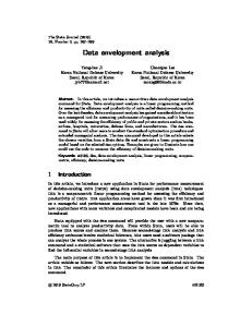
vided by the slack variables in the optimization, as they indicate the extend to which each input can be reduced to achieve an efficiency score of one (Choi/Murthi (2001), Kuosmanen/Cherchye/Sipiläinen (2006)). Thus, DEA not only measures efficiency, but can provide guidance as to how to improve the efficiency of inefficient funds. The left part of Figure 1 clarifies the principle of DEA with constant returns to scale in the case where one input is used for the production of one output. DEA with constant returns to scale

DEA with variable returns to scale

output

output

B

2

1

A

2

A

C

1

B

decreasing returns to scale

C

constant returns to scale

increasing returns to scale 0

Fig. 1

1

2

input

0

1

2

input

DEA with constant and variable returns to scale. This figure shows the DEA efficient frontier

with constant returns to scale (left) and with variable returns to scale (right) in the case where one input is used for the production of one output.

The straight line ascending from the origin in the left part of Figure 1 is called the efficient frontier. The points A, B, and C represent observed input-output combinations of different funds. Funds A and B exhibit the best input-output combinations and thus determine the efficient frontier. Fund C does not work efficiently; the output it obtains could be achieved with a lower input fund A employs, and the inputs of fund C are sufficient to achieve the output of fund B. The case of fund C is a good illustration of the efficiency score calculation. The efficiency score results from the relationship of the inputs necessary for efficient production (which is 1 in this case) to the actually used inputs (2 in this case). In this case the efficiency score is 0.5. If size differences have an influence on fund efficiency, assuming constant returns to scale would lead to a blending of scale efficiency due to size differences and technical efficiency. Employing an additional variable ci, the Banker/Charnes/Cooper (1984) approach introduces variable returns to scale:

8

R

Maximize ur

∑ u r yri +ci , subject to r=1

J

∑ v jx ji =1, j=1

R

J

r=1

j=1

∑ u r yri -∑ v jx ji -ci ≤ 0, u r ≥ 0, v j ≥ 0. (4)

The addition of variable returns to scale is the only difference between this model and that of Charnes/Cooper/Rhodes (1978). The right part of Figure 1 shows the principle of DEA with variable returns to scale, again using one input and one output factor. Assuming variable returns to scale, the efficient frontier ascending from the origin in the figure runs piecewise linear. Three ranges can be distinguished within the efficient frontier—increasing (ci < 0), constant (ci = 0), and decreasing (ci > 0) returns to scale. With increasing (decreasing) returns to scale, an increase of input leads to a disproportionately high (low) increase of output. With constant returns to scale, the increase of an input corresponds to the increase of an output. The approach of super efficiency presented by Andersen/Petersen (1993) is similar to the Banker/Charnes/Cooper (1984) approach. However, in the optimization, the fund under consideration is excluded from the calculation of the constraints. Therefore, efficient funds can attain an efficiency score larger than 1. This procedure makes a ranking of efficient funds possible. For inefficient funds, the efficiency score measured by the Andersen/Petersen (1993) model corresponds to the value calculated by the Banker/Charnes/Cooper (1984) model. Application of DEA models to hedge funds Regarding the application of DEA for hedge fund performance measurement, we first discuss the use of constant and variable returns to scale. Especially with hedge funds, the optimal fund size is an important problem against the background of different scale effects moving in opposite directions. On the one hand, hedge funds need a certain minimum capital to implement their strategies. For example, with the fixed-income arbitrage strategy very small market inefficiencies can be profitably exploited only if a large amount of capital is available. Moreover, fixed-cost degression results in larger funds working more efficiently. These two

9

effects indicate that hedge funds involve scale advantages and increasing returns to scale. On the other hand, hedge funds that are too large experience scale disadvantages. First, large hedge funds can create the risk that the funds will affect market prices by their own trading actions. This is particularly problematic with illiquid securities, because it is possible that closing the position will not be feasible at fair market prices. Second, finding profitable investment opportunities becomes more difficult with increasing fund size, a situation particularly true for funds specialized in a very close market segment. Thus, hedge funds also are subject to scale disadvantages and decreasing returns to scale. It is unknown how the scale advantages and disadvantages work in sum. The above discussion implies, however, that small funds may obtain increasing returns to scale at first, but that after attaining a certain size, become subject to decreasing returns to scale. Therefore, assuming variable returns to scale seems appropriate in applying DEA to hedge funds, which is in accordance with empirical evidence3 and the procedures employed by Gregoriou (2003), Wilkens/Zhu (2005), and Gregoriou/Sedzro/Zhu (2005). Nevertheless, DEA applications to traditional mutual funds usually use constant returns to scale (Murthi/Choi/Desai (1997), p. 411, Basso/Funari (2001), p. 481), even though most of the scale effects discussed with respect to hedge funds also affect traditional mutual funds.4 In order to evaluate the impact of model selection, we include applications with constant and with variable returns to scale in our empirical analysis.

3

4

Ammann/Moerth (2005) find a negative relationship between fund sizes and returns, but they also show that very small funds underperform on average. The underperformance of very small funds is explained by their higher total expense ratios. A negative relationship between standard deviations and fund sizes is also observed. Thus, we conclude that both risk and return are subject to variable returns to scale with hedge funds. Attributing the underperformance of very small funds to higher total expense ratios indicates that fund costs are also subject to variable returns to scale, which is in line with our discussion. Therefore, we conclude that costs are also subject to variable returns to scale with hedge funds. For example, Ferris/Chance (1987) find a negative relationship between the expense ratio and the size of mutual funds.

10

2.2 Systematization of Inputs and Outputs The selection of input and output factors is of high importance when using DEA. A basic result of the capital market theory is that there exists a functional relationship between risk and return of an investment—higher risk taking is rewarded with a higher return. Thus, in principle, risk measures are thought of as inputs, while return measures are interpreted as outputs. However, Nguyen-Thi-Thanh (2006) argues that some investors might be more concerned with central tendencies (mean, standard deviation), while others may care more about extreme values (skewness, kurtosis). Moreover, McMullen/Strong (1998) show that investors are concerned about risk and return over various time-horizons, as this provides more information than the performance of a single period only. Basso/Funari (2001) suggest that some investors may also include ethical criteria in decision making, and Murthi/Choi/Desai (1997) report that investors are interested in transaction costs. In the hedge fund context, it might also be important to consider hedge-fund-specific characteristics such as the minimum investment or the lock-up period (Nguyen-Thi-Thanh (2006)). Therefore, the selection of input and output variables is a complex task as the decision-maker is confronted with a large number of different attributes that might be of differing importance. However, by the choice of inputs and outputs and by setting additional constraints in the optimization, DEA is able to include all the investor’s financial, risk-aversion, diversification, and investment horizon constraints. Consequently, DEA can be a tailor-made decision-making tool that exactly suits the investor’s preferences (Nguyen-Thi-Thanh (2006)). In this section possible inputs and outputs for DEA are presented, systematized, and discussed with respect to their suitability for hedge fund performance measurement. Table

2

shows

the

inputs

and

outputs

suggested

in

Gregoriou

(2003),

Gregoriou/Sedzro/Zhu (2005), Wilkens/Zhu (2005), and Nguyen-Thi-Thanh (2006).

11

TABLE 2 Inputs and outputs considered in the literature category inputs

outputs

Gregoriou (2003), Gregoriou/Sedzro/Zhu (2005) lower partial moments of order 1 lower partial moments of order 2 lower partial moments of order 3 higher partial moments of order 1 higher partial moments of order 2 higher partial moments of order 3

Wilkens/Zhu (2005)

Nguyen-Thi-Thanh (2006)

standard deviation lower partial moments of order 0

standard deviation excess kurtosis

average return skewness minimum return

average return skewness

This table shows the inputs and outputs used in the four papers that applied DEA to measure the performance of hedge funds. Gregoriou (2003) and Gregoriou/Sedzro/Zhu (2005) choose lower and higher partial moments; Wilkens/Zhu (2005) and Nguyen-Thi-Thanh (2006) also include the average return, the standard deviation of returns, and the higher moments of the return distribution in the DEA of hedge funds.

To capture the tail characteristics of hedge fund returns Gregoriou (2003) and Gregoriou/ Sedzro/Zhu (2005) use the lower partial moments (LPM) of order 1 to 3 as inputs and the higher partial moments (HPM) of order 1 to 3 as outputs. Wilkens/Zhu (2005) choose some measures often employed in hedge fund analysis. They consider the standard deviation and the portion of negative returns (which is the lower partial moment of order 0) as inputs and the average return, the skewness, and the minimum return as outputs. Because investors might have positive preferences for odd moments and negative preferences for even moments Nguyen-Thi-Thanh (2006) chooses standard deviation and excess kurtosis as inputs and average return and skewness as outputs. It seems fair to conclude from the literature that there is no agreement as to which measures should be used as inputs and outputs for a DEA-based performance measurement of hedge funds.5 Table 3 sets out a selection of the most common risk, return, and cost measures that might be regarded as inputs and outputs in DEA. The measures presented do not necessarily comprise a complete list of all possible risk, return, and cost measures, as individual investors might consider other measures as relevant.

5

The difficulty in selecting inputs and outputs applies not only to hedge funds, but more so to banks. For a discussion of inputs and outputs of banks see Bessler/Norsworthy (2005).

12

TABLE 3 Possible inputs and outputs Inputs risk measures

higher moments cost measures outputs return measures

higher moments

standard deviation (SD) lower partial moments of order 0 (LPM0) lower partial moments of order 1 (LPM1) lower partial moments of order 2 (LPM2) lower partial moments of order 3 (LPM3) maximum drawdown (MD) average drawdown (AD) standard deviation of drawdown (SDD) value at risk (VAR) conditional value at risk (CVAR) modified value at risk (MVAR) beta factor residual volatility tracking error excess kurtosis loads, fees trading activity arithmetic excess return (AER) geometric excess return (GER) higher partial moment of order 0 (HPM0) higher partial moment of order 1 (HPM1) higher partial moment of order 2 (HPM2) higher partial moment of order 3 (HPM3) Skewness

total risk

downside risk

included in the empirical part

systematic risk unsystematic risk

not included in the empirical part

included in the empirical part not included in the empirical part

This table shows a selection of the most common risk, return, and cost measures that might be regarded as inputs and outputs in DEA. Inputs include risk measures, cost measures, and higher moments. Outputs include return measures and higher moments. Eleven inputs and six outputs will be used in the empirical section of this paper. The formulas for calculating the measures included in the empirical investigation can be found in Appendix A.

There is a wide variety of classic and newer risk measures that can be included as inputs. The standard deviation measures the total risk of an investment, which gives both the positive and negative deviations of the returns from the expected value. However, this is not the general understanding of risk. In contrast, LPMs only consider negative deviations of returns from a minimal acceptable return, a situation that most investors view with disfavor. Thus, LPMs might seem a more appropriate measure of risk. The choice of order n determines the extent to which the deviation from the minimal acceptable return is weighted. The drawdown of a fund is the loss incurred over a given investment period. The three drawdown-based risk measures listed in Table 3 are defined as the largest possible loss (the so-called maximum drawdown), an average of the largest drawdowns, or a type of standard deviation of the largest drawdowns.

13

Value at risk describes the possible loss of an investment, which is not exceeded with a given probability of 1-α in a certain period. To take into account the distribution of returns below the value at risk, the literature frequently considers expected loss under the condition that the value at risk is exceeded (Artzner et al. (1999)). This leads to the conditional value at risk. To include skewness and excess kurtosis in computing value at risk, the Cornish-Fisher expansion can be used, which leads to the modified value at risk (Gregoriou/Gueyie (2003)). Measures for systematic (beta factor) and unsystematic risk (residual volatility and tracking error) could be integrated into DEA. But these measures are less suitable for performance measurement of hedge funds in our context because they require the definition of a benchmark. Usually, hedge funds attempt to achieve positive returns independent of any market index and therefore the definition of a standardized benchmark is neither possible nor meaningful. Therefore, these risk measures are excluded from the empirical investigation.6 The cost measures that are used as inputs in conducting DEA for mutual funds are likewise less suitable for performance measurement of hedge funds, as front-end loads, administration, and management fees are already contained in the fund returns (all hedge fund returns are net of fees). It is important to note that one could argue that even if returns are net of all fees, fee consideration can still provide additional information about the fund manager’s performance because there is a difference between a fund that has a gross return of 10% and a net return of 5%, and a fund that has a gross return of 20% and a net return of 5% (Choi/Murthi (2001)). But even if information on returns before fees was available, a comparison of hedge funds on the basis of cost measures would not be meaningful due to the complexity and heterogeneity of the fee structure (Le

6

From a theoretical point of view, the beta factor is not suited if the performance of hedge funds is evaluated in isolation but it is the right measure if the investor only wants to add a small percentage of hedge funds to his existing investment portfolio. See Scholz/Wilkens (2003) for a related discussion. Therefore it would be necessary to measure the systematic risk contribution of the fund under evaluation in relation to the investor’s portfolio. As this goes far beyond the scope of this contribution, we restrict ourselves to the evaluation of hedge funds in isolation and exclude this portfolio theoretical investigation. However, in Appendix B we show that our main results are robust for an evaluation from the portfolio perspective. For this purpose, we measure the performance of a portfolio of traditional investments and a small portion of hedge funds (1%, 5%, and 10%). Detailed results are available upon request.

14

Moigne/Savaria (2006)). An example is the individual high watermark. Thus, standardized comparisons as used in evaluating mutual funds, e.g., with front-end loads, are not possible for hedge funds. The same is true for trading-activity-based measures, also included in mutual fund DEA. Because hedge fund managers do not publish their trading activity, there is no data available to make such a comparison between different hedge funds. Compared to the input side, the number of possible return measures on the output side is small. In most of the literature, only excess return is used as an output, making it necessary merely to decide whether the average return should be computed arithmetically or geometrically. The arithmetic case assumes withdrawal of gains; the geometric case assumes reinvestment of gains. Gregoriou (2003) and Gregoriou/Sedzro/Zhu (2005) also use a counterpart of the LPMs as return measure, that is, the higher partial moments (HPM). As mentioned, Wilkens/Zhu (2005) and Nguyen-Thi-Thanh (2006) use skewness and kurtosis in DEA as inputs and outputs. Similar to hedge fund costs, we will not integrate skewness or kurtosis in DEA because these characteristics are already displayed by many risk measures on the input side. Skewness and kurtosis, for example, explicitly enter the computation of the modified value at risk so that additional consideration of the higher moments is not necessary in our framework. 2.3 Input and Output Selection Rules The question now arise which and how many of these input and output measures should be used for a DEA of hedge funds. Counterintuitively, using too many inputs and outputs will be less helpful because when the number of inputs and outputs increases, more decision-making units tend to get an efficiency score of 1 as they become too specialized to be evaluated with respect to other units.7 A rule of thumb is that there should be a minimum of three funds per input and output in implementing a DEA model (Bowlin 7

Problems related to discrimination and model misspecification arise when there are a relatively large number of variables compared to the number of funds, which may cause the majority of funds to be defined as efficient. Thus, the inclusion of more inputs and outputs in the model can artificially inflate the efficiency scores as the addition of each variable provides an additional dimension in which the

15

(1998), p. 18). Thus, for practical reasons, there needs to be some limit on the number of inputs and outputs. As mentioned, to date there has been no agreement or rule for the selection of inputs and outputs. From an economic point of view, the input and output selection should be based on the investor’s preferences because different investors might consider different measures as relevant. The correct approach would thus be to evaluate the distribution function of the returns of a particular hedge fund by using the investor’s utility function.8 The problem with this procedure is that hedge fund performance is often reported in a multitude of separate measures, as single measures cannot account for the full complexity of hedge fund returns. The investor is confronted with a large number of possible measures, any or all of which might be of particular relevance. We recommend tackling this problem by using DEA, which is capable of integrating the complexity of hedge fund returns into performance measurement. For this purpose, those inputs and outputs should be selected that differ as much as possible from each other in order to reach the highest possible explanatory power in performance measurement.9 We propose two selection rules that meet this criterion. The first is based on Spearman’s rank correlation; the second on principal component analysis.10 Selection rule based on Spearman’s rank correlation The selection rule based on Spearman (1904) consists of selecting those inputs and outputs that are correlated as little as possible. Here the selection of inputs and outputs is a

8

9

10

model will seek similar comparison peers. See Pedraja-Chaparro/Salinas-Jimenez/Smith (1999) and Adler/Golany (2002). There are different ways to integrate investor’s preferences into DEA. See Allen et al. (1997) and Halme et al. (1999). A simple example would be a scoring approach similar to the proposed selection rule based on principal components; the only difference is that the input and output weights are not determined by an optimization but are estimated by the investor. If the investor already knows which measures are relevant and if he knows the relative importance of each of these measures, there is no further selection rule necessary. Thus, the selection rules presented in the following are helpful (1) for those investors who cannot decide between the large number of possible measures, (2) for those investors who have chosen too many inputs and outputs, and (3) for those investors who cannot identify the relative importance of the inputs and outputs chosen. The main motivation for the proposed selection rules is that they are helpful in achieving a high-quality DEA model. The DEA model could be misspecified if relevant factors are omitted or if irrelevant factors are included (Smith (1997)). For example, an input that has a correlation of 1 to another input might be considered irrelevant for the DEA analysis, as it cannot provide any new information

16

three-step procedure: In the first step, all risk and return measures are computed for all funds. In the second step, the measurement values are ranked so as to determine an order of the funds. In the third step, this ranking is used to determine the rank correlation between the measures; those measures with the smallest rank correlations are selected as inputs and outputs. The selection rule based on Spearman’s rank correlation coefficient (rsp) is stated formally for the inputs as: I ⎛ ⎞ arg min rsp j1,j2 = 1 − ⎜ 6 ⋅ ∑ d i2 ⎟ 1≤ j1,j2≤ J ⎝ i =1 ⎠

(I

3

− I) ,

(5)

− I) ,

(6)

and for the outputs as: I ⎛ ⎞ arg min rsp r1,r2 = 1 − ⎜ 6 ⋅ ∑ d i2 ⎟ 1≤ r1,r2≤ R ⎝ i =1 ⎠

(I

3

with di as differences in ranking places for fund i. Under this selection rule, two inputs and two outputs are selected, which are those with the smallest rank correlation. (for more details on rank correlation analysis see Kendall/Gibbons (1990)). Selection rule based on principal component analysis Principal component analysis is a variable reduction procedure. It extracts the most important information by building a number of artificial variables that account for most of the variance in the observed variables. These artificial variables are called principal components. According to the second selection rule, the principal components should be used in DEA to integrate the variability of all risk and return measures (Adler/Golany (2002)). Technically, a principal component is a linear combination of optimallyweighted observed variables. Starting with the observed variables X1 to XN, principal component analysis provides the following linear system of equations: CA = γ1A · X1 + γ2A · X2 … + γNA · XN, CB = γ1B · X1 + γ2B · X2 … + γNB · XN,…

(7)

(Pedraja-Chaparro/Salinas-Jimenez/Smith (1999)). The presented selection rules avoid these problems by distinguishing relevant from irrelevant factors and thus improve the model quality.

17

The first principal component CA is the result of a linear combination of the observed variables X1 to XN with the factor loadings γ1A to γNA. In the optimization, the factor loadings are weighted so as to maximize the portion of variance explained by the principal components. The eigenvector with the largest eigenvalue determines the first principal component, while the eigenvector with the second largest eigenvalue determines the second principal component (for more details on principal component analysis see Jackson (2003) and Jolliffe (2002)). The practical implementation of both selection rules is shown in the following section.

3 EMPIRICAL INVESTIGATION 3.1 Data and Procedure In the empirical investigation we consider monthly returns for 30 hedge funds between January 1996 and December 2005. The hedge funds were selected from the Center for International Securities and Derivatives Markets (CISDM) hedge fund database.11 To obtain a representative sample of the entire hedge fund universe, we randomly choose two funds from each of the 15 strategy groups included in the database.12 The performance of these 30 funds is evaluated by ten DEA applications. The results of the applications are compared both among themselves and with classic performance measures. Table 4 gives an overview of the ten applications.

11 12

The CISDM hedge fund database has been subject of many academic studies. For the properties of this database, see, e.g., Edwards/Caglayan (2001), Kouwenberg (2003), Capocci/Hübner (2004). Altogether we analyzed 450 hedge funds. We repeated the investigation 15 times with 30 funds from each of the strategy groups and found that our main results are robust with regard to these variations. We also found robust results regarding different time-horizons. The results of all robustness tests are presented in Appendix B. Detailed results are available upon request.

18

TABLE 4 Overview of the applications Application 1 2 3 4

input standard deviation standard deviation LPM1,LPM2, LPM3 standard deviation, LPM0

Output excess return excess return HPM1, HPM2, HPM3 average return, skewness, minimum return

returns to scale constant variable variable variable

5 6 7 8 9 10

constant selection rule based on selection rule based on variable Spearman’s rank correlation Spearman’s rank correlation variable constant selection rule based on selection rule based on variable principal component analysis principal component analysis variable

underlying modeling approach Charnes/Cooper/Rhodes (1978) Banker/Charnes/Cooper (1984) Banker/Charnes/Cooper (1984) Banker/Charnes/Cooper (1984) Charnes/Cooper/Rhodes (1978) Banker/Charnes/Cooper (1984) Andersen/Petersen (1993) Charnes/Cooper/Rhodes (1978) Banker/Charnes/Cooper (1984) Andersen/Petersen (1993)

This table shows the inputs, outputs, returns to scale assumption, and underlying modeling approach for the 10 DEA applications considered in the empirical investigation. Applications 1 to 4 are already covered in the literature. Applications 5 to 10 extend the literature by choosing inputs and outputs following the selection rules presented in Section 2.3. The selection of inputs and outputs is based on Spearman’s rank correlation for Applications 5 to 7 and on principal component analysis for Applications 8 to 10. The abbreviations are explained in Table 3.

Application 1 clarifies the connection between classic performance measurement and DEA. Its input is standard deviation and its output is excess return. Assuming constant returns to scale, Application 1 results in the same ranking and evaluation of the investments as is made by the Sharpe ratio (SRi), calculated as the arithmetic excess return divided by the standard deviation). In Application 2, the assumption of constant returns to scale is replaced by variable returns to scale. Applications 3 to 10 use a multi-dimensional performance measurement instead of a two-dimensional approach. Application 3 is the one presented by Gregoriou (2003) and Gregoriou/Sedzro/Zhu (2005). Application 4 was analyzed by Wilkens/Zhu (2005). Applications 5 to 10 extend the literature by choosing inputs and outputs following the selection rules presented in Section 2.3. Applications 5 to 7 use the selection rule based on Spearman’s rank correlation, but use various underlying DEA models: Application 5 is based on Charnes/Cooper/Rhodes (1978), Application 6 on Banker/Charnes/Cooper (1984), and Application 7 on Andersen/Petersen (1993). Applications 8 to 10 use the selection rule based on principal component analysis. Again, these applications differ with respect to the underlying DEA model. Various comparisons between the applications are possible and meaningful. The results of the classic Sharpe ratio can be compared with the results of the DEA analysis. Appli-

19

cation 1 and 2 allow a direct comparison of the Charnes/Cooper/Rhodes (1978) and Banker/Charnes/Cooper (1984) models. This clarifies the influence of variable economies of scale on fund efficiency. Moreover, applications already proposed in the literature (Application 3 and 4) can be contrasted with applications using the new selection rules (Applications 5 to 10). Section 3.2 presents the selection of inputs and outputs. Then, in Section 3.3, DEA performance measurement is performed. To solve the DEA optimization problem, the EMS (efficiency measurement system) software presented by Scheel (2000) is employed. 3.2 Selection of Inputs and Outputs Selection rule based on Spearman’s rank correlation Following the selection rule based on Spearman’s rank correlation, we first calculate all measures for the 30 funds. A constant risk-free interest rate of rf = 0.35% per month was used. This corresponds to the interest on 10-year U.S. treasury bonds as of December 30, 2005 (4.28% per annum). For the LPM-based measures, the minimal acceptable return corresponds to the risk-free monthly interest rate (τ = 0.35%). For the average drawdown and the standard deviation of drawdown, the five largest drawdowns are considered (K = 5). The value-at-risk-based performance measures were calculated using a significance level of α = 0.05. The results for the inputs are presented in Table 5 (panel A). In the parentheses the measurement values are ranked in order to determine the rank correlation in the next step. The rankings presented in panel A of Table 5 illustrate the complexity of hedge fund performance measurement. For example, Fund 27 has the highest standard deviation, but it ranks at 10th place with the modified value at risk. Fund 24 is in second place with the standard deviation, but at 21st place with the modified value at risk. These results confirm the significance of a multi-dimensional approach when assessing hedge fund performance and thus emphasize the benefit of DEA in performance measurement.

20

TABLE 5 Measurement value and ranking of inputs Panel A: Measurement value and ranking (in parentheses) of inputs input SD LPM0 LPM1 LPM2 LPM3 MD fund 1 1.50 (26) 28.33 (29) 0.37 (23) 0.01 (21) 0.00 (20) 8.52 (23) 2 1.29 (27) 34.17 (22) 0.35 (24) 0.01 (24) 0.00 (25) 9.34 (22) 3 1.63 (23) 34.78 (21) 0.34 (25) 0.00 (27) 0.00 (27) 6.16 (26) 4 0.98 (29) 46.27 (5) 0.32 (27) 0.00 (29) 0.00 (29) 3.23 (29) 5 3.89 (10) 36.21 (19) 0.94 (10) 0.07 (8) 0.01 (7) 22.85 (11) 6 4.71 (8) 37.38 (17) 1.30 (8) 0.11 (6) 0.02 (2) 46.84 (2) 7 6.92 (3) 51.28 (3) 1.53 (6) 0.15 (2) 0.03 (1) 48.71 (1) 8 5.68 (5) 41.18 (15) 1.70 (4) 0.13 (5) 0.02 (4) 32.10 (6) 9 2.86 (13) 33.33 (23) 0.72 (14) 0.02 (15) 0.00 (15) 18.83 (14) 10 5.22 (7) 40.83 (16) 1.73 (3) 0.13 (4) 0.01 (6) 38.77 (4) 11 6.83 (4) 42.37 (13) 1.93 (1) 0.15 (1) 0.02 (3) 19.93 (13) 12 2.81 (14) 33.33 (23) 0.79 (12) 0.04 (13) 0.00 (13) 18.37 (15) 13 1.71 (22) 44.17 (8) 0.52 (18) 0.01 (20) 0.00 (21) 5.99 (27) 14 2.96 (12) 52.50 (2) 1.20 (9) 0.05 (10) 0.00 (12) 43.14 (3) 15 0.99 (28) 35.83 (20) 0.27 (29) 0.01 (25) 0.00 (23) 11.79 (20) 16 2.36 (20) 41.67 (14) 0.65 (15) 0.02 (17) 0.00 (17) 12.02 (19) 17 2.56 (15) 33.33 (23) 0.41 (21) 0.04 (12) 0.01 (8) 24.97 (9) 18 1.61 (24) 30.67 (27) 0.28 (28) 0.00 (28) 0.00 (28) 4.80 (28) 19 2.44 (19) 43.48 (10) 0.57 (16) 0.02 (18) 0.00 (16) 14.14 (17) 20 2.54 (18) 20.83 (30) 0.50 (19) 0.04 (11) 0.01 (10) 30.75 (7) 21 2.56 (16) 32.00 (26) 0.34 (26) 0.01 (23) 0.00 (24) 6.59 (24) 22 0.88 (30) 29.17 (28) 0.12 (30) 0.00 (30) 0.00 (30) 2.42 (30) 23 3.07 (11) 42.50 (12) 0.77 (13) 0.02 (16) 0.00 (18) 23.08 (10) 24 7.21 (2) 49.23 (4) 0.82 (11) 0.03 (14) 0.00 (14) 16.30 (16) 25 1.57 (25) 44.17 (8) 0.38 (22) 0.01 (26) 0.00 (26) 6.32 (25) 26 5.53 (6) 42.59 (11) 1.66 (5) 0.10 (7) 0.01 (9) 22.12 (12) 27 7.80 (1) 45.00 (6) 1.78 (2) 0.13 (3) 0.01 (5) 35.12 (5) 28 3.89 (9) 45.00 (6) 1.30 (7) 0.06 (9) 0.00 (11) 26.82 (8) 29 1.81 (21) 53.57 (1) 0.48 (20) 0.01 (22) 0.00 (22) 12.79 (18) 30 2.55 (17) 36.67 (18) 0.52 (17) 0.01 (19) 0.00 (19) 10.71 (21) Panel B: Rank correlation of inputs SD 1.00 0.38 0.92 0.91 0.87 0.81 LPM0 0.38 1.00 0.46 0.29 0.24 0.28 LPM1 0.92 0.46 1.00 0.94 0.89 0.81 LPM2 0.91 0.29 0.94 1.00 0.98 0.90 LPM3 0.87 0.24 0.89 0.98 1.00 0.91 MD 0.81 0.28 0.81 0.90 0.91 1.00 AD 0.90 0.33 0.95 0.96 0.93 0.87 SDD 0.87 0.32 0.91 0.96 0.95 0.96 VAR 0.99 0.41 0.93 0.94 0.91 0.85 CVAR 0.86 0.23 0.83 0.95 0.97 0.90 MVAR 0.77 0.30 0.88 0.93 0.93 0.88

AD 5.51 4.90 2.73 1.88 12.25 14.20 16.83 18.13 7.91 12.79 18.18 8.59 4.65 12.36 3.67 6.84 5.52 1.83 5.97 8.67 3.07 1.04 8.65 8.90 3.32 16.76 22.91 13.64 3.06 6.24 0.90 0.33 0.95 0.96 0.93 0.87 1.00 0.96 0.93 0.87 0.89

SDD (20) (21) (27) (28) (10) (6) (4) (3) (15) (8) (2) (14) (22) (9) (23) (16) (19) (29) (18) (12) (25) (30) (13) (11) (24) (5) (1) (7) (26) (17)

12.95 13.52 7.62 4.63 30.55 48.75 52.48 47.62 21.76 40.84 40.77 24.64 10.67 44.42 12.28 16.39 25.06 5.72 18.01 31.43 8.32 2.89 26.68 23.85 8.46 38.13 53.15 35.29 12.87 16.23 0.87 0.32 0.91 0.96 0.95 0.96 0.96 1.00 0.91 0.91 0.92

(21) (20) (27) (29) (11) (3) (2) (4) (16) (6) (7) (14) (24) (5) (23) (18) (13) (28) (17) (10) (26) (30) (12) (15) (25) (8) (1) (9) (22) (19)

VAR

CVAR

1.66 (26) 1.49 (27) 1.78 (24) 1.09 (29) 5.03 (10) 6.91 (8) 10.64 (2) 7.94 (5) 3.48 (15) 7.88 (6) 9.48 (4) 3.64 (14) 2.20 (22) 4.66 (11) 1.16 (28) 3.17 (19) 3.77 (13) 1.70 (25) 3.26 (17) 3.32 (16) 3.06 (20) 0.67 (30) 3.97 (12) 10.01 (3) 1.92 (23) 7.80 (7) 10.73 (1) 5.59 (9) 2.57 (21) 3.21 (18)

2.98 2.27 2.25 1.44 8.90 13.14 15.94 11.64 4.35 11.46 13.20 6.38 3.14 6.76 3.01 4.88 21.53 2.63 5.35 9.46 3.57 1.63 4.36 7.40 2.77 8.98 14.60 7.77 3.73 4.23

0.99 0.41 0.93 0.94 0.91 0.85 0.93 0.91 1.00 0.91 0.82

0.86 0.23 0.83 0.95 0.97 0.90 0.87 0.91 0.91 1.00 0.86

MVAR (24) (27) (28) (30) (10) (5) (2) (6) (18) (7) (4) (14) (22) (13) (23) (16) (1) (26) (15) (8) (21) (29) (17) (12) (25) (9) (3) (11) (20) (19)

1.94 1.58 1.24 1.05 6.09 7.79 11.43 8.32 3.46 8.13 9.43 4.23 2.05 4.88 1.52 2.81 3.48 0.86 3.12 4.28 -2.12 0.36 2.87 1.64 1.27 7.64 4.85 5.58 2.46 0.44 0.77 0.30 0.88 0.93 0.93 0.88 0.89 0.92 0.82 0.86 1.00

Panel A of this table shows, for each of the 30 funds, the measurement results for the 11 inputs defined in Section 2.2. The numbers in parentheses indicate the ranking of the measurement values. Panel B shows the resulting Spearman’s rank correlation between the inputs. The abbreviations are explained in Table 3. The formulas for calculation of the measures can be found in Appendix A.

Using the ranking shown in Table 5, the rank correlation between the measures is derived, as set out in panel B of Table 5. The measures that exhibit the smallest rank correlations are selected as inputs and outputs. We find the minimum rank correlation comparing conditional value at risk and lower partial moment of order 0. The rank correlation here is 0.23.

(20) (22) (25) (26) (7) (5) (1) (3) (14) (4) (2) (12) (19) (9) (23) (17) (13) (27) (15) (11) (30) (29) (16) (21) (24) (6) (10) (8) (18) (28)

21

The measurement values and rankings for the outputs are presented in Table 6. The minimum rank correlation is found with the higher partial moment of order 3 and higher partial moment of order 0. The rank correlation here is –0.33. TABLE 6 Measurement value and ranking of outputs Panel A: Measurement value and ranking (in parentheses) of outputs input fund AER GER HPM0 1 0.45 (17) 0.44 (13) 71.67 (2) 2 0.29 (24) 0.28 (19) 65.83 (9) 3 0.55 (13) 0.16 (24) 65.22 (10) 4 0.17 (26) -0.06 (28) 53.73 (26) 5 1.02 (5) 0.90 (3) 63.79 (12) 6 0.48 (15) 0.29 (18) 62.62 (14) 7 0.39 (20) -0.03 (26) 48.72 (28) 8 1.06 (4) 0.89 (4) 58.82 (16) 9 0.87 (7) 0.83 (5) 66.67 (6) 10 0.35 (22) 0.21 (22) 59.17 (15) 11 1.40 (3) 1.15 (2) 57.63 (18) 12 0.64 (10) 0.60 (8) 66.67 (6) 13 0.25 (25) 0.24 (20) 55.83 (22) 14 -0.14 (30) -0.18 (30) 47.50 (29) 15 0.12 (27) 0.12 (25) 64.17 (11) 16 0.36 (21) 0.33 (16) 58.33 (17) 17 0.10 (28) -0.04 (27) 66.67 (6) 18 0.59 (12) 0.23 (21) 69.33 (4) 19 0.41 (19) 0.21 (23) 56.52 (21) 20 0.51 (14) 0.47 (12) 79.17 (1) 21 0.80 (8) 0.58 (10) 68.00 (5) 22 0.42 (18) 0.42 (14) 70.83 (3) 23 0.73 (9) 0.68 (6) 57.50 (19) 24 1.50 (2) 0.53 (11) 50.77 (27) 25 0.31 (23) 0.30 (17) 55.83 (22) 26 0.94 (6) 0.68 (7) 57.41 (20) 27 1.75 (1) 1.48 (1) 55.00 (24) 28 0.46 (16) 0.38 (15) 55.00 (24) 29 0.05 (29) -0.17 (29) 46.43 (30) 30 0.63 (11) 0.60 (9) 63.33 (13) Panel B: Rank correlation of outputs AER 0.88 0.17 1.00 GER 0.88 1.00 0.24 HPM0 0.17 0.24 1.00 HPM1 0.68 0.69 -0.19 HPM2 0.72 0.64 -0.30 0.71 0.59 -0.33 HPM3

HPM1 0.83 0.64 0.51 0.26 1.92 1.69 1.66 2.75 1.59 2.08 3.30 1.43 0.77 1.06 0.40 1.01 0.40 0.52 0.80 1.00 0.94 0.54 1.50 1.47 0.69 2.48 3.53 1.76 0.32 1.15 0.68 0.69 -0.19 1.00 0.96 0.90

(19) (23) (26) (30) (6) (8) (9) (3) (10) (5) (2) (13) (21) (15) (27) (16) (28) (25) (20) (17) (18) (24) (11) (12) (22) (4) (1) (7) (29) (14)

HPM2 0.01 0.01 0.01 0.00 0.09 0.09 0.15 0.20 0.06 0.14 0.32 0.05 0.02 0.04 0.00 0.04 0.01 0.02 0.03 0.02 0.05 0.01 0.08 0.26 0.02 0.18 0.50 0.09 0.01 0.06 0.72 0.64 -0.30 0.96 1.00 0.98

(23) (25) (24) (30) (10) (8) (6) (4) (12) (7) (2) (15) (21) (16) (29) (17) (28) (22) (18) (19) (14) (26) (11) (3) (20) (5) (1) (9) (27) (13)

HPM3 0.00 0.00 0.00 0.00 0.00 0.01 0.02 0.02 0.00 0.01 0.04 0.00 0.00 0.00 0.00 0.00 0.00 0.00 0.00 0.00 0.01 0.00 0.01 0.07 0.00 0.02 0.13 0.01 0.00 0.01

(24) (26) (23) (29) (13) (8) (5) (4) (14) (7) (3) (16) (22) (17) (30) (15) (27) (20) (18) (21) (9) (28) (11) (2) (19) (6) (1) (10) (25) (12)

0.71 0.59 -0.33 0.90 0.98 1.00

Panel A of this table shows, for each of the 30 funds, the measurement results for the six outputs defined in Section 2.2. The numbers in parentheses indicate the ranking of the measurement values. Panel B shows the resulting Spearman’s rank correlation between the outputs. The abbreviations are explained in Table 3. The formulas for calculation of the measures can be found in Appendix A.

Thus, in Applications 5 to 7 the conditional value at risk and the lower partial moment of order 0 will be used as inputs and the higher partial moment of order 3 and of order 0 will be used as outputs.

22

Selection rule based on principal component analysis Principal components are calculated using SPSS. The results obtained for the inputs and outputs are shown in Table 7. TABLE 7 Results of principal component analysis inputs standard deviation LPM0 LPM1 LPM2 LPM3 maximum drawdown average drawdown standard dev. of drawdown value at risk conditional value at risk modified value at risk total variance explained (%)

component A 0.90 0.45 0.95 0.97 0.91 0.87 0.96 0.97 0.93 0.82 0.91 78.94

component B -0.05 0.86 0.20 -0.06 -0.27 -0.05 0.16 0.05 -0.05 -0.36 -0.04 88.20

outputs arithmetic excess return geometric excess return HPM0 HPM1 HPM2 HPM3

component A 0.94 0.89 0.11 0.90 0.95 0.86

component B 0.01 0.39 0.97 0.07 -0.24 -0.34

total variance explained (%)

69.11

90.15

The left side of this table shows the principal component analysis results for the 11 inputs defined in Section 2.2. For each of the inputs, two factor loadings are calculated; the first one for component A and the second one for component B. The last row gives the total variance explained by the principal components. The right side of the table shows the corresponding results for the six outputs defined in Section 2.2. The abbreviations are explained in Table 3. The formulas for calculation of the measures can be found in Appendix A.

On the input side, the lower partial moment of order 2 has the highest impact on component A (factor loading 0.97), while the lower partial moment of order 0 is the most important factor for component B (factor loading 0.86). Components A and B together account for 88.20% of the variance in the input data. On the output side, the higher partial moment of order 2 (factor loading 0.95, component A) and the higher partial moment of order 0 (factor loading 0.97, component B) have the highest impact in the principal component analysis. Components A and B explain 90.15% of the total variance. Using the principal component analysis results, we calculate inputs and outputs for Applications 8 to 10: On the input side, the first principal component is the result of a linear combination of the observed variables SD to MVAR with the factor loadings 0.90 to 0.91. The second principal component uses the factor loadings –0.05 to –0.04. On the output side, the first principal component combines the results of the observed variables AER to HPM3 with the factor loadings 0.94 to 0.86, while the second principal component has the loadings 0.01 to –0.34.

23

3.3 DEA Performance Measurement Table 8 (panel A) shows the performance measurement results for the classic Sharpe ratio and for the ten DEA applications. Furthermore, for each measure the resulting fund rankings are presented. The Spearman’s rank correlation coefficients between the performance measures are set out in panel B of Table 8 in order to illustrate the relations between the applications. TABLE 8 Performance measurement results Panel A: Performance measurement values and ranking (in parentheses) of funds fund Sharpe DEA Application ratio 1 2 3 4 5 6 1 0.30 (6) 0.63 (6) 0.68 (15) 0.74 (15) 0.68 (17) 0.97 (6) 0.98 (7) 2 0.22 (12) 0.46 (12) 0.68 (16) 0.49 (23) 0.68 (18) 0.78 (10) 0.80 (12) 3 0.34 (3) 0.71 (3) 0.88 (10) 0.51 (22) 0.88 (11) 0.50 (23) 0.96 (8) 4 0.18 (18) 0.37 (18) 0.90 (7) 0.70 (16) 1.00 (1) 0.43 (27) 0.77 (15) 5 0.26 (7) 0.55 (7) 0.95 (6) 0.93 (10) 0.97 (9) 0.59 (13) 0.62 (19) 6 0.10 (25) 0.21 (25) 0.24 (28) 0.58 (19) 0.33 (26) 0.75 (12) 0.82 (11) 7 0.06 (27) 0.12 (27) 0.13 (30) 0.48 (24) 0.25 (30) 0.37 (28) 0.63 (18) 8 0.19 (17) 0.39 (17) 0.69 (14) 0.79 (12) 0.70 (16) 0.55 (17) 0.57 (25) 9 0.31 (5) 0.64 (5) 1.00 (1) 1.00 (1) 1.00 (1) 0.77 (11) 0.79 (13) 10 0.07 (26) 0.14 (26) 0.17 (29) 0.56 (21) 0.29 (29) 0.52 (20) 0.55 (28) 11 0.21 (14) 0.43 (14) 0.86 (11) 0.86 (11) 0.86 (12) 0.56 (14) 0.59 (21) 12 0.23 (10) 0.47 (10) 0.64 (17) 0.78 (13) 0.64 (19) 0.54 (18) 0.61 (20) 13 0.15 (22) 0.31 (22) 0.51 (20) 0.47 (25) 0.51 (22) 0.51 (22) 0.58 (23) 14 -0.05 (30) 0.00 (30) 0.30 (26) 0.34 (28) 0.30 (28) 0.35 (29) 0.39 (30) 15 0.12 (23) 0.26 (23) 0.88 (9) 0.43 (27) 0.88 (10) 1.00 (1) 1.00 (1) 16 0.15 (21) 0.32 (21) 0.37 (23) 0.57 (20) 0.37 (25) 0.52 (21) 0.56 (27) 17 0.04 (28) 0.08 (28) 0.34 (25) 0.29 (29) 0.83 (13) 0.53 (19) 0.78 (14) 18 0.37 (2) 0.77 (2) 1.00 (1) 1.00 (1) 1.00 (1) 0.84 (8) 1.00 (1) 19 0.17 (20) 0.35 (20) 0.36 (24) 0.45 (26) 0.40 (24) 0.48 (25) 0.58 (24) 20 0.20 (15) 0.42 (15) 0.49 (21) 0.75 (14) 1.00 (1) 1.00 (1) 1.00 (1) 21 0.31 (4) 0.65 (4) 0.98 (5) 1.00 (1) 1.00 (1) 0.86 (7) 0.91 (9) 22 0.48 (1) 1.00 (1) 1.00 (1) 1.00 (1) 1.00 (1) 1.00 (1) 1.00 (1) 23 0.24 (9) 0.50 (9) 0.72 (12) 1.00 (1) 0.72 (14) 0.56 (15) 0.59 (22) 24 0.21 (13) 0.43 (13) 0.89 (8) 1.00 (1) 1.00 (1) 1.00 (1) 1.00 (1) 25 0.20 (16) 0.41 (16) 0.56 (19) 0.70 (17) 0.63 (20) 0.55 (16) 0.63 (17) 26 0.17 (19) 0.36 (19) 0.59 (18) 0.98 (8) 0.60 (21) 0.79 (9) 0.83 (10) 27 0.22 (11) 0.47 (11) 1.00 (1) 1.00 (1) 1.00 (1) 1.00 (1) 1.00 (1) 28 0.12 (24) 0.24 (24) 0.26 (27) 0.62 (18) 0.31 (27) 0.46 (26) 0.50 (29) 29 0.03 (29) 0.06 (29) 0.49 (22) 0.25 (30) 0.49 (23) 0.32 (30) 0.77 (16) 30 0.25 (8) 0.51 (8) 0.69 (13) 0.93 (9) 0.71 (15) 0.49 (24) 0.56 (26) Panel B: Rank correlation of performance measures SR 1.00 1.00 0.81 0.76 0.69 0.52 0.45 1 1.00 1.00 0.81 0.76 0.69 0.52 0.45 2 0.81 0.81 1.00 0.74 0.87 0.57 0.56 3 0.76 0.76 0.74 1.00 0.67 0.60 0.38 4 0.69 0.69 0.87 0.67 1.00 0.65 0.70 5 0.52 0.52 0.57 0.60 0.65 1.00 0.79 6 0.45 0.45 0.56 0.38 0.70 0.79 1.00 7 0.43 0.43 0.54 0.33 0.68 0.78 0.99 8 0.80 0.80 0.62 0.52 0.69 0.68 0.60 9 0.55 0.55 0.64 0.42 0.80 0.49 0.67 10 0.56 0.56 0.64 0.41 0.80 0.49 0.68

7 0.98 0.80 0.96 0.77 0.62 0.82 0.63 0.57 0.79 0.55 0.59 0.61 0.58 0.39 2.62 0.56 0.78 1.36 0.58 2.50 0.91 1.62 0.59 1.23 0.63 0.83 2.13 0.50 0.77 0.56 0.43 0.43 0.54 0.33 0.68 0.78 0.99 1.00 0.61 0.67 0.68

(7) (12) (8) (15) (19) (11) (18) (25) (13) (28) (21) (20) (23) (30) (1) (27) (14) (5) (24) (2) (9) (4) (22) (6) (17) (10) (3) (29) (16) (26)

8 0.91 0.70 0.74 0.46 0.69 0.50 0.33 0.57 0.78 0.49 0.64 0.73 0.50 0.28 0.67 0.54 0.69 0.92 0.49 1.00 0.93 1.00 0.54 0.56 0.51 0.55 0.60 0.45 0.30 0.69 0.80 0.80 0.62 0.52 0.69 0.68 0.60 0.61 1.00 0.72 0.72

(5) (9) (7) (26) (12) (22) (28) (16) (6) (24) (14) (8) (23) (30) (13) (20) (11) (4) (25) (1) (3) (1) (19) (17) (21) (18) (15) (27) (29) (10)

9 0.92 0.72 0.94 0.95 0.78 0.59 0.57 0.69 1.00 0.50 0.98 0.73 0.52 0.35 0.69 0.55 1.00 1.00 0.56 1.00 0.94 1.00 0.55 0.71 0.55 0.56 1.00 0.46 0.76 0.70 0.55 0.55 0.64 0.42 0.80 0.49 0.67 0.67 0.72 1.00 0.99

(11) (15) (10) (8) (12) (20) (21) (18) (1) (28) (7) (14) (27) (30) (19) (24) (1) (1) (22) (1) (9) (1) (26) (16) (25) (23) (1) (29) (13) 17

10 0.92 0.72 0.94 0.95 0.78 0.59 0.57 0.69 1.00 0.50 0.98 0.73 0.52 0.35 0.69 0.55 1.09 1.15 0.56 2.63 0.94 2.02 0.55 0.71 0.55 0.56 1.60 0.46 0.76 0.70 0.56 0.56 0.64 0.41 0.80 0.49 0.68 0.68 0.72 0.99 1.00

Panel A of this table shows, for each of the 30 funds, the measurement results for the Sharpe ratio and for the 10 DEA applications defined in Table 4. The numbers in parentheses indicate the ranking of the measurement values. Panel B shows the resulting Spearman’s rank correlation between the performance measures.

(11) (15) (10) (8) (12) (20) (21) (18) (6) (28) (7) (14) (27) (30) (19) (24) (5) (4) (22) (1) (9) (2) (26) (16) (25) (23) (3) (29) (13) (17)

24

We first compare the Sharpe ratio and DEA Application 1. Under the Sharpe ratio, Fund 22 yields the best performance of 0.48. Fund 14 exhibits the lowest Sharpe ratio of 0.05. By definition, the Sharpe ratio and DEA Application 1 lead to the same ranking of investments and thus to a rank correlation of 1.00. Fund 22 achieves the highest possible efficiency score of 1.00; Fund 14 has the worst efficiency score of 0.00. The integration of variable returns to scale (DEA Application 2) leads to higher efficiency scores than Application 1 with constant returns to scale. On average, the efficiency score in Application 2 amounts to 0.64 compared to 0.41 in Application 1. In Application 2, four funds achieve the maximum efficiency score of 1.00—Funds 9, 18, 22, and 27. While funds 9, 18, and 22 were already among the best funds in Application 1, fund 27 gains ten places. Assuming decreasing returns to scale this fund seems to be more attractive because it has the highest return but also the highest standard deviation. Comparing rank correlations between the Applications 1 and 2, we find some changes in rankings; the rank correlation is 0.81. The rank correlations are noticeably lower in the applications employing multi-dimensional performance analysis (Applications 3 to 10), thus resulting in a different evaluation of the investments. For example, according to Application 3, Fund 15 achieves an efficiency score of only 0.43 and ranks at 27th place. Obviously, the low rankings with the higher partial moments of order 1 to 3 lead to a worse evaluation of this fund compared to Application 2. Fund 21 is now in first place, apparently due to its good ranking with the lower partial moments. Hence, the rank correlation between the Sharpe ratio and Application 3 is 0.76. The rank correlations are even lower with Applications 5, 6, and 7. It amounts to 0.52 with Application 5, 0.45 with Application 6, and 0.43 with Application 7. Therefore, we find a significantly different fund evaluation when using these proposed applications.13

13

The statistical significance of the rank correlation can be checked with the Hotelling-Pabst statistic. In this test, the hypothesis of independence of the rankings is checked for the correlation coefficient. The test statistic D has the following form: D = d12 + … dI2. See Hotelling/Pabst (1936). The null hypothesis H0: “The measurement series are independent” must be rejected at level α = 0.01 if D < 2402 or D > 6110. In this example these critical values are attained at a rank correlation of rsp = |0.47|. Thus, if

25

For example, Fund 15, which is in 23rd place with the Sharpe ratio, is evaluated as efficient in these three applications. This might be due to its good ranking with the HPM0. Comparing Applications 5, 6, and 7 with each other, we find small changes in rankings. Thus, on basis of our data it only makes a slight difference which of the three DEA modeling approaches (Charnes/Cooper/Rhodes (1978), Banker/Charnes/Cooper (1984), Andersen/Petersen (1993)) is used to assess hedge fund performance. We also find small differences comparing Applications 8, 9, and 10. The rank correlations compared to the Sharpe ratio are now 0.55 (Application 9), 0.56 (Application 10), and 0.80 (Application 8). Fund 15 (first place with Applications 5 to 7) is now either in 13th or 19th place, but Fund 20 is in first place for all applications. In this context it is striking that Fund 20 has the highest HPM0. Also of interest is a comparison of Applications 9 and 10. With Application 9, six funds (9, 17, 18, 20, 22, and 27) achieve the maximum efficiency score of 1.00 and rank at first place. Using the super-efficiency approach of Application 10, it is possible to provide a ranking of these efficient funds: Fund 9 is 6th, Fund 17 is 5th, Fund 18 is 4th, Fund 27 is 3rd, Fund 22 is 2nd, and Fund 20 is in 1st place. To sum up, using the new DEA applications we find differences in rankings compared to the classic Sharpe ratio and compared to previously proposed DEA applications. This is especially true when the selection rule based on Spearman’s rank correlation is applied. Therefore, it seems that DEA is able to capture additional information contained in hedge fund returns and provides a new evaluation of the hedge funds under consideration. 4 CONCLUSION In this paper, data envelopment analysis (DEA) has been suggested as a method for hedge fund performance measurement. DEA is a linear programming approach that can be used to model the relationship between inputs and outputs and to assess the efficiency of any decision-making unit. The resulting efficiency score can be interpreted as a performance measure. Recent literature confirms that using DEA to measure the per-

the rank correlation is smaller than 0.47 and higher than −0.47 we conclude that we find a significant different fund evaluation.

26

formance of hedge funds yields some advantages compared to classic performance measures. The contribution of this paper is to put the existing literature into a common framework and to provide rules for the selection of inputs and outputs when implementing DEA. We first presented the basic principle of DEA, that is, the general model approach and different model variants. Next, we systematized possible inputs and outputs and analyzed their eligibility for hedge fund performance measurement. Finally, two rules were developed that investors might use for their selection of inputs and outputs. The first rule is based on Spearman’s rank correlation and the second on principal component analysis. Using the new DEA applications described in this paper, significant differences in the rankings of hedge funds have been found compared to the classic Sharpe ratio and compared to previously proposed DEA applications. What are the conclusions that can be drawn from these results? We cannot conclude that DEA based on the suggested rules provides a better evaluation compared to classic performance measures such as the Sharpe ratio or compared to previously proposed DEA applications, as we do not have any criteria to evaluate the quality of different performance measures.14 Furthermore, as higher moments in financial returns are very unstable over time, it is questionable how stable DEA’s ranking results are, as well as those of other performance measures that include higher moments. Given their dynamic trading strategies, the answer to this question will be particularly important to hedge funds. Future research should thus evaluate the implications of the instability of higher moments on performance measurement for hedge funds and other investments. But, as illustrated by the large differences in rankings and the low rank correlations, our DEA applications provide additional information about the funds’ risk and return characteristics, especially when the selection rule based on Spearman’s rank correlation is applied. For an investor, it might be useful to have this additional information, e.g., for the selection and assessment of those funds, that provide comparable measurement values with classic two-dimensional measures. Thus, we propose that classic performance 14

Moreover, the suitability of different performance measures depends on the preferences of the investor and on the concrete decision-making situation, which makes a generally accepted comparison impossible. See, e.g., Scholz/Wilkens (2003).

27

measurements should be supplemented with DEA to achieve a more complete view of hedge fund performance.

Appendix A: Formulas average drawdown: K

ADik =1/K ∑ − Dik

(A1)

k=1

with

K:

number of drawdowns (k=1: maximum drawdown, k=2: second-largest drawdown, k=3: third-largest drawdown,…)

Dik: drawdown of fund i

average excess return (computed arithmetically): T

AER i =ri d arithmetic − rf = 1/T ∑ rit − rf

(A2)

t=1

with

rit: discrete return of fund i in month t (t = 1,…, T) rf: (constant) risk-free interest rate T: number of months

average excess return (computed geometrically): T

GER i =ri d geometric − rf = T ∏ (1+rit ) − 1 − rf

(A3)

t=1

conditional value at risk:

CVARi = E[ − rit | rit ≤ − VARi] with

(A4)

VARi: Value at Risk

higher partial moments:

for n = 0 ⎧ Pr (rit ≥ τ) ⎪ T HPM in = ⎨ n ⎪1/T ∑ max [ rit − τ,0] for n > 0 t =1 ⎩ with

n: order of the lower partial moment τ: minimal acceptable return

(A5)

28

lower partial moments:

for n = 0 ⎧ Pr (rit < τ) ⎪ T LPM in = ⎨ n 1/T max [ τ − rit ,0] for n > 0 ∑ ⎪ t =1 ⎩

(A6)

modified value at risk:

MVARi = − (ridarithmetic + SDi ⋅ (zα + (zα2–1)⋅Si/6 + (zα3–3⋅zα)⋅Ei/24 – (2⋅zα3–5⋅zα)⋅Si2/36)) with

(A7)

T ⎛ ⎞ Si: skewness ( = ⎜ 1/ T ∑ (rit − rid arithmetic )3 ⎟ SD3i ) t =1 ⎝ ⎠ T ⎛ ⎞ Ei: excess kurtosis ( = ⎜1/T ∑ (rit − rid arithmetic ) 4 ⎟ SDi4 − 3 ) t =1 ⎝ ⎠

standard deviation: SDi =

1 T ∑ (rit -rid arithmetic )2 T-1 t=1

(A8)

standard deviation of drawdown (square root of the squared maximum drawdowns): SDDik =

K

∑D k=1

2 ik

(A9)

value at risk:

VARi = − (ridarithmetic+ zα ⋅ SDi) with

zα: α-quantile of the standard normal distribution

(A10)

29

Appendix B: Robustness of Results Table A1 Robustness of Results

Section 3 hedge fund strategy

time horizon

portfolio perspective

Convertible Arbitrage Distressed Securities Event Driven Multi Strategy Equity Long Only Equity Long Short Emerging Markets Equity Market Neutral Fixed Income Arbitrage Funds of Funds Global Macro Merger Arbitrage Mortgage Backed Securities Multi Strategy Sector Short Bias Mean 1996-2000 2001-2005 Mean hedge fund portion 1% hedge fund portion 5% hedge fund portion 10% Mean

Rank correlation compared to the Sharpe ratio for DEA Application 1 2 3 4 5 6 7 8 9 1.00 0.81 0.76 0.69 0.52 0.45 0.43 0.80 0.55 1.00 0.72 0.42 0.72 0.47 0.50 0.49 0.80 0.46 1.00 0.88 0.52 0.72 0.29 0.34 0.32 0.63 0.55 1.00 0.78 0.72 0.79 0.68 0.44 0.43 0.79 0.52 0.99 0.60 0.73 0.43 0.57 0.42 0.41 0.44 0.30 1.00 0.88 0.69 0.77 0.48 0.48 0.49 0.80 0.73 1.00 0.96 0.30 0.84 0.43 0.44 0.50 0.86 0.45 1.00 0.68 0.85 0.74 0.72 0.73 0.73 0.89 0.68 1.00 0.73 0.72 0.17 0.49 0.42 0.42 0.56 0.34 1.00 0.80 0.31 0.59 0.51 0.52 0.52 0.47 0.36 1.00 0.87 0.71 0.68 0.45 0.32 0.32 0.69 0.39 1.00 0.73 0.61 0.74 0.67 0.57 0.56 0.57 0.15 1.00 0.91 0.58 0.89 0.34 0.45 0.42 0.37 0.18 1.00 0.88 0.37 0.75 0.39 0.35 0.35 0.32 0.13 1.00 0.77 0.15 0.60 0.51 0.50 0.47 0.57 0.17 0.99 0.68 0.45 0.70 0.24 0.22 0.25 0.34 0.20 1.00 0.79 0.54 0.68 0.48 0.45 0.45 0.61 0.37 1.00 0.87 0.64 0.84 0.69 0.50 0.52 0.87 0.69 1.00 0.83 0.86 0.75 0.61 0.62 0.62 0.72 0.60 1.00 0.85 0.75 0.80 0.65 0.56 0.57 0.79 0.65 1.00 0.75 0.31 0.14 0.56 0.05 0.09 0.65 0.16 1.00 0.85 0.39 0.09 0.59 0.21 0.19 0.71 0.39 0.98 0.81 0.47 0.66 0.75 0.25 0.22 0.78 0.53 0.99 0.80 0.39 0.30 0.63 0.17 0.16 0.72 0.36

This table shows the Spearman’s rank correlations of the 10 DEA applications defined in Table 4 compared to the Sharpe ratio for 15 different hedge fund strategies, two different time horizons, and three different decision-making situations from a portfolio perspective. The 15 different hedge fund strategies are defined by the Center for International Securities and Derivatives Markets (CISDM). To investigate the effect of different time horizons, we broke down the total investigation period from 1996 to 2005 into two equal time periods. To investigate the portfolio perspective, we measured the performance of a portfolio comprised of traditional investments and a small portion of hedge funds (1%, 5%, and 10%). Detailed results are available upon request.

10 0.56 0.47 0.48 0.52 0.28 0.77 0.49 0.68 0.38 0.28 0.41 0.15 0.21 0.00 0.16 0.26 0.37 0.72 0.63 0.68 0.18 0.39 0.52 0.36

30

REFERENCES

Adler, N. and B. Golany (2002): Including Principal Component Weights to Improve Discrimination in Data Envelopment Analysis. Journal of the Operational Research Society, 53(9), 985–991.

Allen, R., A. Athanassopoulos, R. G. Dyson, and E. Thanassoulis (1997): Weights Restrictions and Value Judgements in Data Envelopment Analysis: Evolution, Development and Future Directions. Annals of Operations Research, 73(1), 13–34. Ammann, M. and P. Moerth (2005): Impact of Fund Size on Hedge Fund Performance. Journal of Asset Management, 6(3), 219–238.

Andersen, P. and N. C. Petersen (1993): A Procedure for Ranking Efficient Units in Data Envelopment Analysis. Management Science, 39(1), 1261–1264. Artzner, P., F. Delbaen, J.-M. Eber, and D. Heath (1999): Coherent Measures of Risk. Mathematical Finance, 9(3), 203–228.

Banker, R. D., A. Charnes, and W. W. Cooper (1984): Some Models for Estimating Technical and Scale Inefficiencies in Data Envelopment Analysis. Management Science, 30(9), 1078–1092.

Banz, R. W. and R. de Planta (2002): Hedge Funds: All that Glitters is not Gold—Seven Questions for Prospective Investors. Financial Markets and Portfolio Management, 16(3), 316–336. Basso, A. and S. Funari (2001): A Data Envelopment Analysis Approach to Measure the Mutual Fund Performance. European Journal of Operational Research, 135(3), 477–492. Bessler, W. and J.R Norsworthy (2003): A Dynamic Model of Bank Production with Adjustment Costs and Multiple Risk Effects. In: I. Hasan and W.C. Hunter (Ed.), Research in Banking and Finance, Vol. 3, Oxford: Elsevier Science, 115–146.

Borner, H. (2004): Things Investors Should Know about Alternative Investments. Financial Markets and Portfolio Management, 18(3), 324–335.

31

Bowlin, W. F. (1998): Measuring Performance: An Introduction to Data Envelopment Analysis (DEA). Journal of Cost Analysis, 3(1), 3–28. Capocci, D. and G. Hübner (2004): Analysis of Hedge Fund Performance. Journal of Empirical Finance, 11(1), 55–89.

Charnes, A., W. W. Cooper, and E. Rhodes (1978): Measuring the Efficiency of Decision Making Units. European Journal of Operational Research, 2(6), 429–444. Choi, Y. K. and B. P. S. Murthi (2001): Relative Performance Evaluation of Mutual Funds: A Non-Parametric Approach. Journal of Business Finance & Accounting, 28(7/8), 853–876. Cooper, W. W., L. M. Seiford, and K. Tone (2006): Introduction to Data Envelopment Analysis and Its Uses. Berlin/Heidelberg/New York: Springer.

Edwards, F. R. and M. O. Caglayan (2001): Hedge Fund Performance and Manager Skill. Journal of Futures Markets, 21(11), 1003–1028. Eling, M. (2006): Hedgefonds-Strategien und ihre Performance, Lohmar: Eul-Verlag. Eling, M. and F. Schuhmacher (2006): Does the Choice of Performance Measure Influence the Evaluation of Hedge Funds? Journal of Banking & Finance, in press. Farell, M. J. (1957): The Measurement of Productive Efficiency. Journal of the Royal Statistical Society, 120(3), 253–281.

Favre, L. and J. Galéano (2001): The Inclusion of Hedge Funds in Swiss Pension Fund Portfolios. Financial Markets and Portfolio Management, 15(4), 450–472. Fecher, F. and P. Pestieau (1993): Efficiency and Competition in OECD Financial Services, in Fried, H. O., C. A. K. Lovell, and S. S. Schmidt (Eds.): The Measurement of Productivity Efficiency: Techniques and Applications, 374–385. New York: Oxford

University Press. Ferris, S. P. and D. M. Chance (1987): The Effect of 12b-1 Plans on Mutual Fund Expense Ratios: A Note. Journal of Finance, 42(4), 1077–1082. Fung, W. and D. A. Hsieh (1997): Empirical Characteristics of Dynamic Trading Strategies: The Case of Hedge Funds. Review of Financial Studies, 10(2), 275–302.

32

Gregoriou, G. N. (2003): Performance Appraisal of Funds of Hedge Funds Using Data Envelopment Analysis. Journal of Wealth Management, 5(4), 88–95. Gregoriou, G. N. and J.-P. Gueyie (2003): Risk-Adjusted Performance of Funds of Hedge Funds Using a Modified Sharpe Ratio. Journal of Alternative Investments, 6(3), 77–83. Gregoriou, G. N. K. Sedzro, and J. Zhu (2005): Hedge Fund Performance Appraisal Using Data Envelopment Analysis. European Journal of Operational Research, 164(2), 555–571. Halme, M., T. Joro, P. Korhonen, S. Salo, and J. Wallenius (1999): A Value Efficiency Approach to Incorporating Preference Information in Data Envelopment Analysis. Management Science, 45(1), 103–115.

Hotelling, H. and M. R. Pabst (1936): Rank Correlation and Tests of Significance Involving No Assumption of Normality. Annals of Mathematical Statistics, 7(1), 29– 43. Hwang, S. and S. E. Satchell (1999): Modelling Emerging Market Risk Premia Using Higher Moments. International Journal of Finance and Economics, 4(4), 271–296. Jackson, J. E. (2003): A User's Guide to Principal Components. Hoboken: John Wiley & Sons. Jolliffe, I. T. (2002): Principal Component Analysis. Berlin/Heidelberg/New York: Springer. Kassberger, S. and R. Kiesel (2006): A Fully Parametric Approach to Return Modelling and Risk Management of Hedge Funds. Financial Markets and Portfolio Management, 20(4).

Kendall, M. and J. D. Gibbons (1990): Rank Correlation Methods, 5th ed. London: Edward Arnold. Kouwenberg, R. (2003): Do Hedge Funds Add Value to a Passive Portfolio? Journal of Asset Management, 3(4), 361–382.

33

Kuosmanen, T., L. Cherchye, and T. Sipiläinen (2006): The Law of One Price in Data Envelopment Analysis: Restricting Weight Flexibility Across Firms. European Journal of Operational Research, 170(3), 735–757.

Leland, H. E. (1999): Beyond Mean-Variance: Performance Measurement in a Nonsymmetrical World. Financial Analysts Journal, 55(1), 27–36. Le Moigne, C. and P. Savaria: Relative Importance of Hede Funds Characteristics, Financial Markets and Portfolio Management, 20(4).

Lhabitant, F.-S. (2004): Hedge Funds: Quantitative Insights. Chichester: John Wiley & Sons. Mahajan, J. (1991): A Data Envelopment Analytical Model for Assessing the Relative Efficiency of the Selling Function. European Journal of Operational Research, 53(2), 189–205. Malkiel, B. G. and A. Saha (2005): Hedge Funds: Risk and Return, Financial Analysts Journal, 61(6), 80–88.

McMullen, P. and R. A. Strong (1998): Selection of Mutual Funds Using Data Envelopment Analysis. Journal of Business and Economic Studies, 4(1), 1–14. Morey, M. R. and R. C. Morey (1999): Mutual Fund Performance Appraisals: A MultiHorizon Perspective with Endogenous Benchmarking. Omega, 27(2), 241–258. Murthi, B. P. S., Y. K. Choi, and P. Desai (1997): Efficiency of Mutual Funds and Portfolio Performance Measurement: A Non-Parametric Approach. European Journal of Operational Research, 98(2), 408–418.

Nguyen-Thi-Thanh, H. (2006): On the Use of Data Envelopment Analysis in Hedge Fund Selection. Working Paper, Université d'Orléans. Parkan, C. (1991): Calculation of Operational Performance Ratings. International Journal of Production Economics, 24(1/2), 165–173.

Pedraja-Chaparro, F., J. Salinas-Jimenez, and P. Smith (1999): On the Quality of the DEA Model. Journal of Operational Research Society, 50(6), 636–644.

34

Scheel, H. (2000): EMS: Efficiency Measurement System User´s Manual, Version 1.3, Working Paper, University of Dortmund. Scholz, H. and M. Wilkens (2003): Zur Relevanz von Sharpe Ratio und Treynor Ratio: Ein investorspezifisches Performancemaß. Zeitschrift für Bankrecht und Bankwirtschaft, 15(1), 1–8.

Sherman, H. D. (1984): Hospital Efficiency Measurement and Evaluation. Empirical Test of a New Technique. Medical Care, 22(10), 922–938. Sherman, H. D. and F. Gold (1985): Bank Branch Operating Efficiency: Evaluation with Data Envelopment Analysis. Journal of Banking & Finance, 9(2), 297–315. Smith, P. (1997): Model Misspecification in Data Envelopment Analysis. Annals of Operations Research, 73(1), 233–252.

Spearman, C. (1904): The Proof and Measurement of Association Between Two Things. American Journal of Psychology, 15(1), 72–101.

Steinmann, L. (2002): Konsistenzprobleme der Data Envelopment Analysis in der empirischen Forschung. Zürich: Socioeconomic Institute.

Wilkens, K. and J. Zhu (2005): Classifying Hedge Funds Using Data Envelopment Analysis, in Gregoriou, G. N., F. Rouah, and V. N. Karavas (Eds.): Hedge Funds: Strategies, Risk Assessment, and Returns. Washington: Beard Books.