Working Paper No. 66/01

On modelling the market for natural gas by Lars Mathiesen

SNF-project No. 3105: Europeisk gassmarkedsmodell

The project is financed by: AS Norske Shell

FOUNDATION FOR RESEARCH IN ECONOMIC AND BUSINESS ADMINISTRATION BERGEN, DECEMBER 2001 ISSN 0803-4028

© Dette eksemplar er fremstilt etter avtale med KOPINOR, Stenergate 1, 0050 Oslo. Ytterligere eksemplarfremstilling uten avtale og i strid med åndsverkloven er straffbart og kan medføre erstatningsansvar.

On modeling the market for natural gas

Lars Mathiesen December 2001

Abstract Several features may separately or in combination influence conduct and performance of an industry, e.g. the numbers of sellers or buyers, the degree of economies of scale in production and distribution, the temporal and spatial dimensions, etc. Our main focus is on how to model market power. In particular, we demonstrate the rather different solutions obtained from the price-taking behavior versus the oligopolistic Cournot behavior. We also consider two approaches to model the transportation of natural gas. Finally, there is a brief review of previous modeling efforts of the European natural gas industry.

1. Introduction The conduct and performance of an industry are characterized by several features in combination, e.g. the nature of its products, the numbers of sellers or buyers, the degree of economies of scale in production and distribution, the temporal and spatial dimensions, etc. In any specific analysis, it is advisable to tailor-make a model to the issues in question.1 Our goal has been to develop a model for economic analyses of the European natural gas market over a time horizon of the next 5-10 years. We think that understanding price formation is the central question in this time frame. With this in mind, we will briefly review industry characteristics and related modeling issues.

First and foremost comes the nature of the product. Natural gas can be considered a homogeneous good, i.e., consumers have no preference for the gas from a particular supplier. This implies there will be one price, and if there is price competition, theory predicts equilibrium price will equal marginal cost.

Several features of the natural gas industry signal that time is an important dimension. In economic theory, resource extractive industries are typically studied from the perspective of optimal temporal depletion paths. There are very long lead times between a decision to develop a field or build a major pipeline and deliveries to the market. Investments are enormous, whereby capital costs vastly dominate operating costs. Thus, uncertainties regarding future market conditions and the economic feasibility of the projects are considerable for all parties involved. Another aspect of time is the seasonal pattern within a year. Some consumers have much higher demand in Winter than in Summer. With costly production capacity, it may be profitable to apply an average production rate and use storage to balance seasonal demand.

Space is an important dimension for at least two reasons. The distance from a major field in Russia, Algeria or Norway to the market is large and combined with the abovementioned uncertainties, it may imply both low and highly uncertain net-back price. Also, distances between various consuming regions in Europe are considerable, whereby netback prices to a given supplier differ considerably between regions and will influence his decision to supply these markets.

1

Smeers (1997) reviews remaining issues in the European gas market and modeling efforts.

1

In the European gas market there are a few large producers, some very influential transmission and distribution companies, as well as a few large consumers, although most consumers are small. Fewness and size imply potential market power, that is, ability to influence price. The extent of power and the effects from exertion of power are interesting issues for analysis. In production, fewness is related to the distribution of resources; only a few countries are endowed with natural gas. In transportation, fewness is a result of the quite substantial economies of scale in terms of decreasing unit investment cost of pipelines. Transmission and distribution networks are examples of natural monopolies. Despite an incentive to install a large capacity initially, old pipelines (or monopolistic behavior) may constrain flows and hinder some seller’s access to a market and thus impede competition. Hence modeling the actual network of pipelines with their tariffs and capacities may be relevant.

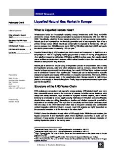
One question is who has power another is how to model market power. Consider the stylized structure in Figure 1, where one or more gas producers sell to a transmission or a distribution company, who resells to the final consumers. The numbered arrows represent exertion of market power. 1, for example, means that producers exploit market power versus a price-taking transmitter, while 2 represents the opposite when a transmission company exploits its power versus a price-taking producer. While one may observe that several or even all these relationships co-exist in a particular industry, economic theory makes the modeling of some combinations difficult. The problem is whether the theory provides a (locally) unique solution or not.

Figure 1. Illustration of combinations of market power. Gas producers

1

2

Transmission companies

Consumers 4

3

Within non-cooperative game theory, it is well known how to model 1 (only). This is an oligopoly of producers selling to price-taking transmitters, i.e., the Nash-Cournot model. 3 is the previous model turned upside down, i.e., an oligopoly of transmission companies, and although one does not see many applications, it is conceptually sound. Combination 1&2 describes a situation of successive market power, where producers sell to price-taking transmitters, who in turn exploit their power over price-taking customers. Combination 2

2&3 is about a company that has market power in both factor and product markets. It can be generalized to an oligopolistic setting.

Combination 1&3 signals a situation where both sides of a market have power versus the other. This is referred to as a bilateral monopoly. Rather than a unique solution, it involves a continuum of solutions. The impasse may be resolved by using the Nash bargaining solution concept of cooperative game theory. This theory, however, is not as easily available as the non-cooperative theory for large, detailed, numerical models. Thus, one has to decide which features are essential to model, and which are not. Our model employs non-cooperative game theory, whereby we cannot model the explicit exertion of market power of two opposing agents in a market. There are indirect ways to analyze the realities of 1&3, though, and we return to such analysis below.

The features mentioned above, in addition to the number of details in each dimension, are relevant for some analyses. Even though present day PCs have an enormous computing capacity, one has in practice, however, to abstain from bringing in every dimension in gory detail. If not for other reasons, one should acknowledge that such a model is meant to support decisions and thus has to be transparent enough for the user to understand what is going on inside the model.

Except for splitting the year into two sub-periods, we have dropped the intertemporal aspect. Recognition of T periods would make a model on the order of T times larger in terms of variables etc. Thus the time dimension is a very costly one to include in combination with other details.2 Our model describes activities over two seasons of a future year. It observes 8 agents producing from a total of 22 different fields, selling through transmission companies to 18 regions with 3 consumer groups each. In addition, there are storage capabilities between seasons. We do not model any explicit network. This model has a total of 3800 variables. (See Eldegard et.al. 2001.)

The remainder of the paper is structured as follows. Chapter 2 discusses modeling of behavior, which is embedded in a spatial model in chapter 3. In chapter 4 two types of transportation models are distinguished. Chapter 5 reviews some previous attempts at modeling natural gas markets. 2

Chapter 5 reviews previous attempts at modeling the gas market, and it the pattern is clear. When the analyst includes time in his model, other details are kept at a minimum.

3

2. Behavior In many markets suppliers have the ability to influence price, and their exertion of such power is an essential feature of the market. Adopting an assumption of price-taking behavior may seriously distort model solutions. Of course, whether a particular market, like the European natural gas market, is best modeled as non-competitive rather than a competitive one, is an empirical question. Rather than delve on this question, we will illustrate some major differences in the solutions for these alternative model assumptions.

We consider the market for a homogeneous product and assume that producers make quantity decisions3. For ease of exposition, let us first assume there is one non-segmented market. Let i denote producer, i=1,...,n, and further let

xi and Ci(xi) denote his quantity and total cost of producing it, let p(X)

denote the market price as a function of total supply, i.e., X = Σi xi, and let

πi(x) = p(X)xi - Ci(xi) denote his profits, where x = (x1,…,xn) is a vector of decision variables for all n producers

The profit maximization problem of producer i, is then

(1)

maximize πi(x) = p(X)xi - Ci(xi),

i=1,…,n.

We observe that through the vector x, his maximization problem is a function of all rivals’ decision variables as well. Provided xi > 0, his first order (necessary) condition for a profit maximum is ∂πi/∂xi = p + [(∂p/∂x1)(∂x1/∂xi) + (∂p/∂x2)(∂x2/∂xi) + ... + (∂p/∂xn)(∂xn/∂xi)]xi - ∂Ci/∂xi =4 p + p’[ 1 + Σk≠i (∂xk/∂xi)] xi – ci’ (2)

= {p + p’[1 + θ] xi} - ci’ = 0.

3

In a homogeneous good model, the assumption of price setting is unattractive. It could imply a solution where price equaled marginal cost, which does not seem to match realities, or it might even cause nonexistence of solutions. Quantity setting seems to match realities of contracts better, and we follow most analysts assuming quantity setting and Cournot behavior. 4 Homogeneity of product implies ∂p/∂x1= ∂p/∂x2 = ... = ∂p/∂xn = p’, i.e., a change in any supplier’s volume, affects price equally.

4

The term θ ≡ Σk≠i (∂xk/∂xi) represents the sum of rival’s responses to the marginal quantity of producer i. It is called conjectural variations signaling that producer i holds conjectures about his rival’s responses. The entire bracketed term is marginal revenue. The condition is for optimal production to be at a level where marginal revenue equals marginal cost.

From (2) we may extract several behavioral types. The Nash Cournot hypothesis is that producer i conjectures (∂xk/∂xi) = 0, k≠i. Thus (2.1)

∂πi/∂xi = {p + p’xi} - ci’ = 0.

The price taker ignores his influence on price, i.e., regards p’ = 0, in which case we are left with the condition that price equals marginal cost, (2.2)

∂πi/∂xi = p - ci’ = 0.

The most general behavior is the ‘conjectural variation’-case where (∂xk/∂xi) can be anything, whereby θ ≠ 0 in (2). Our final example is a cartel of producers, i ∈ Λ ⊆ N = {1, 2,…, n}, i.e., a subset of the n producers5. Each member i of the cartel consider the aggregate production of the cartel when he adjusts his own production (2.3)

∂πi/∂xi = {p + p’(Σk∈Λ xk)} – ck’ = 0.

Non-negative sales In applications we have to allow for the possibility that a producer does not find it profitable to operate in the market. That is, the maximization problem of producer i is maximize

πi = {p(X)xi – Ci(xi)}

subject to

xi > 0,

i = 1,…,n.

The corresponding first order (Kuhn-Tucker) conditions of a Cournot player are: ∂πi/∂xi = {p + p’xi} - ci’ < 0, (3)

xi > 0,

and

xi [{p + p’xi} - ci’] = 0, 5

i =1,...,n.

We assume that this aggregate player behaves as a Nash Cournot player against non-members.

5

The first part of (3) says that marginal profit has to be non-positive! Assume the opposite, namely that {∂πi/∂xi} was positive in equilibrium. Then, profits could be increased by expanding sales, indicating that the initial position was no equilibrium. Hence in equilibrium, where by definition all profit opportunities are exploited, marginal profit has to be non-positive. The second condition is that the flow has to be non-negative. Thirdly, if a flow is positive, the marginal profit is zero, while on the other hand, if marginal profit is negative, the flow is zero. It simply is not profitable to sell even the first unit.

The first order conditions (3) stem from n different optimization problems that are interrelated. Mathiesen (1985) suggested that this problem could be solved by the SLCPalgorithm6, which today is available as the MCP-solver in GAMS.7

Optimization approach Another and much more popular approach is to try convert equilibrium conditions like (3) into a single optimization problem.8 The question is, under what conditions does there exist a (fictitious) function Π(x) with the property that:

(4)

∂Π/∂xi = ∂πi/∂xi, i=1,...,n ?

If such a function Π(x) exists, the game of n agents maximizing individual profit functions would be equivalent to a problem where one single agent maximizes this fictitious objective. In general, the function Π(x) exists if and only if the n first-order conditions, like (3), are integrable.9

Proposition. (Slade, 1988). In a game with payoff functions that possess first and secondorder derivatives, the fictitious objective function Π(x) exists if and only if the individual profit functions πi(x) can be written: (SL)

πi(x) = π(x) + Ωi(xi) + Θi(x-i).

x-i denotes all variables except xi. When (SL) is satisfied, Π(x) = π(x) + Σi Ωi(xi).

6

The acronym stands for A Sequence of Linear Complementarity Problems, describing a Newton-like iterative process where the linear conditions in each step are solved by Lemke’s method. 7 GAMS is a software package for a variety of optimization problems. It has become an industrial standard. See www.gams.com for details on content and how to obtain this package. 8 Samuelson (1952) originated this approach, demonstrating that in order to compute the competitive equilibrium one could maximize the sum of consumers’ and producers’ surpluses. (See below.) 9 Refer to the integrability of demand in microeconomic theory. See e.g. Varian (1992).

6

For the homogeneous product Cournot model (as (3)), the SL-condition requires that inverse demand be linear, i.e., p = a – bX. The optimization approach is therefore available for the Cournot-model, provided one applies linear demand functions.

The optimization approach has been widely adopted and is by far the most popular formulation of a partial equilibrium model.10 We observe, however, that it may not be easily employed in a non-competitive regime.

10

There is a large literature on spatial and temporal equilibrium models. See e.g. Takayama and Judge.

7

3. The generalized transportation model Consider a market for a homogeneous commodity, e.g. oil, natural gas, coal, grain, paper, a metal like aluminum, etc. As a starter, assume there are many producers and consumers in this market such that one may reasonably apply price-taking behavior. Producers may be aggregated into supply-curves (industry cost curves) per region, and likewise, consumers may be aggregated into demand functions per region or segment. Let there be n producing and m consuming regions, and let i and j denote producing respectively consuming region. Further let

ci

denote the marginal cost of production in region i,

si(ci)

denote supply from producing region i,

xij

denote sales from producing region i to consuming region j,

tij

denote the unit transportation cost from i to j,

pj

denote consumer price in consuming region j, and

dj(pj) denote demand in consuming region j. A competitive equilibrium in this market is characterized by three sets of conditions.

Supply balance: (5.1)

si(ci) - Σj xij > 0,

ci > 0,

ci[si(ci) - Σj xij] = 0, i=1,…,n.

pj > 0,

pj[Σi xij - dj(pj)] = 0, j=1,…,m.

xij > 0,

xij[ci + tij – pj] = 0, i=1,…,n, j=1,…,m.

Demand balance: (5.2)

Σi xij - dj(pj) > 0,

Price formation: (5.3)

ci + tij – pj > 0,

The interpretation of (5) is as follows: (5.1) and (5.2) are conditions on regional balances of supply and demand and the corresponding prices, while (5.3) relates to the profitability of trade flows between regions.

8

In (5.1), the production of region i has to be at least as large as its total sales; marginal cost – interpreted as the supply-price – has to be non-negative, and finally, if the supply price is positive, production equals sales.

(5.2) says that consumption in region j cannot be larger than incoming flows from supplying regions; the price has to be non-negative, and finally, if the price is positive, consumption equals total inflow.

(5.3) parallels condition (3). In order to obtain symmetry in (5), the first inequality is multiplied by –1. The negative of marginal profit on sales from supply-region i to consuming region j has to be non-negative. Next, the flow has to be non-negative; and finally, if a flow is positive, its marginal profit is zero, while on the other hand, if marginal profit is negative, the flow is zero. As we shall see below, zero will be a typical outcome for a large number of flows in a competitive equilibrium.

Consider now maximizing the sum of consumers’ and producers’ surpluses. Let ci(Qi) denote the marginal cost of producing Qi in region i, and bj(Zj) denote the marginal willingness to pay for consumption Zj of region j. The optimization approach to solving (5) can then be stated as z

Q

(6.1)

Maximize {Σj ∫ j bj(uj)duj - (Σi ∫ i ci(vi)dvi + Σi Σj tij xij)}

(6.2)

subject to

Σi xij > Zj,

Σj xij < Qi,

xij > 0.

The objective (6.1) represents consumers’ and producers’ surpluses as the difference between consumer evaluation of consumed volumes (Zj) and costs of production and transportation. Samuelson (1952) demonstrated that the first order conditions of (6) implied the solution to (5). Observe that if Qi and Zj are constants, i.e., exogeneously stipulated production and consumption quantities, Q’i and Z’j, the two integrals in (6.1) are not well defined – as demand and supply-curves are vertical. (6) then reduces to minimizing transportation costs subject to constraints. This is the well-known transportation model of linear programming Maximize - Σi Σj tij xij

subject to Σi xij > Z’j, Σj xij < Q’i, and xij > 0.

9

Non-competitive behavior Assume now that producer i is a single decision unit and not an aggregate of several individual producers. Assume further that this agent behaves according to the Nash hypothesis when selling in region j, i.e., he observes his influence on price (pj) and conjectures that other producers regard his quantity (xij) as given. The first order conditions for his profitable sale to region j are then

(5.3’) (ci + tij) – (pj + pj’xij) > 0,

xij > 0,

and

xij[(ci + tij) – (pj + pj’xij)] = 0, i=1,…,n, j=1,…,m. His marginal profit is now the difference between the marginal cost of production plus transportation and the marginal revenue. This has to be non-positive.

Let us compare implications of different behaviors. The price-taker sells to markets where his net-back price [pj - tij] is maximized, i.e., his decision rule is

(7.1)

sell to region j when pj - tij > pk - tik for all k≠j. See (5.3).

Knowing that his supply affects the price, the Nash player considers the net-back of marginal revenue [(pj + pj’xij) - tij], i.e., his decision rule is

(7.2)

sell to region j when [(pj + pj’xij) - tij] > [(pk + pk’xik) - tik] for all k≠j.

This net-back is an explicit function of his volume, and he adjusts xij so that sale to market j may be profitable. Hence, for markets far away, where net-back price will be low, he will only sell a little. The following example will illustrate the implications for trade volumes of rules (7.1) vs (7.2).

10

A numerical example Consider a market consisting of 4 individual producers and 6 consuming regions. For the illustration of consequences of different behavioral assumptions we shall employ linear (inverse) demand and marginal cost functions

pj = Aj + Bj Zj,

j = 1,…,6, and

ci = ai + bi Qi,

i = N, D, R, A.

Let Aj = 20, Bj = -0.25, ai = 1, and bi = 0.1, i.e., we assume that demand and marginal cost are equal across regions. Unit transportation costs are shown in Table 1.

Table 1. Unit transportation cost N D R A

1 2 1 3 3.5

2 2.5 1 4 4

3 3 1.5 3 3

4 3 2 2 2.5

5 4 3 2.5 1.5

6 4 2.5 3.5 2

For this model we have computed the competitive and the Cournot equilibria. They differ in several respects. At the aggregate level, the competitive equilibrium has a larger quantity (257 vs 212) and a lower (average) price (9.3 vs 11.2). See Tables 2 and 3. These are well known facts. We observe that even though demand and marginal cost functions are the same, unequal transportation costs make regional consumption and individual production volumes differ. This is also fairly intuitive. Distance matters.

Observe that volumes and prices vary much more across regions in the competitive equilibrium than in the Cournot equilibrium. The largest volume and highest price are 11 respectively 13% above the smallest volume and lowest price in the competitive equilibrium. The corresponding numbers in the Cournot equilibrium are 6 and 5%. We know that price variation between regions in a competitive equilibrium is bounded by differences in transportation costs. It is interesting to observe that price differences in the Cournot equilibrium may be considerably smaller.11

11

Of course, in this numerical example with identical demand, price elasticities are equal between regions in benchmark, namely –1, and Cournot-players have no incentive to price discriminate. However, even when elasticities differ somewhat between regions and vary between -0.6 and -1.4 with an average of -1, price differences are smaller in the Cournot equilibrium. For larger differences in elasticities though, price variation becomes larger in the Cournot equilibrium.

11

Table 2. Volumes and prices of the competitive equilibrium From/ to 1

N D R A Sum Price

45.1

45.1 8.72

2 6.5 36.6

43.1 9.22

3 5.5 35.6

41.1 9.72

4

5

6

44.5

14.3 28.3 42.5 9.38

40.5 40.5 9.88

44.5 8.88

Sum 57.2 72.2 58.8 68.8 257 9.28

Table 3. Volumes and prices of the Nash-Cournot equilibrium From/ to 1

N D R A Sum Price

11.7 12.2 7.5 4.8 36.2 10.94

2 11.3 13.8 5.1 4.4 34.6 11.34

3 8.5 11.0 8.3 7.6 35.4 11.14

4 7.7 8.2 11.5 8.8 36.2 10.94

5 4.9 5.4 10.7 14.0 35.0 11.24

6 5.7 8.2 7.5 12.8 34.2 11.44

Sum 50.0 58.9 50.6 52.4 212 11.17

The more spectacular difference between these equilibria is the rather diverge trade patterns, with 9 positive flows in the competitive equilibrium and 24 in the Cournot equilibrium12. In general and unless unit transportation costs (tij) of producer i differ considerably between regions, a Cournot producer will supply all regions. The pricetaking producer, however, supplies only a few neighboring regions. The rationale of the competitive equilibrium is to provide commodities at the lowest cost. Thus, a competitive equilibrium in the European gas market for example, would never have Norway supplying Italy or Spain, and at the same time Algeria supplying Belgium or Germany. Such a solution would imply ‘cross-hauling’ and a waste of resources.13 It characterizes, however, the Cournot equilibrium, and to some extent the present gas market.14

Another immediate result of the competitive equilibrium is the price-pattern between regions. For an active supplier, the market price increases with distance and transportation cost to the market. The price covers his combined costs of production and transportation. Seen alternatively, his net-back prices are equal for the markets where he sells. Producer N, for example, has net-back prices 6.72, 6.72, 6.72, 5.88, 5.38 and 5.88 from markets 1 to

12

The Cournot equilibrium may have nm positive flows, while the competitive equilibrium has at most (n+m-1) positive flows. 13 Of course, even though contracts involve sales from North to the South and vice versa, transmission companies may avoid actual cross-hauling, so that flows do not follow contracts. Mathiesen (1987) included such an option in the Statoil model. 14 In the context of this model, the present European natural gas market has about 20 positive flows. Recent developments like Norway selling to Spain and Poland indicate that at present producers do not behave as price-takers. It seems that the Cournot model provides a better fit.

12

6, and he sells to markets 1, 2 and 3. See (7.1). Observe, however, that the sales pattern where both producer N and D sell to markets 2 and 3, signals there are multiple solutions. Alternative solutions are obtained by shifting Ns combined sales into either of these markets and shifting in opposite direction a similar volume for D. Table 4 displays these two alternatives for N and D and markets 2 and 3. Other flows of the competitive solution of Table 2 are unaffected.

Table 5. Alternative flow patterns of the competitive solution From/ to N D

2 12 31.1

3 0 41.1

2 0 43.1

3 12 29.1

Assume for example, that Ds transportation cost of supplying market 2 was 0.99 and not 1. Compared to the previous situation, D has a slight comparative advantage over N in serving market 2. Then, the alternative where N serves market 3 and not 2, would be the unique equilibrium. His net-back price from market 3 is still 6.72, while that from market 2 has dropped to 6.71, and he does not sell there.

The Cournot equilibrium equalizes net-back marginal revenues, while net-back prices may differ between the markets that a producers supplies. See (7.2). Producer N’s net-back prices from the six markets are 8.94, 8.84, 8.14, 7.94, 7.24 and 7.44, and he sells to all six markets. It is noteworthy that he sells to markets with a net-back price difference of 1.70, while the price-taker may not sell to markets where the difference is as low as 0.01.15

Based on the observation that price exceeds supply cost in the Cournot equilibrium, it has been suggested that by allowing mark-ups on cost, the competitive model can replicate the Cournot equilibrium. Inspection of condition (5.3) and (5.3’) reveals that a mark-up-factor (λij) in such case has to be λij = - (pj’xij)/(ci + tij),

i = 1,...,n, and j = 1,...,m.

There are two problems here. One is the information content, which is demanding as these mark-ups differ both by producer and market. In fact, the entire Cournot flow-matrix (xij)

15

Who sells where in the competitive equilibrium is very sensitive to relative transportation costs. Production and consumption volumes, however, change by less than 0.1%. The flows in the Cournot equilibrium are much more stable. The largest change in an individual flow is 0.5% in this example.

13

has to be known, and if mark-ups are not accurately known, there is no way a competitive model can replicate the Cournot equilibrium. The next problem is related to the model, its solver and the structure of the solution. Assume that the Cournot equilibrium is known and compute parameters λij, i.e., constants, as distinguished from functions of variables. Solve (6), modified by mark-ups (1+λij) on cost. This model has an infinity of solutions. One is the Cournot equilibrium. Another has the trade pattern of Table 2, only flows will be smaller. With multiple solutions, it is unclear which solution that will be reported by the solver. Of course, by computing the net-back prices, one may learn that a trade pattern like that of the Cournot solution may be optimal.

14

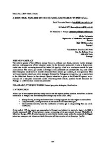
4. Network Transportation in the previous model can be pictured as in Figure 2a. Supplier i can sell in any market j, and there is no explicit mention of how transportation is done. Only unit transportation cost tij is represented. This cost is assumed to be the lowest cost of shipping a unit from i to j. This may be denoted a transportation type model.

Figure 2a. Transportation type model.

S upply regions N

Figure 2b. Network type model

Dem and regions 1

N

D

2

1

2 D

3

4

R

3 4

5

6

R 5

A A

6

Natural gas is a commodity where volumes have to follow a designated transportation system, a network of pipelines, although the gas may flow along any of a number of different routes.16 Figure 2b displays the same industry where producers labeled N, D, R and A, insert flows into the network and consuming regions labeled 1-6, extract gas. Gas from N to market 6, for example, may flow along one or more of several routes, e.g. N-2-3-6, N-1-3-6 or N-1-4-5-6. We call this a network type of model.

Also in network industries one may find the cheapest route of transportation between two regions, e.g. between N and 6, and use the corresponding unit cost in a transportation type model of the actual market. As will be seen below, most of the reviewed analyses employ this type of model. The critical issue is whether there are features of the network that are not represented by such unit costs.

Restricted capacities of individual pipelines are certainly not represented in the transportation model. Figure 3a illustrates the case of a pipeline with unit cost, or tariff, t 16

Along with pipelines we also include LNG-routes with harbors and associated liquefaction.

15

and a given maximal capacity K (in terms of m3 flow per time period). As long as the total flow on this pipeline is below K, e.g. demand for capacity is D1, there is no problem. Total shipments X are allowed at the unit cost t. If demand for capacity at tariff t exceeds K like in case D2, however, some shipments cannot be executed, and there has to be rationing. The simplest rationing, in terms of modeling, is to use the shadow price λ of the scarce capacity K. That is, the price per unit transported through the pipeline is increased to (t+λ), at which this market17 is cleared. Assume that the value of λ is known. Then tariff t could be replaced by (t+λ) and the capacity constraint disregarded. The aggregate flow in the optimal solution would now equal the capacity.

Figure 3a. Pipeline pricing

Figure 3b. Pipeline pricing

Price

Price

D2 D1

t3 t+

λ

t2

t

t1 X

K

Agg.flow

Agg.flow

The shadow price depends, however, on the optimal solution of the market model. Hence, the shadow price cannot be known in advance, although the value for a particular pipeline may turn out to be fairly stable between various scenarios.

The critical question is whether the time horizon of the analysis is sufficiently long, so that capacities can be increased in order to be non-binding. If so, one may assume that necessary investments will be made to accommodate planned flows, and one may employ a transportation type model. If, on the other hand some capacities will be constraining within the time horizon, there may be no escape, but model the actual network. Obviously, one will have to aggregate details also in this dimension of the market and represent only the major transmission lines.

There are two issues related to behavioral types when modeling a network and individual pipelines. One is about gas sellers the other is about pipeline owners. The first is about

17

We may consider the supply of and demand for capacity in a given pipeline as a market.

16

how the network and its flows are modeled. The traditional model balances aggregate flows into and out of a given node. E.g. the aggregate flow into node 4 (in Figure 2b) has to equal the aggregate flow out of this node. In the dual representation, the model sums the cost per unit gas injected into the network and unit cost of transportation18 along the various pipelines into a price of delivering gas at any node. And oppositely, it provides net-back prices to a supplier from any market.

In an application with several suppliers injecting their flows, possibly at different nodes, these flows mix and the model disregards who are the owners (sellers). This is of little importance if all sellers are price takers. (See (5.3).) Suppliers obtain the necessary information, namely the market prices, and they can compute their net-back prices of supplying the various markets and hence chose where to sell. (See (7.1).)

When supplier i is not a price taker, however, in particular if he is a Nash-Cournot player, we also need information on his supplies to market j (xij). (See (5.3’).) In order to provide this information, the model has to keep track of individual flows.19 Such a model easily becomes much larger than the traditional version. In the discussion related to Figure 3a, we stated that at a tariff (or price) (t+λ), the market involving supply of and demand for capacity of the pipeline was cleared. Implicitly, we then assumed that the owner of the pipeline stipulated his price t independent of actual demand or stipulated (t+λ) taking demand, or the marginal willingness to pay for this capacity, as given. The price-taking assumption may be dubious when for example a pipeline owner has market power and is in a position to set his price optimally. As mentioned in the introduction, however, non-cooperative theory does not provide a unique solution when both sides of a market enjoy market power. (Here a supplier of transmission capacity and a gas producer demanding such capacity.) By computing the equilibrium for different tariffs (t1, t2, t3,..), however, one may analyze a pipeline owner’s pricing and the consequences for aggregate transportation, consumption, his profits, etc. See Figure 3b. By such trial and error, we can search for his optimal tariff.

18 19

Observe that this unit cost may include the shadow price when a capacity is binding. Mathiesen (1987) constructed such a model for the European natural gas market.

17

5. Previous modeling efforts of gas markets An early effort is the Gas Trade Model developed in the Systems Optimization Laboratory at Stanford around 1980 (Beltramo et.al. (1986)).20 This is a multi-regional transportation type model of the North American market. It assumes price-taking behavior in supply and demand. Berg (1990) employed a version of the model for an analysis of increased Canadian supply to the US market. Boucher and Smeers (1984) applied this structure for an analysis of the European market.

Mathiesen et.al. (1987), focusing on the exertion of market power on the selling side, extended this model structure by allowing various kinds of seller behavior, viz. (2.1), (2.2), and (2.3). Brekke et.al. (1987) suggested that applying such a static (or one-period) model to analyze some 10-15 years into the future, seriously misrepresented the investment process over this time span. They built an intertemporal model where suppliers engaged in a dynamic game observing previous actions and reacting to them. Because of the time-dimension and added complexity in the strategy-space, they condensed other aspects. For example, they considered only one aggregate European excess demand - net of indigenous production. They disregarded the UK market and subsumed Dutch production in indigenous production, thus considering a game between the three players: Norway, Algeria and the Soviet Union.

Bjerkholt et.al. (1989) studied market power exerted by the transmission companies and possible effects of a deregulation in terms of third party access to pipelines of the European gas market by 1992. They did not formulate a model for optimal tariffs. Cf. our discussion related to combination 1&3 in Figure 1. Hoel et.al. (1987), however, modeled a cooperative game between sellers and buyers, represented by transmission companies, in the gas market. Golombek et.al. (1995, 1998) consider aspects of the deregulation process of European energy market. (See Smeers (1997).) The models are of a transportation type and consider production and consumption in various regions. Golombek et.al. (2000) include the electricity market as well.

20

A similar type of model was developed at the Energy Laboratory at MIT and applied in three separate analyses of North America, Europe and far East Asia.

18

Mathiesen (1987) extended the Mathiesen et.al. (1987) model to allow for a network of transmission lines. The model was constructed for Statoil to simulate various scenarios in the European gas market. To facilitate such analyses, the model was embedded in an interactive program and presented as a decision support system.21

Using the network model, Mathiesen (1988a) demonstrated the importance of the spatial dimension in combination with strategic behavior. Particularities of the geography are lost when assuming sale at a central destination in Europe. Selling strategies for individual producers may look very different in a spatial and a non-spatial model, and the sales pattern of the competitive and the non-competitive equilibria also differ tremendously, as illustrated above. The spatial aspect was important also in the analysis of Norwegian sales to UK (Mathiesen, 1988b).

Tandberg analyzed the potential for gas in Scandinavia (Tandberg, 1990, 1992), where he studied investments in a pipeline system to supply Sweden. His analysis employed a model that considered three forms of energy. Natural gas and electricity were modeled to flow from gas fields or power plants to consumers through separate networks, while fuel oil was supplied at a unit cost. Energy demand originated in six consumer groups in twelve regions, and the individual supplier of natural gas and electricity might be a pricetaker or a Nash oligopolist. (Mathiesen, 1990).

Øygard and Tryggestad (2001) consider the deregulation of the European gas market using the McKinsey model. Judging from their non-technical description and a presentation by Keller (2001), presumably of the same model, it seems to be a fairly detailed network-type model with large numbers of production fields, pipelines, consuming regions and consumer types, but where suppliers and other agents are price takers. It may seem that the behavioral dimension is sacrificed for details. Most likely this is an LP-model with staircase graphs representing supply and demand. This may be good strategy for some kind of analyses. As seen in the numerical illustration, however, the trade pattern of such a model, or changes in trade pattern, may be next to non-informative. One should appreciate the insights gained from a combination of behavior and geography (Mathiesen, 1988a), or behavior and time (Brekke et. al. 1987), both of which combinations are not available in the McKinsey model. 21

A similar package is developed for Oljedirektoratet. (Helming and Mathiesen, 1993). The Statoil model is extended, its database is updated and the interactive program improved. (Fuglseth and Grønhaug, 2001).

19

Referanser. Beltramo, M.A., et.al., A North American Gas Trade Model (GTM), The Energy Journal, vol 7, 1986. Berg, M., Økt tilbud av naturgass fra Canada til USA: En markedsstrategisk analyse, Working paper 16/90, Senter for Anvendt Forskning, Bergen, 1990. Bjerkholt, O. et.al., Gas Trade and Bargaining in Northwest Europe: Regulation, Bargaining and Competition, Disc. paper 45/89, Central Bureau of Statistics, Norway, 1989. Boucher, J. and Y. Smeers, Simulation of the European Gas Market up to the Year 2000, Discussion paper 8448, CORE, Louvain-la-Neuve, 1984. Brekke, K.A. et.al., A Dynamic Supply Side Game Applied to the European Gas Market, Discussion paper 22/87, Central Bureau of Statistics, Norway, 1987. Eldegard, T., O. Godal and J. Skaar, A Partial Equilibrium Model of the European Natural Gas Market, SNF Report 52/2001, Stiftelsen for samfunns- og næringslivsforskning, Bergen, 2001. Fuglseth, A. M. and K. Grønhaug, Can computerised market models improve strategic decision-making?, Norges Handelshøyskole, 2001. Golombek, R. and S. Kverndokk, Modeller for elektrisitets- og gasmarkedene i Norge, Norden og Europa, Notater 96/45, Statistics Norway, 1996. Golombek, R., et.al, Effects of Liberalizing the Natural Gas Markets in Western Europe, The Energy Journal, Vol 16, No. 1, 1995. Golombek, R., et.al, Increased Competition on the Supply Side of the Western European Natural Gas Market, The Energy Journal, Vol 19, No. 3, 1998. Golombek, R., et.al, Deregulering av det vest-europeiske gassmarkedet - korttidseffekter, Rapport 5/2000, Ragnar Frisch Centre for Economic Research, Oslo. Helming, R. and L. Mathiesen, OLGA: En modell og et interaktivt system for analyser av det europeiske marked for naturgass, SNF Rapport 82/93, Stiftelsen for samfunns- og næringslivsforskning, Bergen, 1993. Hoel, M. et.al., The market for natural gas in Europe: The core of a game, Memo 13, Department of Economics, University of Oslo, 1987. Keller, L., BP. A presentation at NPF, Trondheim, May 28, 2001. Mathiesen, L., Computational experience in solving equlibrium models by a sequence of linear complementarity problems, Operations Research, Vol 33, 1985. Mathiesen, L., GAS: En modell og et interaktivt system for analyser av det vest-europeiske marked for naturgass, Report nr. 3, Senter for Anvendt Forskning, Bergen, 1987. Mathiesen, L., En modellramme for analyser av regionale markeder for gass og elektrisitet, Working paper 38/90, Senter for Anvendt Forskning, Bergen, 1990. Mathiesen, L., Analyzing the European Market for Natural Gas, Working paper 37/88, Senter for Anvendt Forskning, Bergen, 1988a.

20

Mathiesen, L., Om strategisk tilpasning for Norge i det britiske marked, Working paper 40/88, Senter for Anvendt Forskning, Bergen, 1988b. Mathiesen, L. et.al., The European Natural Gas Market: Degrees of Market Power on the Selling Side, in Natural Gas Markets and Contracts, R.Golombek et.al. (eds), Amsterdam: North Holland Publishing Company, 1987. Samuelson, P., Spatial Price Equilibrium and Linear Programming. American Economic Review, 42, 1952. Slade, M., What does an oligopoly maximize, Discussion paper 88-35, Department of Economics, University of British Columbia, 1988. Smeers, Y., Computable Equilibrium Models and the Restructuring of the European Electricity and Gas Markets, The Energy Journal, Vol 18, No 4, 1997. Takayama, T. and G.G. Judge, Spatial and Temporal Price Allocation Models, Amsterdam: North Holland Publishing Company, 1971. Tandberg, E., Naturgass i det nordiske energimarkedet, Report 4/90, Senter for Anvendt Forskning, Bergen, 1990. Tandberg, E., Introduction of natural Gas in the Scandinavian Energy Market, HAS-oppgave (Master Thesis), Norges Handelshøyskole, 1991, and working paper 53/92, Stiftelsen for samfunns- og næringslivsforskning, Bergen, 1992. Varian, H., Microeconomic Analysis, Norton, 1992. Øygard, S.H. and J.C. Tryggestad, Volatile gas, McKinsey Quarterly, No. 3, 2001.

21