The Allocative Cost of Price Ceilings in the U.S. Residential Market for Natural Gas Lucas W. Davis

Lutz Kilian∗

November 2009

Abstract A direct consequence of imposing a ceiling on the price of a good for which secondary markets do not exist, is that, when there is excess demand, the good will not be allocated to the buyers who value it the most. The resulting allocative cost has been discussed in the literature as a potentially important component of the total welfare loss from price ceilings, but its practical importance has yet to be established empirically. In this paper, we address this question using data for the U.S. residential market for natural gas which was subject to price ceilings during 1954-1989 and is well suited for such an empirical analysis. Using a householdlevel, discrete-continuous model of natural gas demand, we estimate that the allocative cost in the U.S. residential market for natural gas averaged $4.1 billion annually, nearly tripling previous estimates of the net welfare loss to U.S. consumers. We quantify the evolution of this allocative cost and its geographical distribution during the post-war period, and we highlight implications of our analysis for the regulation of other markets.

Key Words: Price Ceilings, Allocative Cost; Natural Gas Regulation; JEL: D45, L51, L71, Q41, Q48 ∗ (Davis) Haas School of Business, University of California, Berkeley and National Bureau of Economic Research (Kilian) Department of Economics, University of Michigan and Centre for Economic Policy Research. Comments from Jim Adams, Jim Hines, Kai-Uwe K¨ uhn, Peter Reiss, Dan Silverman, Gary Solon, the editor, two anonymous referees and numerous seminar participants substantially improved the paper.

1

Introduction A large literature in economics has examined the welfare costs of price ceilings. Among the

markets that have received the most attention are rental housing, telecommunications, insurance, energy, and health care.1 In traditional welfare analysis, price ceilings reduce the quantity transacted below the competitive level, imposing deadweight losses on both buyers and sellers. In this paper we concentrate on an additional component of welfare loss that is often ignored. Notably, when there is excess demand for a good for which secondary markets do not exist, a welfare loss occurs when the good is not allocated to the buyers who value it the most. This allocative cost has been studied, for example, by Glaeser and Luttmer (2003), but its practical importance has yet to be established empirically.2 Our analysis focuses on the U.S. residential market for natural gas. Anecdotal evidence suggests that price ceilings imposed in this market during the post-war period led to severe misallocation of natural gas across households. While some households were enjoying access to cheap pricecontrolled natural gas, other households were locked out of the market altogether as new residential connections were unavailable in many parts of the country.3 Many of these households without access to natural gas may well have been willing-to-pay more than households with access, but there was no mechanism that allowed such welfare-improving reallocations to occur. The allocative cost of these price ceilings refers to the total increase in welfare that could have been obtained by reallocating natural gas to the households with the highest willingness-to-pay. The natural gas market is a good candidate for an empirical study of allocative costs for several reasons. First, natural gas is a homogeneous good, eliminating the concerns about differences in quality that complicate the estimation of allocative costs in other markets. Second, whereas secondary markets may act to mitigate the costs of misallocation in some markets such as rental housing, there are no resale markets for natural gas. Third, the residential market for natural gas 1

See, for example, Hayek (1931), Olsen (1972), Smith and Phelps (1978), Raymon (1983), Frech and Lee (1987), Suen (1989), Deacon and Sonstelie (1989, 1991) and Frech (2000). A closely related literature studies the welfare costs of minimum wage legislation in labor markets. See, e.g., Holzer, Katz and Krueger (1991) and Card and Krueger (1994). 2 The problem of allocative costs is aptly described in Friedman and Stigler (1946). An early theoretical treatment can be found in Weitzman (1977). The analogous problem of misallocation due to minimum wages has been discussed as early as Welch (1974) and has been studied in Luttmer (2007). 3 As described in American Gas Association (1975, p. 67) the gas shortage caused widespread restrictions on new residential customers and severely limited expansion into new residential customer markets by many utilities. See also MacAvoy and Pindyck (1975, p. 2), Herbert (1992, p. 127) and American Gas Association (1976, p. 125). Related discussion can be found in MacAvoy (1971), Breyer and MacAvoy (1973), MacAvoy and Pindyck (1973), and MacAvoy (1983).

1

affects millions of consumers, suggesting that allocative costs could be very large. Fourth, this market was continuously regulated between 1954 and 1989 before experiencing complete deregulation.4 This allows us to observe market behavior both under regulation and in the absence of regulation. Fifth, the fact that some states remained unregulated throughout this period allows us to evaluate the out-of-sample fit of our model in settings where markets operate freely. Sixth, this market lends itself to empirical analysis, given the availability of unusually comprehensive household-level data by state and year as well as the corresponding state-level price data. We construct estimates of the allocative costs associated with the regulation of natural gas prices by exploiting the fact that by the 1990s, the natural gas market had been completely deregulated and, unlike during the period of regulation, all households wanting to adopt natural gas heating systems were able to make that choice. Our empirical strategy is to ask how much natural gas would have been consumed in 1950-2000 based on the household preferences revealed in the 1990s data, controlling for household demographics and housing characteristics that affect heating demand. Comparing households’ actual choices with what they would have liked to choose in an unconstrained world, as implied by an economic model of consumer choice, allows us to calculate physical shortages of natural gas and to measure the allocative cost of price ceilings. Our paper provides for the first time a detailed picture of the evolution of physical shortages in the U.S. natural gas market during the post-war period. Whereas previous studies have traditionally measured the degree of disequilibrium in the natural gas market using shortfalls in contractuallyobligated deliveries to pipelines, our measure of the physical shortage correctly incorporates not only demand from existing delivery contracts, but the unrealized demand from prospective new customers as well.5 This distinction is particularly important in the residential market because shortages were accommodated by restricting access to potential new customers rather than by rationing existing users. We find that during the period 1950-2000 demand for natural gas exceeded sales of natural gas by an average of 19.3%, with the largest shortages during the 1970s and 1980s. Compared to previous studies, we find that the shortages began earlier, lasted longer, and were 4

Sanders (1981), MacAvoy (1983), Vietor (1984), Braeutigam and Hubbard (1986), Kalt (1987), Bradley (1996) and MacAvoy (2000) describe the regulatory policies in the natural gas market since the 1950s. In Phillips Petroleum vs. Wisconsin the Supreme Court ruled that rising natural gas prices were against the interests of consumers in Wisconsin and charged the Federal Power Commission with establishing price ceilings. By the 1970s shortages were widely apparent, leading to the 1978 Natural Gas Policy Act which initiated a slow process of deregulation culminating in the complete elimination of price ceilings in 1989. 5 For example, Vietor (1984) reports that shortfalls in contractually-obligated deliveries to pipelines increased steadily beginning in 1970, reaching approximately 3 trillion cubic feet in 1976. This is a significant amount considering that total natural gas consumption in the U.S. in that year was 20 trillion. As large as these curtailments were, results from our model show that they understate the true level of disequilibrium in the market because they fail to account for demand from prospective new customers.

2

larger in magnitude. Physical shortages are important in describing the effect of price ceilings, but do not provide a measure of their economic costs. Using a household-level, discrete-continuous model of natural gas demand following Dubin and McFadden (1984) we estimate that the allocative cost from price ceilings averaged $4.1 billion annually in the U.S. residential market during 1950-2000.6 Because this allocative cost arises in addition to the conventional deadweight loss, our estimates imply that total welfare losses from natural gas regulation were considerably larger than previously believed. Moreover, our household-level approach provides insights into the distributional effects of regulation that could not have been obtained using a model based on national or even regional data. In particular, we are able to identify which states were the biggest losers from regulation. We show that the allocative cost of regulation was borne disproportionately by households in the Northeast and Midwest.7 Our analysis has several policy implications. First, regulators need to be aware that price ceilings only benefit consumers that have access to regulated markets. When there is a shortage of a good, not all consumers will have access to the market, and those who have access will not necessarily be the consumers who value the good the most. Second, the adverse effects of price ceilings can last much longer than the regulatory policies themselves. With natural gas, since households change heating systems infrequently, households who are barred from adopting natural gas heating systems because of a price ceiling will continue to use inferior technologies for years to come. This lock-in effect helps explain the persistence and the magnitude of the allocative costs that we find, and highlights the difficulty of predicting the duration of the effects of price regulation. Third, our analysis underscores the difficulty of determining in advance how the allocative cost of price regulation will be distributed geographically. The format of the paper is as follows. Section 2 demonstrates the existence of an allocative cost from price ceilings in addition to the conventional deadweight welfare loss for goods for which there is no secondary market. Sections 3 and 4 introduce our household-level model of demand for natural gas and discuss its empirical implementation. In section 5, we discuss the estimates of physical shortages as well as allocative cost and the out-of-sample fit of the model. Section 6 6

All dollar amounts are expressed in year 2000 dollars. Our analysis is germane to a substantial literature that examines regulation in the U.S. natural gas industry. Early studies such as MacAvoy (1971), MacAvoy and Pindyck (1973), Breyer and MacAvoy (1973) and MacAvoy and Pindyck (1975) document gas shortages in the early 1970s and use structural dynamic simultaneous equation models to simulate hypothetical paths for prices, production and reserves under alternative regulatory regimes. Several of these studies present estimates of the deadweight loss from natural gas price ceilings, but only Braeutigam and Hubbard (1986) and Viscusi, Harrington and Vernon (2005) discuss the issue of allocative cost. 7

3

contains concluding remarks.

2

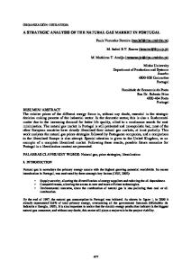
Price Ceilings and Allocative Cost Figure 1 describes the standard problem of imposing a price ceiling. At the competitive equi-

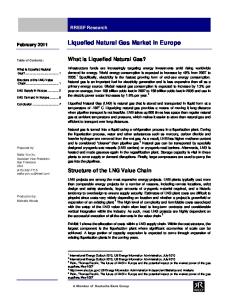
librium, the market clears with price P ∗ and quantity Q∗ . Now consider the effect of a price ceiling P ∗∗ imposed below P ∗ . The price ceiling reduces output to Q∗∗ . At this level of output demand D(P ∗∗ ) exceeds supply S(P ∗∗ ). Compared to the competitive equilibrium, households gain P ∗ deP ∗∗ from paying P ∗ − P ∗∗ less per unit but lose triangle bcd because of the decrease in quantity. Firms are unambiguously worse off, losing P ∗ deP ∗∗ because of the decrease in price and dce because of the decrease in quantity. Total deadweight loss is bce. The welfare cost of price ceilings, however, is not necessarily limited to this triangle. Upon further inspection it becomes clear that welfare losses will be limited to the deadweight loss triangle bce if and only if the good is allocated to the buyers who value it the most. Under efficient rationing, buyers represented on the demand curve between a and b receive the good, while those represented by the demand curve between b and f do not. In some markets it may be reasonable to assume that a good is allocated efficiently. For example, when there is a secondary market where goods can be resold, this secondary market ensures that buyers with the highest willingness to pay receive the good. However, in many markets such as the market for natural gas there is no mechanism that ensures that customers with the highest reservation price will receive the good. In these markets the welfare costs of price regulation also depend on how the good is allocated. Inefficient rationing imposes additional welfare costs. A commonly used benchmark in illustrating these additional welfare costs is the case in which goods are allocated randomly to buyers (see figure 2).8 The random allocation is inefficient because it does not allocate goods to buyers with the highest willingness-to-pay. At the price ceiling P ∗∗ , demand for the good is D(P ∗∗ ), but supply is only Q∗∗ . If supply is allocated randomly then only a fraction

Q∗∗ D(P ∗∗ )

of buyers with a reservation price above P ∗∗ will be able to buy the good. This

random allocation is depicted by the curve

Q∗∗ D(P ∗∗ ) D(P ).

Now, in addition to the deadweight loss,

bce, there is an additional welfare loss, abe, that is the result of the loss of efficiency from not allocating the good to the consumers with the highest reservation price. This additional welfare loss represents the “allocative cost” of regulation in this example. 8

This analysis follows closely Braeutigam and Hubbard (1986), Glaeser and Luttmer (2003) and Viscusi, Harrington and Vernon (2005).

4

In practice, the level of the allocative cost will depend not only on how the good is rationed, but also on the distribution of reservation prices across households. In the market for natural gas heterogeneity in reservation prices arises mainly for two reasons. First, there are differences across households in preferences for different types of heating systems. For example, households differ in how much they value the cleanliness and convenience of natural gas. Second, households differ in how much they value different heating systems because of technological considerations. Compared to electric heating systems, natural gas and oil heating systems are expensive to purchase but inexpensive to operate. As a result, households with high levels of demand for home heating tend to prefer natural gas and heating oil. The conventional deadweight loss depends on the location and shape of the demand curve as well as the location and shape of the supply curve. In contrast, the allocative cost only depends on the location and shape of the demand curve and the equilibrium level of price and quantities, but not on the shape of the supply curve. Accordingly, our analysis abstracts from the supply side of the natural gas market. A limitation of our approach is that we cannot calculate a conventional measure of deadweight loss. For estimates of the deadweight loss see MacAvoy and Pindyck (1975) and MacAvoy (2000). With our model we are able to simulate demand for natural gas at the prices actually observed in the market during this period and to calculate shortages, but we are not able to say what equilibrium price levels would have prevailed without price ceilings or under alternative forms of regulation. The latter question indeed is of no relevance for the measurement of the allocative cost.

3

Demand Model Residential demand for heating equipment and for heating fuels (natural gas, electricity, and

heating oil) is modeled as the solution to a household production problem. Households make two choices. First, households decide which heating system to purchase. Second, conditional on the choice of the heating system, households decide how much heating fuel to use. Joint discretecontinuous models of the form described in this section have been the standard for modeling energy demand at the household-level since Hausman (1979), Dubin and McFadden (1984) and Dubin (1985). Their approach of using a discrete choice model to model explicitly durable goods purchase decisions has been widely adopted by more recent studies of energy demand including Bernard, Bolduc and Belanger (1996), Goldberg (1998), West (2004), Feng, Fullerton, and Gan (2005),

5

Mansur, Mendelsohn and Morrison (2008), and Bento, Goulder, Jacobsen, and von Haefen (2009). Households choose which heating system to purchase by evaluating an indirect utility function of the form: uij = α0j + α1j pij + α2j wi + ij .

(1)

The utility for household i of heating system j is a function of pij , the price per unit of heat for heating system j, and wi , a vector of household and housing characteristics including heating degree days, household size, household income, number of rooms, and the number of units in the building. The error term, ij , captures unobserved differences across households’ preferences for particular heating systems. The parameter α0j incorporates heating-system specific factors such as purchase and installation costs as well as preferences for particular heating systems that are common across households. The parameter α1j reflects households’ willingness to trade off the price per unit of heat against other heating system characteristics, and the parameter vector α2j describes interactions between household characteristics and heating system alternatives. The specification allows households living in cold climates to prefer natural gas heating systems, for example. The probability that household i selects alternative k is the probability of drawing {i1 , i2 , ..., iJ } such that uik ≥ uij

∀j 6= k. We assume that ij has an extreme value distribution and is i.i.d.

across households and heating systems. Under this assumption, the choice probabilities take the well-known conditional logit form and the heating-system choice model can be estimated using maximum likelihood.9 Conditional on choosing a natural gas heating system, the demand function for natural gas is assumed to take the form: xi = β0 + β1 pig + β2 wi + ηi ,

(2)

where xi denotes annual consumption of natural gas measured in British Thermal Units (BTUs). Demand for natural gas depends on pig , the price of natural gas, wi, household characteristics including household income, and ηi , which reflects unobserved differences across households in the demand for heat. The parameter β1 measures the responsiveness of demand to changes in price, and the parameter vector β2 describes how demand for natural gas varies across households with 9

An important property of the conditional logit model is independence from irrelevant alternatives (IIA) which follows from this assumption that ij is independent across alternatives. This is likely to be a reasonable approximation in models such as ours which allow the utility of alternatives to depend on a rich set of covariates. Moreover, MonteCarlo evidence in Bourguignon, Fournier, and Gurgand (2004) indicates that even when the IIA property is violated, the Dubin and McFadden conditional logit approach tends to perform well.

6

different characteristics. Following Dubin and McFadden (1984), we allow for correlation between the discrete and continuous components of the model. This correlation might arise for many reasons. For example, households who prefer warm homes may be prone to choosing natural gas heating systems as well as prone to consuming more natural gas. As a result, the distribution of ηi among households who select natural gas may not be the same as the unconditional distribution of ηi . This endogeneity problem is addressed by postulating that the expected value of ηi is a linear function of {i1 , i2 , ..., iJ } and using the density of the extreme value distribution to evaluate the conditional expectation of ηi analytically. A set of selection correction terms can be derived that are functions of the predicted choice probabilities from the heating-system choice model. When these terms are included in the heating demand function (2), the parameters β0 , β1 , and β2 can be estimated consistently. Our specification follows previous studies in assuming that current prices are a reasonable proxy for future prices.10 We are also implicitly assuming that observed choices reflect the preferences of the household and not preferences of some other party. In the case where home builders or landlords are involved, we assume that the relevant market is sufficiently competitive so that these parties act effectively as agents for the household.

4

Empirical Implementation The estimation of the model is based on a data set that we compiled from industry sources,

governmental records and the U.S. Census 1960-2000. The Census provides a forty-year history of household heating fuel choices, household demographics, and housing characteristics. We also put considerable effort into constructing a 50-year panel of state-level residential prices for natural gas, electricity, and heating oil. This data set, together with the Census data, makes it possible to represent formally the alternatives available to households in the U.S. during this period. Table 1 provides descriptive statistics. Table 2 reports estimates of the heating-system choice model. The model is estimated using households living in homes built between 1990 and 2000 after the complete deregulation of natural gas prices. The coefficients for price are negative and strongly statistically significant, indicating 10

This assumption is natural when energy prices are well approximated by a random walk and changes in energy prices are unpredictable. In most contexts this will be a reasonable assumption, although a case could be made that during the late 1970s when deregulation was imminent, it might have been reasonable to expect natural gas prices to increase.

7

that all else equal households prefer heating systems with a low price per BTU. The coefficient for the price of electricity is smaller than the coefficient for natural gas and heating oil prices, consistent with the fact that electric heating systems are considerably more efficient in converting energy into heat. The remaining parameters correspond to household characteristics interacted with indicator variables for natural gas or heating oil. The default choice is electric heating systems. For example, the positive coefficient for the interaction of heating degree days and natural gas indicates that natural gas becomes more attractive relative to electricity as the number of heating degree days increases. The corresponding coefficient for heating oil is even larger indicating that all else equal heating degree days are an even more important determinant for the adoption of heating oil. The other coefficients may be interpreted similarly. The negative constants indicate that natural gas and heating oil are less attractive to households than electric heating systems, perhaps reflecting larger purchase and installation costs associated with these systems. The particularly large negative constant for heating oil systems likely reflects the fact that households tend to dislike heating oil systems because they are not as clean-burning as other heating systems, require more space, and are less convenient. Table 3 presents estimates of the parameters of the heating demand function given in equation (2). The sample used for estimation includes all households that use natural gas as their primary source of home heating. The dependent variable is annual consumption of natural gas in millions of BTUs, constructed by dividing reported annual expenditure on natural gas by the average residential price of natural gas for the appropriate state and year.11 When estimating equation (2), we instrument for natural gas prices using regional indicator variables to address any spurious correlation between demand and price caused by measurement error in price. The function is estimated separately for households in the 1980, 1990 and 2000 census. The advantage of estimating separate regressions is that it makes it possible to capture changes in heating demand over time that are not captured by observable characteristics. We would have preferred to estimate the model for earlier decades as well but households did not report energy expenditures prior to the 1980 Census. We deal with the incomplete data prior to 1980 by using the estimated parameters for 1980 in predicting heating demand. The resulting estimates are likely conservative because natural gas consumption prior to 1980 would have tended to be higher than 11 Little previous work has been done to assess the reliability of these self-reported measures of expenditure. Accordingly, in Section 5.1 we compare the self-reported measures of expenditure with residential gas sales reported by natural gas utilities. Generally, the two measures are similar suggesting that the magnitude of the bias in the self-reported measures is small.

8

consumption in 1980 due to the increasing availability of energy efficient building materials starting in the 1970s. The parameter estimates in Table 3 indicate decreasing price sensitivity over time. The point estimates imply price elasticities ranging from -0.34 in 1980 to -0.11 in 2000. As a point of comparison, Dubin and McFadden (1984) find a price elasticity for electricity demand among households with electric heating ranging from -0.20 to -0.31. Temperature is one of the most important determinants of natural gas consumption, and the coefficients for heating degree days are strongly statistically significant. Natural gas consumption increases with household size, the number of rooms and with the age of the home. Households in multi-unit structures tend to use less natural gas than households in single-family residences, perhaps because of shared walls and other scale effects. Finally, all six selection terms are statistically different from zero indicating that the unobserved determinants of heating demand and heating system choices are indeed correlated. The heating-system choice model and heating demand function, together with energy prices and household characteristics are used to simulate heating system choices and heating demand by state and year for the period 1950-2000. Households are assumed to buy a new heating system in the year the residence is constructed and then to replace their heating system according to annual retirement probabilities from EIA (2006a). In the following section we compare households’ actual choices with the choices implied by the model. This allows us to calculate physical shortages of natural gas and to measure the allocative cost of price ceilings.

5

Results

5.1

Physical Shortages

This section contrasts our model’s predictions of residential demand for natural gas during the period 1950-2000 with actual consumption. Although our ultimate objective is to measure the allocative cost of price regulation during this period, the measures of shortage that are discussed in this section provide a first check on the ability of the model to replicate the well-known qualitative pattern of physical shortages during this period. Moreover, these results are of independent interest in that we provide the most comprehensive assessment to date of the magnitude, timing, and geographic distribution of physical shortages. Figure 3 describes residential demand for natural gas in the U.S. by year for 1950-2000. The dashed line is actual residential consumption of natural gas in the U.S. as reported by natural gas 9

utilities in EIA (2006b). The dotted line is actual residential consumption of natural gas from the Census microdata. Both measures of actual consumption increase steadily between 1960 and 1970 and then level off during the later period. Although the fit is not perfect, it is reasonably close. The solid line in figure 3 is the level of natural gas demand predicted by our model. Since our heating-system choice model is estimated using choices observed after natural gas deregulation, the model is able to describe the important counterfactual of what demand would have been at observed prices, had all households had access to natural gas. Our empirical methodology reveals how much natural gas would have been consumed during 1950-2000 based on preferences revealed in the post-regulation period, and controlling for household demographics and housing characteristics that affect heating demand. Simulated demand follows actual consumption reasonably closely during the 1950s and 1960s, although even at the beginning of the sample period there is evidence of a small but growing physical shortage of natural gas. The figure indicates large differences between simulated demand and actual consumption during the 1970s, 1980s and 1990s, with the gap narrowing at the end of the 1990s. The pattern of a substantial increase in natural gas shortages beginning in the early 1970s is consistent with previous studies.12 Figure 4 describes residential demand by region for the same period. The pattern for the Northeast, Midwest, and South is similar to the national pattern, with large differences between simulated and actual demand throughout the period. The shortages in the Northeast are particularly severe. The pattern for the West is different from the pattern for the other regions, with considerably smaller differences between simulated demand and actual consumption. We find that during 1950-2000 total U.S. demand for natural gas exceeded observed sales of natural gas by an average of 19.3%, with the largest shortages during the 1970s and 1980s. Our estimates of the physical shortage provide a more complete description of the degree of disequilibrium in the natural gas market than previously-used measures such as the curtailment of gas deliveries. In particular, our measure correctly incorporates not only demand from existing delivery contracts, but the unrealized demand from prospective new customers as well. The need for such a comprehensive measure of shortages has long been recognized in the literature. For example, MacAvoy (1983, p. 85) notes: “Regulatory rules against connecting new gas customers were put into effect in most northern metropolitan regions in the early 1970s. The excess demand of those excluded 12 According to Vietor (1984), shortfalls in contractually-obligated deliveries to pipelines began in the early 1970s and reached 15% of the entire market for natural gas in 1976. MacAvoy (1983, p.85) reports even larger shortfalls, “Forced curtailments of committed deliveries increased from 12% of total interstate demand in 1973 to 30% in 1975. Further curtailments caused the short deliveries to exceed 40% of the total in 1978.”

10

from gas markets was not listed as a ‘shortage,’ and yet substantial numbers of potential new residential and commercial customers denied service by state and federal regulations were ‘short’ by the entire amount of their potential demands.” Our estimates provide quantitative content to MacAvoy’s conjecture that curtailments understate the degree of disequilibrium in the market because they fail to incorporate demand from potential new customers who are prevented from adopting gas heating by their local utilities in an effort to preserve service to existing customers. Finally, our results differ significantly from previous interpretations of how the period of shortages ended. The conventional wisdom is that shortages were alleviated in 1979. Many observers have pointed to the apparent “gas glut” in the early 1980s as evidence of the end of the era of price regulation. In sharp contrast, we find shortages throughout the 1980s and well after the complete deregulation of wellhead prices in 1989. These highly persistent shortages only become apparent owing to our use of a microeconometric model, illustrating the importance of explicit modeling of household decisions. At any point in time, demand is derived from households that purchased their home heating systems many years ago. Thus, even many years after complete deregulation, a substantial fraction of households continued to be locked into suboptimal heating system choices, prolonging the effects of regulatory policies long beyond the official end of regulation. For example, under our assumptions, 71% of households in 2000 are living in homes with heating systems that were purchased prior to complete deregulation in 1989. The observed shortage in 2000 reflects the fact that many of these households would have preferred to purchase natural gas heating systems, had natural gas been available at the time of purchase.

5.2

Allocative Costs

Physical shortages are important for describing the effect of price regulations, but in themselves do not provide a measure of economic costs. As defined earlier, the allocative cost of a price ceiling is the welfare loss which results from not allocating a good to the buyers that value it the most. The calculation of allocative cost involves the following steps. First, we compute a reservation price for each household. The reservation price Pi∗ is the natural gas price that makes household i indifferent between natural gas and the next best heating alternative, Pi∗ =

max (uie , uio) − α0g − α2g wi − ig , α1g

11

(3)

where g, e, and o index natural gas, electric, and fuel oil heating systems and the random components ig , ie , and io are drawn from an extreme value distribution. Second, we determine which households would have received natural gas under efficient rationing by allocating natural gas to households in the order of their reservation prices. We repeat this procedure for each year between 1950 and 2000, assuming that households that received natural gas in the past will be able to continue to receive natural gas, so that the allocation problem is limited to reallocating gas among potential new customers. Third, we calculate the allocative cost as the difference in consumer surplus between the actual allocation and the allocation with efficient rationing. In calculating the consumer surplus under the actual allocation we assume that during shortages the within-state allocation of natural gas was random among households with a reservation price higher than the observed price. This is a reasonable approximation given that natural gas retailers had no incentive to target available supplies to households with high willingness-to-pay. In addition, there is limited scope for queuing in this market because households must select a heating system when they move in (or when their heating system fails). We have examined the within-state allocation empirically and found that it was essentially random. Table 4 reports estimates of the mean annual allocative cost. During the period 1950-2000, the mean annual allocative cost in the U.S. was $4.1 billion with a peak of $5.8 billion in 1980. This represents, on average, 16% of total residential expenditure on natural gas. The table also reports bootstrap standard errors. Bootstrap replicates are constructed by reestimating all model parameters for each bootstrap sample and simulating the implied allocative cost. As one would expect given the large sample size, the standard errors are generally small. Our estimates of the allocative costs are of the same order of magnitude as previous estimates in the literature for the conventional deadweight loss. MacAvoy (2000), for example, reports a mean annual deadweight loss of $10.5 billion between 1968 and 1977. We find that during this same period, the mean annual allocative cost in the residential market was $5.4 billion (which is slightly higher than the estimate for the full sample). Because this allocative cost is in addition to the conventional deadweight loss, our estimates show that total welfare losses from natural gas price regulation were considerably larger than previously believed.13 The allocative cost can be decomposed into a within-state component and an across-state component. The within-state component is the gain in consumer surplus from reallocating gas within 13

These large allocative effects are consistent with theoretical evidence about the relative size of allocative cost and conventional deadweight loss. Glaeser and Luttmer (2003) show that allocative cost exceeds conventional deadweight loss when the demand curve is linear and price ceilings reduce quantity supplied by less than 50%.

12

states to consumers with the highest reservation prices, holding constant the allocation across states. The across-state component is the gain in consumer surplus from reallocating natural gas across states, assuming efficient rationing within states. All else equal, total consumer surplus increases when natural gas is reallocated toward states where the marginal household has a high reservation price. We find that, during the period 1950-2000, the mean annual within-state allocative cost was $3.3 billion and the mean annual across-state allocative cost was $0.8 billion. This decomposition reveals that the bulk of the allocative cost comes from the misallocation of natural gas within states. Most of these costs were borne by households in the Northeast, Midwest and South, with households in the West bearing a smaller amount. Total allocative cost in the Midwest and South decreased substantially during the 1980s and 1990s, though in neither case did costs disappear by 2000. In the Northeast costs were more persistent, with large costs remaining in 2000. The adjustment was particularly slow in the Northeast because there was less new housing construction compared to the South or West. Table 4 reports the results by state for the ten most affected states. It is interesting to note that price regulation was supported in Congress even by states where households faced large allocative costs. For example, in the 1973 Buckley Amendment (S2776) most Senators from states in the Northeast and Midwest voted to continue regulating prices. We have documented this pattern, confirming a statistically significant positive correlation between allocative costs and congressional support for regulation. These findings are consistent with the view that during the period of regulation politicians focused on the benefits of price regulation for existing customers and discounted the costs to customers without access to natural gas. During the period of regulation, customers with access to natural gas at controlled prices enjoyed large transfers from gas-producing states which were salient to members of Congress.

5.3

Out-of-Sample Fit of the Model

Although estimation uncertainty is not an important concern in judging the reliability of our estimates, given our unusually large sample size, the possibility that the model may be misspecified has to be taken seriously. Our empirical results in sections 5.1 and 5.2 hinge on the premise that, conditional on observables, households’ unconstrained choices in the 1990s can be used to predict the choices that households would have made during earlier decades in the absence of regulation. There are several approaches to verifying the effectiveness of this empirical strategy. In this subsection we show that our estimation procedure yields only minimal estimates of allocative cost when applied

13

to settings where the market operates freely. The fact that the model performs well in these out-of-sample contexts adds credibility to the results presented in the previous subsections. One approach is to evaluate the out-of-sample fit of the model for Texas, Louisiana, New Mexico and Oklahoma, the four states accounting for the bulk of U.S. natural gas production during the period of regulation.14 A key feature of the price regulation implemented during this period is that it applied only to interstate sales of natural gas. Because the Federal Power Commission did not have jurisdiction over intrastate sales, prices for gas sold within gas-producing states were unregulated. Thus, there is no reason to expect shortages in Louisiana, New Mexico, Oklahoma or Texas. Simulated demand for these states should closely follow actual consumption. We find that our estimated model passes this test of out-of-sample fit. The model estimates imply no shortages in gas-producing states. Moreover, allocative cost within gas-producing states is effectively zero, averaging only $4.2 million (or $0.65 per capita) annually, compared with $181.7 million (or $30.51 per capita) for states in the Northeast. An alternative approach to evaluating the fit of the model involves estimating the allocative cost for households that installed heating systems after deregulation of natural gas prices was completed in 1989. Since these households did not face price ceilings, their allocative cost should be negligible. We test this proposition by splitting the 2000 Census data into two random samples. One of the subsamples is used to estimate household preferences conditional on covariates; the model is then used to predict allocative cost for the households in the other subsample. We find that the mean annual allocative cost among households who made heating system choices during the period of regulation was $92.46 per household. In contrast, the mean annual allocative cost among households living in homes purchased in 2000 was $16.83 per household. This is a small amount compared to the allocative cost estimated for the earlier period. Suppose, nevertheless, we interpret that estimate as a measure of the potential model misspecification, a revised estimate of mean annual allocative cost can be constructed by subtracting this baseline from the estimate of $4.10 billion, resulting in a mean annual allocative cost of $3.00 billion which is smaller than the baseline estimate of $4.10 billion but still of the same order of magnitude. 14

Natural gas is more expensive to transport than oil and thus most natural gas consumed in the U.S. is produced in North America. Net imports of natural gas increased from less than 1% in 1950 to 15.2% in 2000, with 94% of the natural gas imports in 2000 coming from Canada (see EIA 2006c, table 6.3).

14

6

Conclusion Whereas the importance of allocative costs is well recognized as a theoretical matter, its quanti-

tative importance in real-life markets has remained uncertain, owing to the difficulties of empirically quantifying such costs. Our study is the first to demonstrate how allocative costs in a market subject to price ceilings may be estimated. We focused on the U.S. residential market for natural gas. Our analysis showed that the allocative cost in this market averaged $4.1 billion annually during the period of 1950-2000. While our estimates of allocative cost are large, total allocative cost for all consumers is likely to be even larger than the magnitudes reported here, given that our analysis has been restricted to the residential market. Our analysis illustrates the importance of careful ex ante economic analysis. Price ceilings for natural gas were supposed to help consumers, particularly consumers in northern markets, who in the 1950s were concerned about rising natural gas prices. We found that these very consumers ended up bearing a disproportionately large share of the allocative cost. While consumers with access to natural gas indeed benefited from lower prices, not all consumers had access to the market, and those who had access were not the consumers with the highest willingness-to-pay. From a national perspective, the costs to consumers of regulating the price of natural gas outweighed the benefits to consumers. MacAvoy (2000) estimates that at the national level between 1968 and 1977 natural gas price ceilings transferred an average of $6.9 billion annually from producers to consumers while causing consumers a deadweight loss of $9.3 billion. Thus, even abstracting from allocative cost, price ceilings made consumers worse off by $2.4 billion. Adding the allocative cost nearly triples the estimated net welfare loss to U.S. consumers. Our analysis is not only relevant for understanding the consequences of regulation in the U.S. natural gas market, but it has implications for other markets as well. Allocative costs due to price ceilings arise more generally whenever the good in question cannot be readily traded in secondary markets, as would be the case, for example, in insurance, health care, or telecommunications markets. The broader conclusion of our paper is that policymakers in conducting an ex ante economic analysis of regulatory reform ought to take careful account of the allocative cost of price regulation in addition to the conventional deadweight loss. In particular, our analysis showed that the effects of price ceilings may be very uneven across households and states, that it is difficult to determine in advance how the cost will be distributed geographically, and that the adverse effects of price ceilings tend to last much longer than the regulatory policies themselves.

15

References [1] American Gas Association. Gas Facts. A Statistical Record of the Gas Utility Industry. Lexington, NY: American Gas Association Bureau of Statistics, various years. [2] Bento, Antonio M., Lawrence H. Goulder, Mark R. Jacobsen, and Roger H. von Haefen. “Distributional and Efficiency Impacts of Increased US Gasoline Taxes.” American Economic Review, 2009, 99(3), 667699. [3] Bernard, Jean Thomas, Denis Bolduc and Donald Belanger. “Quebec Residential Electricity Demand: A Microeconomic Approach.” Canadian Journal of Economics, 1996, 29(1): 92-113. [4] Bourguignon, Francois, Martin Fournier and Marc Gurgand. “Selection Bias Corrections Based on the Multinomial Logit Model: Monte-Carlo Comparisons”, working paper, 2004. [5] Bradley, Robert L., Jr. “Forward” in Ellig, Jerry and Joseph P. Kalt, eds., New Horizons in Natural Gas Regulation Westport, CT: Praeger, 1996. [6] Braeutigam, Ronald R. “The Deregulation of Natural Gas.” in Weiss, Leonard W. and Michael W. Klass, eds., Case Studies in Regulation: Revolution and Reform. Boston: Little, Brown and Company, 1981. [7] Braeutigam, Ronald R. and R. Glenn Hubbard. “Natural Gas: The Regulatory Transition.” in Weiss, Leonard W. and Michael W. Klass, eds., Regulatory Reform: What Actually Happened. Boston: Little, Brown and Company, 1986. [8] Breyer, Stephen and Paul W. MacAvoy. “The Natural Gas Shortage and the Regulation of Natural Gas Producers.” Harvard Law Review, 1973, 86(6): 941-987. [9] Card, David and Alan B. Krueger. “Minimum Wages and Employment: A Case Study of the Fast-Food Industry in New Jersey and Pennsylvania.” The American Economic Review, 1994, 84(4): 772-793. [10] Deacon, Robert T. and Jon Sonstelie. “The Welfare Costs of Rationing by Waiting.” Economic Inquiry, 1989, 27(2), 179-196. [11] Deacon, Robert T. and Jon Sonstelie. “Price Controls and Rent Dissipation with Endogenous Transaction Costs.” American Economic Review, 1991, 81(5), 1361-1373. [12] Dubin, Jeffrey A. and Daniel L. McFadden. “An Econometric Analysis of Residential Electric Durable Good Holdings and Consumption.” Econometrica, 1984, 52(2), 345-362. [13] Dubin, J., Consumer Durable Choice and Demand for Electricity, Amsterdam: North-Holland, 1985. [14] Edison Electric Institute. Statistical Year Book of the Electric Utility Industry. New York, New York: Edison Electric Institute, 1945-1969. [15] Energy Information Administration (EIA). “Assumptions to the Annual Energy Outlook 2006”, March 2006 (2006a), DOE/EIA-0445. [16] Energy Information Administration (EIA). “State Energy Consumption, Price, and Expenditure Estimates (SEDS)”, October 2006 (2006b). [17] Energy Information Administration (EIA). “Annual Energy Review 2005”, July 2006 (2006c), DOE/EIA-0384. [18] Feng, Ye, Don Fullerton, and Li Gan. “Vehicle Choices, Miles Driven and Pollution Policies.”, NBER Working Paper 11553, Cambridge, MA, 2005. [19] Frech III, H.E. and William C. Lee. “The Welfare Cost of Rationing-By-Queuing across Markets: Theory and Estimates from the U.S. Gasoline Crises.” Quarterly Journal of Economics, 1987, 102(1): 97-108. [20] Frech III, H.E. “Physician Fees and Price Controls.” in Feldman, Roger D., eds., American Health Care: Government, Market Processes, and the Public Interest. New Brunswick: Transaction Publishers, 2000. [21] Friedman, Milton and George Stigler. “Roofs or Ceilings? The Current Housing Problem.” Popular Essays on Current Problems, 1946, 1(2).

16

[22] Glaeser, Edward L. and Erzo F.P. Luttmer. “The Misallocation of Housing Under Rent Control.” American Economic Review, 2003, 93(4), 1027-1046. [23] Goldberg, Pinelopi K. “The Effects of the Corporate Average Fuel Efficiency Standards in the US.” Journal of Industrial Economics, 1998, 46(1), 1-33. [24] Hausman, Jerry A. “Individual Discount Rates and the Purchase and Utilization of Energy-Using Durables.” Bell Journal of Economics, 1979, 10(1), 33-54. [25] Hayek, Friedrich A. von. “Wirkungen der Mietzinsbeschr¨ ankungen.” Schriften des Vereins f¨ ur Socialpolitik, 1931, 182: 253-270. [26] Herbert, John H. “Clean Cheap Heat: The Development of Residential Markets for Natural Gas in the United States.” New York: Praeger Publishers, 1992. [27] Holzer, Harry J., Lawrence F. Katz and Alan B. Krueger. “Job Queues and Wages.” Quarterly Journal of Economics, 1991, 106(3): 739-768. [28] Kalt, J. P. “Market Power and the Possibilities of Competition” in Kalt, J.P. and F.C. Schuller, eds., Drawing the Line on Natural Gas Regulation. New York: Quorom Books, 1987, 89-124. [29] Luttmer, Erzo F.P. “Does the Minimum Wage Cause Inefficient Rationing?” The B.E. Journal of Economic Analysis and Policy, 2007, 7(1), (Contributions), Article 49. [30] MacAvoy, Paul W. “The Regulation-Induced Shortage of Natural Gas.” Journal of Law and Economics, 1971, 14(1): 167-199. [31] MacAvoy, Paul W. Energy Policy: An Economic Analysis, New York: W. W. Norton and Company, 1983. [32] MacAvoy, Paul W. The Natural Gas Market, New Haven: Yale University Press, 2000. [33] MacAvoy, Paul W. and Robert S. Pindyck. “Alternative Regulatory Policies for Dealing with the Natural Gas Shortage.” Bell Journal of Economics, 1973, 4(2), 454-498. [34] MacAvoy, Paul W. and Robert S. Pindyck. The Economics of the Natural Gas Shortage (1960-1980), Amsterdam: North-Holland Publishing Company, 1975. [35] Mansur, Erin T., Robert Mendelsohn, and Wendy Morrison. “Climate Change Adaptation: A Study of Fuel Choice and Consumption in the U.S. Energy Sector.” Journal of Environmental Economics and Management, 2008, 55(2): 175-193. [36] McGraw-Hill. Platt’s Oil Price Handbook and Oilmanac. New York, New York: McGraw-Hill Publishing Company, Incorporated, 1945-1969. [37] Olsen, Edgar O. “An Econometric Analysis of Rent Control.” Journal of Political Economy, 1972, 80(6): 1081-1100. [38] Raymon, Neil. “Price Ceilings in Competitive Markets with Variable Quality.” Journal of Public Economics, 1983, 22: 257-264. [39] Sanders, M. Elizabeth. The Regulation of Natural Gas: Policy and Politics, 1938-1978, Philadelphia: Temple University Press, 1981. [40] Smith, Rodney T. and Charles E. Phelps. “The Subtle Impact of Price Controls on Domestic Oil Production.” American Economic Review Papers and Proceedings, 1978, 68(2): 428-433. [41] Suen, Wing. “Rationing and Rent Dissipation in the Presence of Heterogeneous Individuals.” Journal of Political Economy, 1989, 97, 1384-1394. [42] Vietor, Richard H. K. Energy Policy in America Since 1945, Cambridge, Massachusetts: University Press, 1984. [43] Viscusi, W. Kip, Joseph E. Harrington, Jr., and John M. Vernon. Economics of Regulation and Antitrust, Cambridge, Massachusetts: MIT Press, 2005.

17

[44] Weitzman, Martin L. “Is the Price System or Rationing More Effective in Getting a Commodity to Those Who Need it the Most?” The Bell Journal of Economics, 1977, 8(2): 517-524. [45] Welch, Finis. “Minimum Wage Legislation in the United States.” Economic Inquiry, 1974, 12(3): 285318. [46] West, Sarah. “Distributional Effects of Alternative Vehicle Pollution Control Policies.” Journal of Public Economics, 2004, 88, 735-757.

18

Figure 1: Conventional Deadweight Loss P S(P)

a

b

d

P*

c

f

P**

e

D(P)

g

Q**

Q*

Q

Figure 2: Allocative Cost Under Random Assignment P S(P)

a

b

d

P*

c

f

P**

e

g

Q**

Q** ____ D(P) D(P**) Q*

19

D(P) Q

0

BTU (Quadrillions) 2 4 6

8

Figure 3: Residential Demand for Natural Gas in U.S.

1950

1960

1970

1980

1990

2000

Year Simulated Demand Actual Consumption (census microdata) Actual Consumption (reported by utilities)

Figure 4: U.S. Residential Demand for Natural Gas by Region, 1950-2000 BTU (Quadrillions) 0 1 2 3

Midwest

BTU (Quadrillions) 0 1 2 3

Northeast

1950

1960

1970

1980

1990

2000

1950

1960

1980

1990

2000

1990

2000

BTU (Quadrillions) 0 1 2 3

West

BTU (Quadrillions) 0 1 2 3

South

1970

1950

1960

1970

1980

1990

2000

1950

1960

1970

Simulated Demand Actual Consumption (census microdata)

20

1980

Table 1 Descriptive Statistics 1960

1970

1980

1990

2000

0.40

0.52

3.24

3.50

4.03

Primary Energy Source Used for Home Heating (percent) Natural Gas 54.9 62.1 60.7 Heating Oil 43.1 30.4 21.8 Electricity 2.0 7.4 17.5

60.7 15.3 24.0

61.0 11.3 27.7

Energy Prices per Million BTUs Natural Gas Heating Oil Electricity

6.6 7.0 44.9

5.2 5.8 30.9

8.0 14.5 35.2

7.7 9.5 32.4

7.9 9.7 26.1

Household Demographics Household Size (persons) Family Income (1000s) Home Ownership Dummy (percent)

3.3 34.1 61.9

3.1 44.3 63.0

2.7 41.2 64.5

2.6 48.7 62.9

2.6 55.5 65.1

Number of Households (millions)

Housing Characteristics Number of Rooms 5.0 5.2 5.4 5.4 5.5 Multi-Unit (percent) 24.4 29.2 30.4 28.9 27.5 Home Built in 1940’s (percent) 14.2 12.5 11.3 9.13 7.8 Home Built in 1950’s (percent) 26.2 22.0 17.8 15.7 13.7 Home Built in 1960’s (percent) 0.0 25.1 19.8 16.5 14.1 Home Built in 1970’s (percent) 0.0 0.0 24.1 20.5 17.9 Home Built in 1980’s (percent) 0.0 0.0 0.0 18.3 14.5 Home Built in 1990’s (percent) 0.0 0.0 0.0 0.0 15.8 Note: Heating system choices, household demographics, and housing characteristics are from the U.S. Census. We use the 1% samples for 1960 and 1970 and the 5% samples for 1980, 1990, and 2000. Energy prices for 1970-2000 are from EIA (2006b). The energy prices for before 1970 are from Edison Electric Institute (1945-1969), American Gas Association (1945-1969) and McGraw-Hill (19451969). Dollar amounts are expressed in year 2000 dollars.

21

Table 2 Estimates of the Heating-System Choice Model Price per BTU (Gas and Oil) Price per BTU (Electricity)

-0.402 -0.120

(0.003) (0.001) Oil

Gas Heating Degree Days (HDD) HDD (1000s) HDD Squared (10,000,000s)

0.36 -0.04

(0.01) (0.01)

1.56 -0.62

(0.03) (0.03)

Demographic Characteristics Two Household Members Three Household Members Four Household Members Five Household Members Six or More Members Total Family Income (10,000s) Homeowner Dummy

-0.07 -0.21 -0.20 -0.24 -0.24 0.04 0.28

(0.01) (0.01) (0.01) (0.02) (0.02) (0.001) (0.01)

0.07 0.10 0.17 0.19 0.14 0.03 0.13

(0.02) (0.03) (0.03) (0.03) (0.04) (0.001) (0.03)

Housing Characteristics Rooms Building Has 2 Units Building Has 3-4 Units Building Has 5-9 Units Building Has 10-19 Units Building Has 20-49 Units Building Has 50+ Units

0.20 0.12 -0.27 -0.47 -0.58 -0.65 -0.86

(0.002) (0.03) (0.02) (0.02) (0.02) (0.02) (0.02)

0.06 -0.71 -1.58 -2.38 -2.65 -1.93 -1.91

(0.005) (0.06) (0.06) (0.07) (0.08) (0.06) (0.06)

Constant

-2.85

(0.04)

-9.10

(0.09)

Note: Maximum likelihood estimates based on 621,478 households.

22

Table 3 Estimates of the Heating Demand Function 1980

1990

2000

Price of Natural Gas

-7.53

(0.06)

-3.80

(0.07)

-1.51

(0.08)

Heating Degree Days (HDD) HDD (1000s) HDD Squared (10,000,000s)

45.8 -31.4

(0.23) (0.23)

29.2 -19.0

(0.20) (0.21)

26.3 -21.4

(0.19) (0.21)

8.1 19.8 23.8 32.7 50.0 0.6 7.0

(0.18) (0.21) (0.23) (0.29) (0.36) (0.03) (0.20)

4.8 12.3 14.8 21.7 33.3 1.5 2.4

(0.15) (0.19) (0.20) (0.27) (0.36) (0.02) (0.19)

3.4 9.1 10.4 15.7 22.2 0.9 2.8

(0.14) (0.17) (0.18) (0.25) (0.33) (0.01) (0.18)

11.0 -10.2 -18.0 -21.6 -41.7 14.5 -10.4 -27.3 -32.2 -41.2 -29.9

(0.06) (0.23) (0.19) (0.19) (0.27) (0.32) (0.37) (0.40) (0.42) (0.51) (0.63)

8.8 -8.8 -13.5 -16.0 -21.2 -26.7 7.4 -8.8 -25.6 -31.1 -41.1 -41.2

(0.05) (0.23) (0.19) (0.19) (0.20) (0.20) (0.34) (0.38) (0.36) (0.36) (0.43) (0.59)

5.0 -6.1 -10.3 -12.3 -15.7 -19.0 -29.2 7.6 -2.7 -14.2 -17.9 -27.9 -21.4

(0.04) (0.24) (0.19) (0.20) (0.19) (0.20) (0.22) (0.33) (0.34) (0.32) (0.35) (0.38) (0.44)

-7.3 8.6 -4.0

(0.67) (0.89) (0.78)

10.6 -19.7 6.07

(0.57) (0.84) (0.67)

44.1 -47.4 31.0

(0.56) (0.75) (0.86)

Demographic Characteristics Two Household Members Three Household Members Four Household Members Five Household Members Six or More Members Total Family Income(10,000s) Homeowner Dummy Housing Characteristics Rooms Home Built in 1940’s Home Built in 1950’s Home Built in 1960’s Home Built in 1970’s Home Built in 1980’s Home Built in 1990’s Building Has 2 Units Building Has 3-4 Units Building Has 5-9 Units Building Has 10-19 Units Building Has 20-49 Units Building Has 50+ Units Selection Terms Electricity Selection Term Heating Oil Selection Term Constant

n 1,719,743 1,882,971 2,177,998 R2 0.25 0.24 0.17 Note: This table reports parameter estimates from three separate regressions, one for each decade. The dependent variable is annual natural gas consumption in millions of BTU. We instrument for the price of natural gas using regional indicator variables for each of the nine Census regions. These instruments generate large first-stage F-statistics. Heteroskedasticity-robust standard errors are in parentheses.

23

Table 4 Estimates of Average Annual Allocative Cost In Millions of Year 2000 Dollars Nationwide

$4108

(42.9)

$1305 $757 $322 $299 $229 $186 $173 $162 $160 $111

(14.9) (11.3) (5.6) (5.7) (4.4) (3.0) (6.0) (5.6) (5.5) (8.5)

Ten Most Affected States: New York Pennsylvania New Jersey Massachusetts Virginia North Carolina Connecticut Indiana Maryland Illinois

Note: Bootstrap standard errors based on 100 replications are shown in parentheses.

24