Vision-based on-board collision avoidance system to aircraft navigation Joshua Candamo, Rangachar Kasturi, Dmitry Goldgof, Sudeep Sarkar University of South Florida

ABSTRACT This paper presents an automated classification system for images based on their visual complexity. The image complexity is approximated using a clutter measure, and parameters for processing it are dynamically chosen. The classification method is part of a vision-based collision avoidance system for low altitude aerial vehicles, intended to be used during search and rescue operations in urban settings. The collision avoidance system focuses on detecting thin obstacles such as wires and power lines. Automatic parameter selection for edge detection shows a 5% and 12% performance improvement for medium and heavily cluttered images respectively. The automatic classification enabled the algorithm to identify near invisible power lines in a 60 frame video footage from a SUAV helicopter crashing during a search and rescue mission at hurricane Katrina, without any manual intervention. Keywords: wire detection, unmanned aerial vehicles, collision avoidance

1. INTRODUCTION Clutter is a high level concept that relates to human perception; thus, it is a great challenge to translate the clutter meaning into a quantifiable measurement of a visual scene. Clutter has been an important consideration and subject of study within the Human Computer Interaction (HCI) community, especially in the design of user interfaces. In general the meaning of clutter is related to a state of confusion or disorganization caused by the layout of a scene, it is not directly related to the number of objects, but to their organization in the display. Based on the knowledge of human perception, the following operational definition has been introduced in [1]: “the state in which excess items, or their representation or organization, lead to a degradation of performance at some task,” which is well suited for experimental work. In outdoor scenarios a single scene often is conformed of different regions where the objects of interest are subjected or surrounded by different external conditions (lighting, shadows, and weather), visual information organization, and sensor and spatial noise; consequently, there is a significant need to associate the representation of information in a display with a quantifiable measure in order to dynamically make intelligent decisions on how to analyze or manipulate an entire scene, or different regions of it. In recognition or identification systems, the visual complexity becomes an especially difficult problem when dealing with not well-specified targets, i.e. not salient and not predicted by its context. In the computer science field the common approach has been to solve problems using targets of high contrast, unconcluded, and in typical settings. The United States army reports that they have lost more helicopters to power lines than against enemies in combat [2]; most importantly, usually collisions occur in daylight. Helicopters and small aircraft pilots flying at low altitude fail to identify thin objects such as power lines because they are not visible to the naked eye over heavily cluttered backgrounds, or when the contrast between the object and the background is low. If there are no constrained or controlled conditions of weather, lighting effects, sensor noise, and clutter quantity or distribution; then, thin wire detection becomes a very difficult problem and it has been subject of extensive research [3][4][5][6][7]. However, published algorithms work well when the background is fairly simple or uniform, but reliable methods should be insensitive to data uncertainty due to sensor artifacts, weather conditions, and cluttered backgrounds. A major constrain is to deal with urban settings, where buildings, trees, and thin wires are common objects in the flight path of the aircraft, and objects are often arranged in front of cluttered backgrounds in the visual scene.

2. IMAGE CLASSIFICATION 2.1. Image difficulty

Figure 1. Type I (Easy)

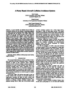
Figure 2. Type II (Medium)

Figure 3. Type III (Hard)

Using the subjective criterion of how perceivable objects are within the scene, there are 3 types of images: type I, II, and III. Visually type I corresponds to easily perceivable objects (see Figure 1), type II to medium (see Figure 2), and type III (see Figure 3) hard to perceive objects. The manual classification of our training dataset was done by 3 different subjects. Each subject was instructed to classify the image based on how easy was to perceive the wires in them. 2.2. Automatic image classification based on clutter The image classification used for this paper is based on the most commonly used clutter measure in the literature, which was proposed by Schmieder and Weathersby [8]. The measure is based on the intensity distribution by color at the pixel level.

µ= Where

1 N

N

∑(X

i

)

(1)

i =1

µ is the intensity mean, Xi is the individual pixel intensity, and N the total number of pixels.

σ=

N 1 (X i − µ)2 ∑ N ( N − 1) i =1

(2)

The clutter measure is given by average of the intensity variance of contiguous windows in the scene:

clutter =

1 K

K

∑σ

2 i

(3)

i =1

Where K represents the number of windows the image was divided into and described above.

σ

is the intensity standard deviation

3. WIRE DETECTION ALGORITHM The wire detection algorithm uses video information in order to detect thin lines. Consecutive frames are used to estimate relative motion of individual pixels in the scene, and then merge that information with an edge map produced by an edge detector. The feature map to be used consists of the detected edges with strength equal to their estimated motion. Next, the feature map is pre-processed in order to minimize the number of pixels to be further analyzed. The feature map is finally subdivided into 16 windows (4x4) and a Hough transform is performed in each of them. The resulting parameter space is tracked over time using a wire movement model [9], which predicts the next location of previously tracked wires, even when the wires themselves are not visible. This paper focuses on the area defined by the dashed boundary shown in the algorithm flowchart (see Figure 4), corresponding to the creation of the feature map to be processed.

Video

Frame Selection

Image Classification

Pre-Processing

Type

Feature Map

Motion Estimation

Wires I

II

III

Sub-Images

Parameter Selection Line Fitting

Tracking Model

Edge Detection

Figure 4. Algorithm flowchart

3.1. Edge detection and Motion estimation Edge detection is a fundamental operation in the detection process. A Canny edge detector [10] is used with dynamic parameter selection based on the clutter measure of the image. A challenging problem relies in the fact that most edge detectors, including Canny, do not make a distinction between edges of objects and edges originating from textured regions; consequently, cluttered backgrounds and image artifacts from low quality video, affect significantly the number of edges to be processed. Also, post-processing techniques will be affected by the performance of the edge detector, since the morphology of the connected components in the edge map will vary depending on the edge detector parameters. The edge detection process is robust against feature occlusion and objects in cluttered scenes, but its output is highly sensible to further-processing described in section 3.2; therefore, it is essential to optimize the edge detection combined with the pre-processing by using information about the visual complexity and quality of an image. Traditional methods to compute motion estimates using small masks based on the target size fail when trying to approximate motion values along thin lines, especially in cluttered backgrounds; therefore, a pixel level approach is necessary. Despite the fact that the optic flow and the motion field are not equal, in areas where the magnitude of the intensity gradient is large, it has been shown in [11] that the projection of the optic flow on the direction of the local intensity gradient is approximately equal to the normal flow; therefore, we estimate the relative average motion per pixel, by using the normal flow value at every pixel in the edge map. 3.2. The feature map and pre-processing It is important to perform data filtering strategies to speed up computations and alleviate the computational load on the Hough transform. We use an 8-connected component labeling on the edge map, to get a pixel count and discard small components. Using the detection performance on the training dataset, based on the cross product of the ground truth and the detected vectors, it is clear that components with a count of less than 50px do not carry any information that will affect significantly the detection process; thus, safely components with a pixel count less than 30px are eliminated. Non-linear shaped components are good candidates to be excluded from further processing; commonly, components with an eccentricity less than 0.98 are non-linear; however, lines in cluttered scenes or low quality video are often

connected with other components in the edge map. For the edge detection and pre-processing parameters training, the ratio of the number of edge pixels detected to the number of 8-connected components found is maximized. The Maximization criterion was chosen with 2 main purposes: (1) increase the vote count of true wires produced by the Hough transform (decreasing the possibility of miss detection and increasing the accuracy of the tracking process), and (2) decrease incidental alignment of components generated by clutter (decreasing the false alarm rate). Figure 5 shows the result of the parameter training using the entire training dataset, the peak of the surface represents the optimal parameter pair in the average for all images (σw, εw), where σw is Canny’s sigma and εw is the eccentricity threshold to be used during pre-processing.

Performance

100 80 60 40 20 0.60

Eccentricity

1

0.98

0.96

0.94

0.92

0.9

0

0.49 Sigma

Figure 5. Parameters training for all images

Without an automatic classification system the feature map for any image would have to be created by using (σw, εw), in which case complex scenes could be improperly processed generating poor detection results. By classifying a scene based on its clutter measure we get 3 pairs (σI, εI), (σII, εII), (σIII, εIII), which represent a viable parameter pair for each image type. Table 1 summarizes the results of the training and experimentation. Table 1. Parameters by image types

Image Type 1 2 3

Clutter Measure [0-30) [30-45) [45-70]

Sigma 0.61 0.61 0.58

Eccentricity 0.98 0.6 0.935

The final feature map is given by the merged output of the pre-processing techniques and pixels corresponding to high motion estimates. Since thin lines edges will be often 8-connected with other components in cluttered scenes, keeping high motion values is necessary to ensure that the closest lines in the scene will be kept.

4. DATASETS AND RESULTS The training dataset consists of 100 images, which were manually marked with their ground truth lines in order to be used as a performance measure for the edge detector and the pre-processing techniques. The objects present in the images are buildings, trees, power lines and wires. Images were taken under different weather (good weather, mist, and moderate rain) and lighting conditions (time of day). The test dataset has 16 videos (30fr/sec) with 1077 wires and 720x480px resolution. 4.1. Image classification results The automated classification system errors are summarized in Table 2. The errors are computed comparing the manual classification of the images discussed in section 2.1, to the classification obtained using the clutter measure. As depicted in Table 2, the clutter measure is sufficient to accurately classify type I and non-type I images, but the classification error

rate increases significantly for images with a clutter measure of greater than 45 units; this is, type III (hard) images are often (about 1 in 4) classified as type II (medium), which effectively increases the number of false alarms due to the low eccentricity threshold. In the other hand, type II images are most of the time correctly classified (about 9 in 10) making it possible for the algorithm to correctly detect wires that would not be possible otherwise. Clearly, low enough eccentricity thresholds could be used with the optimal sigma found during training, but this combination would not maximize the criterion ratio, increasing the false alarm rate and dramatically, reducing the overall usability of the algorithm. Table 2. Image classification on training dataset

Image Type Type I (Easy) Type II (Medium) Type III (Hard)

Clutter Measure [0-30) [30-45) [45-70]

Type 1 Error (α) 12% 20% 25%

Type 2 Error (β) 3% 12% 24%

Correct classification results are achieved on Figures 1-3. Figure 1 has a computed clutter measure of 22.4 (easy), Figure 2 of 32.1 (medium), and Figure 3 of 52.4 (hard). Classification of scenes where trees form a major part of the background proved to be more challenging than images where buildings are a major part of the background. The color distribution of trees is much different than buildings; the latest engulfs a much wither range of colors and bigger color differences than trees. Figures 6 (power lines in front of tress in rainy conditions) and 7 (thick wires in front of trees in foggy conditions) exemplify incorrect classification as less visually complex (hard type III images being classified as easy I) scenes due to low general contrast in the scenes. It is clear that bad weather conditions will significantly affect the clutter measure due to atmospheric scattering effects.

Figure 6. Clutter=25.1

Figure 7. Clutter=24.6

The biggest problem with the clutter measure it is based on the fact that it is computed by only using low level information (pixel intensities), and visual complexity is a high level concept based on human perception. Gestalt psychology proposes that perception as a whole is more than the sum of its parts; therefore, clutter measures that only take into consideration the pixel information are fundamentally flawed, and this is exemplified in Figures 8-9 as more complex scenes at the pixel level (see Figure 9) have a higher clutter measure than scenes more human-perceived complex scenes (see Figure 8).

Figure 8. Clutter=32.4

Figure 9. Clutter=38.7

4.2. Edge detection improvement Processing the feature map, eliminating components that correspond to clutter is essential in order to reduce the false alarm rate, but the number of true edges corresponding to wires is key in the detection process. Edge detection improvement is computed by using the ground truth wires in the training dataset, and the number of true edge pixels produced by the edge detection with automatic parameter selection. Figure 6 shows how using the maximization criterion directly improves the number of points to be fed to the Hough transform compared to the number of points that would be used with (σw, εw). Percentage Improvement

14 12 10 Easy

8

Medium 6

Hard

4 2 0

Image Difficulty Figure 10. Edge detection improvement

4.3. Wire detection results The results in Table 3 come from data gathered in controlled scenarios. However, using the global optimal parameters the algorithm was unable to handle real data without manual intervention (adjusting parameters manually), but the automatic classification system allows dynamic change of the algorithm parameters to accommodate for low contrast wires, dense clutter, or artifacts produced by low quality video. The data was collected in a search and rescue mission at hurricane Katrina in Pearlington, MS. The video sequence shows a SUAV that crashes into poor contrast power lines in a 60 frame video sequence (640x480px and 30fr/sec) severely affected by camera jitter, sensor noise, shadows, and video quality. During landing the pilot could not see the power lines in the display, and a crash occurred before 2 seconds after the lines started to appear in the display. The power lines are nearly invisible to the naked eye as shown in the sample frames in Figure 11. Adjusting parameters automatically, the detection rate for the first 16 frames is 25% (perhaps enough to save the aircraft), down from 56% if parameters are adjusted manually, which is a strong indication that internal algorithm parameters can be also adjusted based on the clutter measure of the window being processed. In the last 7 frames, the wires were always detected using manual parameters, and detected in 5 frames using automatic parameters. The last 7 frames of the video sequence represent the last moment of the flight, once the helicopter was getting closer to the power lines. Table 3. Detection performance on test dataset

Parameters Global Based on Image Complexity

Power Lines 1077 1077

False Positives 26% 35%

Detection 98% 94%

Figure 11. SUAV crashing against power lines

5. CONCLUSIONS Using a clutter measure an automated classification of images based on their visual complexity is achieved. The images are classified into 3 types: type I correspond to easily perceivable objects, type II to medium, and type III hard to perceive objects. The parameters for the creation of a feature map are adjusted according to the image type. The feature map is then used for further analysis in order to detect thin obstacles in the flight path of aircrafts, such as wires and power lines. Using the proposed classification system the edge detection process was improved by 5% and 12% for type II and III images respectively, compared to edge detection results using optimal parameters in the average for all image types. The system was able to detect thin wires in a poor quality 2 second crash sequence taken from a SUAV during hurricane Katrina, without any human intervention, effectively detecting low contrast power lines in video severely affected by camera jitter, sensor noise, shadows, and compression artifacts in 15% of the frames. Future papers will show how the clutter measure can be used within the detection process, in order to improve the detection as well as reduce the false alarm rate.

5. REFERENCES

[1] Rosenholtz, R., Li, Y., Mansfield, J., Jin, Z. “Feature congestion: a measure of display clutter” Proc. of the SIGCHI conference on Human factors in computing systems, 2005 [2] Avizonis, P., Barron, B. “Low cost wire detection system” Digital Avionics Systems Conference, 1999 [3]Gandhi, T., Yang M. T., Kasturi, R., Camps, O., Coraor, L., McCandless, J. “Detection of obstacles in the flight path of an aircraft” IEEE Trans. Aerospace and Electronic Systems, vol. 39, no. 1, pp. 176–191, 2003 [4] Yang, M. T., Gandhi, T., Kasturi, R., Coraor, L., Camps, O., McCandless, J. “Real-time obstacle detection system for high speed civil transport supersonic aircraft” Proc. of the National Aerospace and Electronics Conf, pp.595–601, 2000 [5] Arnold, J.; Shaw, S.W.; Pasternack, H.; “Efficient target tracking using dynamic programming” IEEE Trans. Aerospace and Electronic Systems, vol. 29, no. 1. pp. 44 – 56, 1993 [6] Barniv Y. “Dynamic programming solution for detecting dim moving targets,” IEEE Trans. Aerospace Electronic Systems, Vol. AES-21, no. 1, pp. 144-156, 1985 [7] Kasturi, R., Camps, O., Huang, Y., Narasimhamurthy, A., Pande, N. “Wire Detection Algorithms for Navigation”. Technical report, Dept. of CSE, The Pennsylvania State University, 2002 [8] Schmieder, E., and Weathersby, M. R. “Detection performance in clutter with variable resolution” IEEE Trans. Aerospace and Electronic Systems, AES-19, 1983 [9] Candamo, J., Kasturi, R., Goldgof, D., Sarkar, S., Jeanty, H. “Wire Detection in Low Quality Video” Technical Report. University of South Florida, Dec. 2005 [10] Canny, J. F. “A computational approach to edge detection” IEEE Trans. Pattern Anal. Machine Intell., vol. PAMI-8, no. 6, pp. 679–698, 1986 [11] Huang, L., Aloimonos, J. Y. “Relative depth from motion using normal flow: An active and purposive solution” Proc. IEEE Workshop on Visual Motion, 1991