Policy Compression for Aircraft Collision Avoidance Systems Kyle D. Julian∗ , Jessica Lopez† , Jeffrey S. Brush† , Michael P. Owen‡ and Mykel J. Kochenderfer∗ ∗ Department

of Aeronautics and Astronautics, Stanford University, Stanford, CA, 94305 Physics Laboratory, Johns Hopkins University, Laurel, MD, 20723 ‡ Lincoln Laboratory, Massachusetts Institute of Technology, Lexington, MA, 02420 † Applied

Abstract—One approach to designing the decision making logic for an aircraft collision avoidance system is to frame the problem as Markov decision process and optimize the system using dynamic programming. The resulting strategy can be represented as a numeric table. This methodology has been used in the development of the ACAS X family of collision avoidance systems for manned and unmanned aircraft. However, due to the high dimensionality of the state space, discretizing the state variables can lead to very large tables. To improve storage efficiency, we propose two approaches for compressing the lookup table. The first approach exploits redundancy in the table. The table is decomposed into a set of lower-dimensional tables, some of which can be represented by single tables in areas where the lowerdimensional tables are identical or nearly identical with respect to a similarity metric. The second approach uses a deep neural network to learn a complex non-linear function approximation of the table. With the use of an asymmetric loss function and a gradient descent algorithm, the parameters for this network can be trained to provide very accurate estimates of values while preserving the relative preferences of the possible advisories for each state. As a result, the table can be approximately represented by only the parameters of the network, which reduces the required storage space by a factor of 1000. Simulation studies show that system performance is very similar using either compressed table representation in place of the original table. Even though the neural network was trained directly on the original table, the network surpasses the original table on the performance metrics and encounter sets evaluated here.

I. I NTRODUCTION Decades of research have explored a variety of different approaches to designing the decision making logic for aircraft collision avoidance systems for both manned and unmanned aircraft [1]. Recent work on formulating the problem of collision avoidance as a partially observable Markov decision process (POMDP) has led to the development of the ACAS X family of collision avoidance systems [2], [3], [4]. The version for manned aircraft, ACAS Xa, is expected to become the next international standard for large commercial transport and cargo aircraft. The variant for unmanned aircraft, ACAS Xu, uses dynamic programming to determine horizontal or vertical resolution advisories in order to avoid collisions while minimizing disruptive alerts. ACAS Xu was successfully flight tested in 2014 using NASA’s Ikhana UAS [5]. The dynamic programming process for creating the ACAS Xu horizontal decision making logic results in a large numeric lookup table that contains scores associated with different maneuvers from millions of different discrete states. The table

is extremely large, requiring hundreds of gigabytes of floating point storage. A simple technique to reduce the size of the score table is to downsample the table after dynamic programming. To minimize the deterioration in decision quality, states are removed in areas where the variation between values in the table are smooth. This allows the table to be downsampled with only minor impact on overall decision performance. The downsampling reduces the size of the table by a factor of 180 from that produced by dynamic programming. For the rest of this paper, we refer to the downsampled ACAS Xu horizontal table as our baseline, original table. Even after downsampling, the current table requires over 2GB of floating point storage. Discretized score tables like this have been compressed with Gaussian processes [6] and decision trees [7]. For an earlier version of ACAS Xa, block compression was introduced to take advantage of the fact that, for many discrete states, the scores for the available actions are identical [8]. One critical contribution of that work was the observation that the table could be stored in IEEE half-precision with no appreciable loss of performance. Block compression was adequate for the ACAS Xa tables that limit advisories to vertical maneuvers, but the ACAS Xu tables are much larger. This paper explores two approaches for compressing the score table without loss of performance as measured by a set of safety and operational metrics. The first approach, origami compression, uses the natural symmetry present within the table to ‘fold’ the table by decomposing it into smaller tables and removing redundancies. With the use of a similarity metric to control the amount of tolerated loss during compression, the loss of fidelity of the compressed table can be chosen to yield a smaller size table that still provides acceptable performance. The second approach seeks to find a robust non-linear function approximation that represents the table. A deep neural network, which can serve as a robust global function approximator when trained using supervised learning, was used as the functional basis. Using an asymmetric loss function during training ensures that the approximated table is able to maintain the actions recommended by the original table while providing good estimates of the original score table values. This paper shows that both methods preserve the performance of the ACAS Xu system according to standard safety and operational performance metrics. These metrics are

evaluated using 1.5 million encounters with varied encounter geometries and sensor noise. Although the deep neural network reduces the required memory by a factor of 1000, it also improves the performance of the ACAS Xu system on the performance metrics evaluated in this paper. The neural network imposes regularity on the policy representation and smooths out artifacts from interpolation of the original discrete representation. Although there are significant certification concerns with neural network representations, which may be addressed in the future, these results indicate a promising way to compactly represent collision avoidance strategies without sacrificing performance. Section II provides an overview of the score table used in the ACAS Xu horizontal logic. Sections III and IV describe the two techniques used to compress the score table. Section V discusses performance results derived from the two forms of compressed score tables, and conclusions are presented in VI.

heading rates are defined as left turns and COC is represented by a 0 ◦ /s action. The optimal action to take from a given state can be extracted from the score table. If Q is the real-valued function associated with the eight-dimensional score table, then the optimal action is a∗ = arg max Q(ρ, θ, ψ, vown , vint , τ, aprev , a)

In general, the values of the state variables do not fall exactly on the grid points, in which case nearest-neighbor interpolation can be used. Since the surveillance sensors used by the aircraft are imperfect, there may be uncertainty in the current state measurement. To improve the robustness of the system to this uncertainty [9], ACAS Xu uses an unscented Kalman filter [10] to arrive at a set of weighted state-space samples. These weighted samples can then be used to compute the best action: a∗ = arg max b(s(i) )Q(s(i) , a)

II. S CORE TABLE

(2)

a

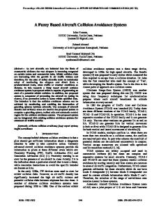
The ACAS Xu score table associates scores with all pairs of 120 million states and five actions. The state space is composed of seven dimensions, as shown in Fig. 1, which represent information that can be determined from sensor measurements [4]: 1) ρ (m): Distance from ownship to intruder. 2) θ (rad): Angle to intruder relative to ownship heading direction. 3) ψ (rad): Heading angle of intruder relative to ownship heading direction. 4) vown (m/s): Speed of ownship. 5) vint (m/s): Speed of intruder. 6) τ (sec): Time until loss of vertical separation. 7) aprev (◦ /s): Previous advisory.

ψ vint

(1)

a

Intruder

vown

where s(i) is the ith state sample and b(s(i) ) is its associated weight. III. O RIGAMI C OMPRESSION This section outlines the origami compression scheme used for reducing the size of the ACAS Xu table. A. Table Splitting The score table can be rearranged into a collection of smaller tables, one for each combination of previous action and current action. Since there are five possible actions, the original table can be split into 25 of these smaller tables (Q1 , . . . , Q25 ). Each of these tables is six dimensional. Inspection of the smaller tables revealed that there are patterns in the values that emerge from the process of dynamic programming. Similarities between many of the tables become apparent after subtracting out blocks in the score table related to the minimum scores across the τ dimension. Origami compression involves computing a set of 25 five-dimensional tables, where ¯ i (ρ, θ, ψ, vown , vint ) = min Qi (ρ, θ, ψ, vown , vint , τ ) Q τ

ρ

Origami looks for redundancy in the six-dimensional tables ¯ i is subtracted off of Qi . where Q ˜ i (ρ, θ, ψ, vown , vint , τ ) =Qi (ρ, θ, ψ, vown , vint , τ ) Q ¯ i (ρ, θ, ψ, vown , vint ) −Q

Ownship

θ Fig. 1. Geometry for ACAS Xu Horizontal Logic Table

The actions in the score table are the horizontal resolution advisories given to the ownship. These advisories tell the vehicle either it is Clear-of-Conflict (COC) or that it should turn left or right at one of two specified heading rates, 1.5 ◦ /s or 3.0 ◦ /s. Hence, there are five possible actions, where positive

(3)

(4)

B. Similarity Metric for Lossiness ˜1, . . . , Q ˜ 25 shows that many of the tables Inspection of Q are very similar. A similarity metric was used to group similar tables together into m equivalence classes, denoted ˜ (1) , . . . , Q ˜ (m) . Define the vector Q ˜i − Q ˜j | δij = |Q

(5)

˜ i and Q ˜ j in this context are treated as vectors where Q containing the values of the tables, and the absolute value

is applied element-wise to the vector. The distance between ˜ i and Q ˜ j is given by the scalar Q σij (ri + rj )/2

˜ (m) Q

(6)

where σij is the standard deviation of the elements in δij and ˜ i minus the minimum value of Q ˜i. ri the maximum value of Q ˜ i and For a given threshold level of tolerance , tables Q ˜ j can be grouped together when dij < . If  = 0, two Q splits must be exactly identical to be deemed equivalent. There is a tradeoff between loss (determined by ) and the overall size of the compressed score table. This tradeoff is discussed further in the results section in the context of overall system performance.

x2 ˜ (1) Q Input Variables ρ, θ, ψ, vown , vint τ aprev a

Eq. Class Table

Add score

¯i Q

C. Symmetry Exploitation Origami also searches for redundancies due to symmetry in the score table. Define the symmetric transformation reflecting about θ = 0 and ψ = 0 as: ˜ ∗ (ρ, θ, ψ, vown , vint , τ ) = Q ˜ i (ρ, −θ, −ψ, vown , vint , τ ) Q i

...

dij =

Set of m equivalence classes

Fig. 2. Origami Data Accessing Scheme

(7)

˜ i and Q ˜ ∗ when Inspection revealed similarities between Q j they correspond to combinations of aprev and a where the current actions are symmetric, i.e. left and right turns. After ˜i, Q ˜ j ) pairs, origami also computing dij for all possible (Q ˜i, Q ˜ ∗ ) pairs to identify computes the distance metric for all (Q j the additional symmetric equivalences. D. Data Layout The origami representation of the score table requires tracking auxiliary data for accessing the compressed scores in real time. As outlined in Fig. 2, we need to store: ˜ (1) , . . . , Q ˜ (m) , 1) m six-dimensional tables Q 2) a table mapping pairs of (aprev , a) to one of the m equivalence classes, and ¯1, . . . , Q ¯ 25 . 3) 25 five-dimensional offset tables Q This collection of auxiliary data can result in significant savings over storing the entire eight-dimensional score table. E. Implementation The origami folding algorithm is implemented in C++. Running on a current x64 based Windows machine, the algorithm required 55 seconds to read the 3.23 GB uncompressed data from (solid-state) disk, 25 seconds to identify the symmetries and equivalence classes, and 12 seconds to write the output files. While the algorithm is only implemented on a single thread, it is only the final two components that are amenable to parallelization. If the code was parallelized to take advantage of four cores, the total time to fold the table under study could be reduced from 92 seconds to 64 seconds. IV. D EEP N EURAL N ETWORK C OMPRESSION This section explains the development of a deep neural network function approximation of the score table.

A. Function Approximation Rather than storing all of the state-action scores explicitly, the values of the table can be represented as a non-linear, parametric function that takes as input the values of the state variables and outputs the scores of the various actions. Instead of storing the table itself, only the parameters of the function need to be stored, which could significantly decrease the amount of storage required to represent the table. Although the large size of the score table may make this approach seem intractable, recent advances in machine learning present a viable solution. Deep neural networks are large, non-linear functions that can be trained to approximate complex multidimensional target data [11]. A feed-forward neural network is composed of inputs that are weighted and summed into a layer of perceptrons. The value at each perceptron then passes through an activation function before being weighted and summed again to form the next layer of perceptrons. In a deep neural network, there are multiple layers, called hidden layers, before reaching the last layer, or output layer, which represents the function approximation for the score table. The weights and biases of the network can be trained so that a given set of inputs will accurately compute the score table values. The choices of the neural network architecture and features can help the network to train quickly and accurately. Figure 3 shows an example diagram of a fully-connected network with two hidden layers and rectified linear unit activations (ReLU) [12], which only allow positive inputs to pass through to the next layer. B. Model Architecture The deep neural network uses fully-connected feed-forward layers with ReLU activation after each hidden layer. The network has seven inputs, one for each of the seven state variables. The output layer consists of five output nodes, one for each possible advisory. With this architecture, one forward

Hidden Layer 2

Σ

Σ

Σ

Σ

Σ

Σ

Σ

Σ

10−2 Adadelta Adagrad AdaMax RMSprop Adam

Output Layer 10−3 Average Loss

Hidden Layer 1

Input Layer

10−4

10−5

10−6

Fig. 3. Neural Network Diagram

C. Loss Function Another important consideration in training the network to learn the score table is the choice of loss function to compute the error propagated back through the network to update the network parameters. For typical regression models, mean squared error (MSE) is used because it is simple,

50

100

150

200

250

300

10−4

Average Loss

pass through the network computes the cost values for each of the five advisories. Optimizing the network architecture can be challenging because there are many parameters to vary and evaluation of the different architectures can be slow. One important consideration in training deep neural networks is to select and tune the optimizer used to update the parameters and weights of the network. Different optimizers were evaluated including RMSprop [13], Adagrad [14], Adadelta [15], and Adam [16]. A variant of Adam, known as AdaMax [16], proved to learn the quickest without becoming stuck in local optima. In addition, AdaMax requires relatively little tuning of parameters because it uses estimates of the lower-order moments of the gradient to anneal the step size of the gradient descent [16]. After selecting AdaMax for the optimizer, different network architectures were investigated. A baseline architecture was chosen with five hidden layers and a set of layer sizes that is larger early in the network and tapers to smaller layer sizes towards the end of the network. This approach allows for the network to find increasingly more abstract representations of the data, similar to the approach with convolutional neural networks in image classification [11]. The layer sizes were also chosen so that the total number of parameters in the network would be around 600,000, as this would mean the table could be compressed to occupy only a few megabytes when using floating point precision. To test the baseline architecture, the number of hidden layers was varied to see the effect on the regression performance, but six hidden layers proved to give the best results with additional layers yielding little improvement. Figure 4 shows the network loss during training for the different network optimizers and number of layers. As a result of this study, a neural network with six hidden layers and AdaMax optimization was chosen.

0

3 4 5 6 7

HL HL HL HL HL

10−5

10−6

0

100

200

300

400

500

600

700

Number of Training Epochs Fig. 4. Training Comparisons

differentiable, and fast to compute. When applied to the problem of learning score table values, MSE gives accurate approximations. However, there is no longer a guarantee that the optimal advisory remains the same. For many of the states in the score table, the difference between the scores of the first and second best advisories is relatively small. When MSE fails to maintain the order of the actions, the network’s collision avoidance strategy can be very different from that of the original table. Predicting the optimal action given a set of inputs is a classification problem often solved with categorical cross entropy loss [17]. This approach can predict optimal actions well, but there is no regard for representing the score values. It is important to capture the score values too and not just the best action in order to accurately compute Eq. (2). To get the numeric accuracy of MSE with the classification accuracy of categorical cross entropy, an asymmetric version of MSE was used. Asymmetric loss functions have been used to train neural networks when positive or negative errors are not identical [18]. The asymmetric loss function for collision avoidance, shown in Fig. 5 is based on MSE, but it increases the penalty by a factor when the neural network over-estimates the cost of optimal advisories or under-estimates the cost of sub-optimal advisories. The factor applied to the optimal

advisory is four times greater than the suboptimal advisories to balance the fact that there are four sub-optimal advisories for every optimal advisory. With this loss function, the neural network has incentive to maintain the optimal advisories of the score table while still learning accurate representations of the table values.

Penalty for Error

Optimal Advisories Suboptimal Advisories

A. Performance 10 5 0 −1

−0.5

0

0.5

1

Cost Estimation Error Fig. 5. Asymmetric loss function penalties

The advantage of the asymmetric loss function over regular MSE can be visualized through the confusion matrices shown in Fig. 6. Each row is normalized to add up to 100% and represents the percentage of states where the neural network selected a particular advisory given the advisory of the original table. Asymmetric MSE Loss

Nominal MSE Loss Score Table Advisory

V. R ESULTS This section compares the two compression algorithms in terms of safety and operational performance in simulation, compression size, and run-time requirements.

20 15

each training epoch, the table data was shuffled and passed through the network in batches of 216 samples. We trained the network for 1,200 training epochs over the course of four days.

3

3

1.5

1.5

0

0

−1.5

−1.5

−3

−3

100% 80% 60% 40% 20%

−3−1.5 0 1.5 3

−3−1.5 0 1.5 3

Neural Network Advisory

Neural Network Advisory

0%

Fig. 6. Confusion matrices for MSE and asymmetric MSE loss

The entries on the main diagonal represent the percentage of advisories correctly classified by the neural network, while the off-diagonal entries show mis-classifications. For the turning advisories, the asymmetric loss function is much better at maintaining advisories and achieves on-diagonal percentages of 90–94% while the nominal MSE loss function maintains advisories only 72–74% of the time. D. Implementation We implemented the deep neural network in Python using the Keras library [19] running on top of Theano [20]. We trained the networks on an NVIDIA DIGITS DevBox with four Titan X GPUs. Before training, the score table was loaded as test data for the neural network. The inputs and table values were normalized so that each has a zero mean and range of one, which helps the network train more quickly [21]. For

One way to assess the quality of the compression is to plot the actions recommended by the original table and the compressed strategies for slices through the state space. These plots show top-down views of encounters with the ownship centered at the origin and flying in the direction indicated while the intruder vehicle is flying in the direction shown by the aircraft in the upper right corner of the plots. The color at each point in the plot shows the advisory the table would issue if the intruder were at that location. Figure 7 shows the actions for a head-on collision encounter with the aprev being COC. While the origami table with the lowest loss tolerance is almost identical to the original table, relaxing the loss tolerance begins to change the shape of the alerting regions. In addition, while the original and origami table plots appear choppy due to discretization and nearest neighbor interpolation, the neural network is able to produce regions that are smooth representations of the table. For the neural network, no interpolation is needed since raw input values can be passed directly to the neural network to compute the advisory costs of that state. The smoothing effect of the deep neural network representation can be seen for angled encounters as well. Figure 8 shows the policies for an aircraft approaching at a right angle with the previous advisory being −1.5 ◦ /s. The neural network shows a smooth representation of the table, while the origami tables show accurate representations of the original table. The origami table with the most loss consists of a single equivalence class - that is, a single policy to be applied across all previous advisories (and then adjusted according to the ¯ While this policy appears almost identical to contents of Q). the policy of the original table for τ = 0 and aprev = COC, when τ is increased, the policy diverges from the original. As seen in Fig. 9, when τ is set to a high value of 60 seconds, the strategy for this high loss table (which should be significantly different than the strategy for low τ , since the intruder aircraft is farther away vertically) remains the same as when τ = 0. The origami tables with more loss, those with small numbers of equivalence classes, essentially average the policies across aprev , which leads to the origami table alerting in situations that do not need alerts. Confusion matrices can again be used to show compression performance on an aggregate scale. Figure 10 shows the confusion matrices for three origami tables as well as the deep neural network. The origami representation with the smallest loss tolerance almost perfectly matches the original while

Origami:  = 0.0003

Crossrange (kft)

Original Table 10

10

5

5

5

0

0

0

−5

−5

−5

−10

0

10

20

30

−10

0

Origami:  = 0.003

Crossrange (kft)

Origami:  = 0.002

10

10

20

30

−10

Origami:  = 0.03 10

10

5

5

5

0

0

0

−5

−5

−5

0

10

20

30

−10

0

10

Downrange (kft)

20

30

−10

0

Downrange (kft)

Advisories:

−3.0 ◦ /s

COC

−1.5 ◦ /s

10

20

30

Neural Network

10

−10

0

10

20

30

Downrange (kft) 1.5 ◦ /s

3.0 ◦ /s

Fig. 7. Advisories for a head-on encounter with aprev = COC, τ = 0 s

Origami:  = 0.0003

Crossrange (kft)

Original Table 30

30

30

20

20

20

10

10

10

0

0 0

20

40

0 0

Origami:  = 0.003

Crossrange (kft)

Origami:  = 0.002

20

40

0

Origami:  = 0.03 30

30

20

20

20

10

10

10

0 0

20

40

0 0

Downrange (kft)

20

40

0

Downrange (kft)

Advisories:

COC

40

Neural Network

30

0

20

−3.0 ◦ /s

−1.5 ◦ /s

20 Downrange (kft)

1.5 ◦ /s

3.0 ◦ /s

Fig. 8. Advisories for a 90◦ encounter with aprev = −1.5 ◦ /s, τ = 0 s

40

Origami:  = 0.0003

Crossrange (kft)

Original Table 10

10

10

5

5

5

0

0

0

−5

−5

−5

−10

0

10

20

30

−10

0

Origami:  = 0.003

Crossrange (kft)

Origami:  = 0.002

10

20

30

−10

Origami:  = 0.03 10

10

5

5

5

0

0

0

−5

−5

−5

0

10

20

30

−10

0

Downrange (kft)

10

20

30

−10

0

Downrange (kft)

Advisories:

COC

−3.0 ◦ /s

−1.5 ◦ /s

10

20

30

Neural Network

10

−10

0

10

20

30

Downrange (kft) 1.5 ◦ /s

3.0 ◦ /s

Fig. 9. Advisories for a head-on encounter scenario with aprev = COC, τ = 60 s

Table Advisory

increasing the loss tolerance results in increasingly greater confusion. The neural network matches the original table actions well, though not as well as the lower loss tolerance origami tables. Origami Loss:  = 0.002

Origami Loss:  = 0.003

3

3

1.5

1.5

90% 80%

0

0

−1.5

−1.5

−3

−3

100%

70%

−3−1.5 0 1.5 3

−3−1.5 0 1.5 3

Origami Loss:  = 0.03

Neural Network

60% 50%

Table Advisory

40% 3

3

1.5

1.5

0

0

20%

−1.5

−1.5

10%

−3

−3

30%

−3−1.5 0 1.5 3

−3−1.5 0 1.5 3

Compressed Advisory

Compressed Advisory

0%

Fig. 10. Confusion matrices for different compression schemes

Similar to confusion matrices, analyzing differences between the action ordering of the original table and an alternative representation can help quantify the fidelity of that representation. These ordering difference metrics can be defined as the percentage of all discrete states for which the

TABLE I O RDER D IFFERENCES C OMPARISON Compression Origami:  = 0.0003 Origami:  = 0.002 Origami:  = 0.003 Origami:  = 0.03 Neural Network

Any Action

Best Two

Best

18.35% 18.59% 26.55% 26.81% 37.94%

7.33% 7.52% 13.69% 17.32% 23.83%

0.34% 0.36% 5.98% 11.61% 2.07%

relative ordering of the actions (when sorted by the cost associated with each of those actions) differs between the original table and the compressed representation for a subset of the actions. Table I shows three different ordering difference metrics for the origami tables and neural network. The first metric counts the percent of states where the ordering of any of the actions are switched, while the second metric counts only the states where the best two actions have changed, and the third counts only when the best action (with the lowest score) has changed. The neural network compression has many ordering differences when more than just the optimal action is considered, but it is still accurate when considering only the optimal action. The neural network was trained to maintain the optimal action at each state, but there is little incentive for the other actions to keep their order. The origami tables show more ordering differences as the loss tolerance increases. In addition to comparing how well advisory orders are maintained, the errors in the score values can show how well the compression performed. Similar to the policy plots shown above, Figure 11 shows a heat map for an encounter scenario, but Figure 11 shows the average error of the five advisory

TABLE II S IMULATION C OMPARISON Compression Original Table Origami:  = 0.0003 Origami:  = 0.002 Origami:  = 0.003 Origami:  = 0.03 Neural Network

TABLE III O RIGAMI S IZES

p(NMAC)

p(Alert)

p(Reversal)

1.546 × 10−4 1.545 × 10−4 1.545 × 10−4 1.296 × 10−4 1.554 × 10−4 1.272 × 10−4

0.55485 0.55499 0.55553 0.65317 0.62617 0.53128

0.007438 0.007447 0.007729 0.006794 0.011789 0.006903

scores rather than the value of the optimal advisory. For the neural network plot, only the discrete states are considered since we are comparing score values to the original table, which only contains values at discrete points. As expected, increasing the loss tolerance increases the magnitude of the score value errors. Unlike in the previous plots where the 0.002 loss tolerance tables looked identical to the the original score table, a very small difference has emerged, but it is not enough to affect the policy. The plots for higher loss origami tables are sensitive to changes in τ , just as seen in the policy plots. The plots shown here have a medium τ value of 20 seconds, but lower values will results in lower errors while higher values will result in higher errors for the origami tables with more loss. To quantify the performance of the compressed score representations against the performance of the original table, the neural network code was integrated into a framework for simulating aircraft encounters generated by an airspace encounter model [22]. Evaluating the performance metrics involved simulating over 1.5 million different encounter scenarios. Each encounter has a weight representing the relative probability of that scenario occurring. Table II compares the likelihood of different events including near mid-air collisions (NMACs), alerts, and advisory reversals (i.e., changing the direction of the advisory). For higher values of loss tolerance, the origami tables reduce the probability of collision by alerting more frequently. The neural network reduces all three metrics, performing even better than the original table. Figure 12 shows the ground tracks for a simulated encounter where the neural network yields a better outcome than the original table. The arrows perpendicular to the ownship paths show the turn advisories given by the original table and neural network. While both systems advise left turns, the neural network alerts sooner than the original table. This small change has a large impact as the encounter progresses. The aircraft following the table policy cannot avoid collision and switches advisory directions in an effort to pass behind the intruder, but this switch is too late and the encounter results in an NMAC. The neural network, in contrast, is able to turn to pass in front of the intruder and avoid collision. The switch in advisory at the end prevents the ownship from turning too much and colliding with the intruder. Because the neural network defines a continuous function with respect to the state variables, the neural network

Compression Origami: Origami: Origami: Origami:

 = 0.0003  = 0.002  = 0.003  = 0.03

Number of Eq. Classes

Table Size (MB)

15 8 7 1

812.6 492.6 446.9 172.7

sometimes extends the alerting region past areas where the nearest neighbor interpolation would give an alert. In cases like Figure 12, this small change propagates and makes the difference between colliding with or avoiding the intruder. On the other hand, although alerting earlier provides a safety benefit it often causes an increase in unnecessary alerts. While, the encounter set used throughout this paper is representative of encounters in the airspace, it is focused on evaluation of near-miss scenarios. Further analysis is necessary to determine if an alerting reduction still exists in encounter sets which include a broader sampling of encounter geometries. The ability to use continuous states may explain why the neural network is able to outperform the original score table on the encounter set used in this paper and could potentially enable similar performance in broader encounter sets as well. B. Storage Requirement Reduction The loss tolerance is a mechanism for directly controlling the tradeoff between size and fidelity of the origami table representation. Table I shows that the origami configuration with the lowest amount of loss preserves the optimal action in 99.66% of the table states. Table II illustrates that this high fidelity representation performs almost identically to the original table in simulation. As the loss tolerance increases, more loss is introduced into the origami representation and the original set of n splits is represented by fewer equivalence classes, as shown in Table III. This loss of fidelity results in deviations from the original score table in safety and alerting performance. The neural network occupies much less memory than the original table. When the weights are saved in a text file, the file occupies just 5MB. This file specifies 600,000 floats, which would occupy only 2.4MB in memory. Since the original table requires 600 million floats, the neural network compresses the table by a factor of 1000. C. Runtime Recovery of the cost for a set of inputs using the origami folding algorithm entails two interpolation operations along with two one-dimensional table accesses as shown in Section III-D. However, the fact that the multidimensional tables share all but one dimension in common allows us to efficiently compute the interpolants so that the runtime impact is not double what it would be with a single large table. Use of the origami folding technique slows the access by about 30% compared to direct table lookups [23].

Crossrange (kft)

Origami:  = 0.0003

Origami:  = 0.002

Origami:  = 0.003

10

10

10

0

0

0

−10

−10 0

20

40

−10 0

20

40

0

20

40

Downrange (kft) Origami:  = 0.03

Neural Network 5

10

4 3 0

0 2 1

−10

−10 0

20

40

0

20

Downrange (kft)

40

Average Error

Crossrange (kft)

10

0

Downrange (kft)

Fig. 11. Average Q errors for a head-on encounter with aprev = −1.5 ◦ /s, τ = 20 s

10

y (kft)

5

0

−5 Intruder Ownship: Table Ownship: Network

−10

−15 −15

−10

−5

0

5

x (kft) Fig. 12. Ground track comparison through simulation

Because the neural network must perform large matrix multiplications to compute the costs of each set of inputs, the neural network approach requires more time to operate. When tested on the NVIDIA DIGITS DevBox, the network calculations take 0.32 ms for each set of inputs, which is about 100 times slower than performing a table lookup. With the use of a BLAS library, which optimizes matrix operations for faster calculations, the computation time can be sped up to an average of 77 µs per set of inputs. VI. C ONCLUSION To decrease the size of the large score table used for ACAS Xu, two compression algorithms are introduced. Origami compression exploits redundancies and symmetries in the state and action spaces to compress the table with little loss. The

neural network compression finds a function approximation for the table that strives to maintain optimal advisories while approximating table values as well. Simulation shows that both compression algorithms perform as well as the original table. The origami approach gives a more accurate compression with faster runtime performance, while the neural network approach gives a smaller compressed representation at the expense of runtime speed. Although not explored in this paper, it is possible to use neural networks to compress the smaller tables associated with the equivalence classes produced by the origami approach. This may result in even higher quality compression. Future work will explore the effects of compressed tables on other aircraft encounter sets and surveillance sources. Additional investigations will incorporate coordinated actions for both the ownship and intruder, which will allow encounters between two or more aircraft with ACAS Xu to issue optimal advisories with knowledge of intruder aircrafts’ advisories [24]. In addition, the process of computing a score table, downsampling, and then training a neural network requires a large amount of time, making trade studies between different reward functions or dynamic models difficult. A future approach will incorporate deep reinforcement learning to learn a collision avoidance strategy while simultaneously training a neural network representation. This could greatly reduce the time to learn new collision avoidance strategies and lead to more accurate neural network models because the approach would not require any discretization. ACKNOWLEDGMENT The authors wish to thank Neal Suchy from the Federal Aviation Administration for his support. This paper has benefited from the work of Francois Chaubard as well as conversations

with Blake Wulfe. This work is sponsored by the Federal Aviation Administration under Air Force Contract #FA872105-C-002 and Volpe Contract #DTRT5715D30011. Opinions, interpretations, conclusions, and recommendations are those of the authors and are not necessarily endorsed by the United States Government.

[12]

[13]

R EFERENCES [1]

[2]

[3]

[4]

[5]

[6]

[7]

[8]

[9]

[10]

[11]

J. K. Kuchar and L. C. Yang, “A review of conflict detection and resolution modeling methods,” IEEE Transactions on Intelligent Transportation Systems, vol. 1, no. 4, pp. 179–189, 2000. M. J. Kochenderfer, “Optimized airborne collision avoidance,” in Decision Making under Uncertainty: Theory and Application, MIT Press, 2015. M. J. Kochenderfer, J. E. Holland, and J. P. Chryssanthacopoulos, “Next generation airborne collision avoidance system,” Lincoln Laboratory Journal, vol. 19, no. 1, pp. 17–33, 2012. M. J. Kochenderfer and J. P. Chryssanthacopoulos, “Robust airborne collision avoidance through dynamic programming,” Massachusetts Institute of Technology, Lincoln Laboratory, Project Report ATC-371, 2011. [Online]. Available: http : / / www. ll . mit . edu / mission / aviation / publications / publication - files / atc - reports / Kochenderfer 2011 ATC-371 WW-21458.pdf. M. Marston and G. Baca, “ACAS-Xu initial selfseparation flight tests,” NASA, Tech. Rep. DFRC-EDAA-TN22968, 2015. [Online]. Available: http://hdl. handle.net/2060/20150008347. Y. Engel, S. Mannor, and R. Meir, “Reinforcement learning with Gaussian processes,” in International Conference on Machine Learning (ICML), 2005. R. Munos and A. Moore, “Variable resolution discretization in optimal control,” Machine Learning, vol. 49, no. 2, pp. 291–323, 2002. M. J. Kochenderfer and N. Monath, “Compression of optimal value functions for Markov decision processes,” in Data Compression Conference, 2013. J. P. Chryssanthacopoulos and M. J. Kochenderfer, “Accounting for state uncertainty in collision avoidance,” AIAA Journal on Guidance, Control, and Dynamics, vol. 34, no. 4, pp. 951–960, 2011. S. Julier and J. Uhlmann, “Unscented filtering and nonlinear estimation,” Proceedings of the IEEE, vol. 92, no. 3, pp. 401–422, 2004. A. Krizhevsky, I. Sutskever, and G. E. Hinton, “Imagenet classification with deep convolutional neural networks,” in Advances in Neural Information Processing Systems (NIPS), 2012.

[14]

[15] [16] [17]

[18]

[19] [20]

[21]

[22]

[23]

[24]

G. E. Dahl, T. N. Sainath, and G. E. Hinton, “Improving deep neural networks for lvcsr using rectified linear units and dropout,” in International Conference on Acoustics, Speech, and Signal Processing (ICASSP), 2013. T. Tieleman and G. Hinton, “Lecture 6.5-rmsprop: Divide the gradient by a running average of its recent magnitude,” COURSERA: Neural Networks for Machine Learning, vol. 4, p. 2, 2012. J. Duchi, E. Hazan, and Y. Singer, “Adaptive subgradient methods for online learning and stochastic optimization,” Journal of Machine Learning, vol. 12, pp. 2121–2159, 2011. M. D. Zeiler. (2012). ADADELTA: an adaptive learning rate method. arXiv: 1212.5701. D. Kingma and J. Ba, “Adam: A method for stochastic optimization,” 2014. arXiv: 1412.6980. G. P. Zhang, “Neural networks for classification: A survey,” IEEE Transactions on Systems, Man, and Cybernetics, Part C: Applications and Reviews, vol. 30, no. 4, pp. 451–462, 2000. S. F. Crone, “Training artificial neural networks for time series prediction using asymmetric cost functions,” in International Conference on Neural Information Processing (ICONIP), vol. 5, 2002. F. Chollet. (2016). Keras: Deep learning library for Theano and TensorFlow, [Online]. Available: keras.io. Theano Development Team. (2016). Theano: A Python framework for fast computation of mathematical expressions. arXiv: 1605.02688. Y. A. LeCun, L. Bottou, G. B. Orr, and K.-R. M¨uller, “Efficient backprop,” in Neural Networks: Tricks of the Trade, G. Montavon, G. B. Orr, and K.-R. M¨uller, Eds., 2nd ed., Berlin: Springer, 2012, pp. 9–48. M. J. Kochenderfer, M. W. M. Edwards, L. P. Espindle, J. K. Kuchar, and J. D. Griffith, “Airspace encounter models for estimating collision risk,” AIAA Journal on Guidance, Control, and Dynamics, vol. 33, no. 2, pp. 487–499, 2010. R. W. Gardner and J. S. Brush, “Enabling real-time execution: Runtime-efficiency improvements for the next generation airborne collision avoidance algorithms,” in Digital Avionics Systems Conference (DASC), 2016. H. Y. Ong and M. J. Kochenderfer, “Short-term conflict resolution for unmanned aircraft traffic management,” in Digital Avionics Systems Conference (DASC), 2015.