Edward J. Hickin: River Hydraulics and Channel Form

Chapter 6

Sediment transport

Introduction Sediment transport modes in rivers Suspended-sediment transport Bedload transport Dissolved-load transport Suspended-sediment transport The physics of sediment suspension Fluid drag and settling velocity

The diffusion model of sediment suspension Direct measurement of suspended-sediment transport rate

Bedload Transport The physics of bed material transport Sediment entrainment

Measuring bedload transport rate Formulae for predicting bedload transport rate Bedforms Character Origins Role in sediment transport Total load measurements Sediment sources and sediment supply Drainage basin characteristics Supply-limited sediment transport The geography of sediment discharge from rivers

Introduction The discussion in the previous chapter assumes that the channel boundary is rigid and that the fluid moving through the channel is simply water. As we noted in Chapter 3, however, although there are such channels in nature, most are alluvial with deformable boundaries and they conduct much more than just water. Even at low discharges most natural rivers carry a complex fluid consisting of water and sediment of various kinds as well as organic litter and organisms, both dead and alive! Some of this material is carried near the channel boundary while some is carried within or on the surface of the flow; some is submerged, some floats and some is dissolved. Material moved by the flow, derived locally and from upstream sources, constitutes sediment transport. Some transported sediment may pass through a reach of channel with the flow as sediment throughput while some may be stored on the boundary for a period or residence time before moving on again. The relationship between the

Chapter 6: Sediment transport

boundary configuration and the flow in an alluvial channel is very complex and involves a discontinuous process of sediment exchange between the flow and the boundary. At certain times sediment will move mainly from the flow to the boundary, building up the bed and banks through the process we call deposition. At other times it will move mainly from the boundary to the flow through the process we call erosion. Short-term boundary adjustments (hours to days) are often termed cut and fill while longer-term changes (months to years) are termed degradation and aggradation. At still other times these sediment exchanges may be balanced, in which case the boundary will be stable and show no tendency to shift in position. Sediment transport modes in rivers Sediment is transported by the flow in one of three principal modes: as bedload transport, suspended-load transport or as dissolved-load transport. Although the dissolved load obviously is very important in sediment budget studies where interest, for example, might be in the total mass of material being exported from a river system, in the context of river geomorphology it is much less important than the particulate load. Some scientists find it useful to think in terms of an additional mode of transport, transitional between that moved as bedload and that forming the suspended load, called the saltation load. Although it will be convenient at times to use this term it does not represent a separate process; our focus here will be on suspended-load and bedload transport. Suspended-sediment transport refers to the particles or grains of sediment moved along a river within and wholly supported by the flow. In order for sediment grains to remain in suspension the upward-directed forces associated with turbulence in the flow must be strong enough to overcome the downward force of gravity acting on the grains. As physical reasoning implies, the suspended-sediment load consists largely of the finer fraction, the fine sand, silt and clay, of the sediment available to the river. Because turbulence is generated at the channel boundary and is most intense there, suspended sediment tends to have higher concentrations and involve coarser material near the boundary and both sediment size and concentration decline as we move up through the water column towards the surface of the flow. As we will see later, however, this general pattern can be distinctly modified in some rivers by the presence of sedimenttransporting flow structures such as vortices. In most rivers the bulk of transported sediment, often 90 per cent or more, moves as suspended-sediment load. The suspended load also includes the wash load of the flow. Wash load differs from the rest of the suspended load in that its suspension is not dependent on the forces of turbulence associated with flow. Rather it can be kept in suspension for a very long time by the fine-scale turbulence associated with molecular agitation (or Brownian motion) of the water. This motion continues even if the flow ceases as it might do where a river enters a slough or lake. The wash load is confined to the finest component (clay) of the available sediment. 6.2

Chapter 6: Sediment transport

Although the distinction here between bedload and suspended-sediment loads rests on fundamental differences in the physics of transport, it is important to keep in mind that any one grain size of sediment may at various times and places in the channel be transported in either of these modes. As the vigour of the flow increases, as it might through a channel contraction, a grain initially moving as bedload may become part of the suspended load where the turbulence intensity is elevated, and again return to the bed where the flow later expands and becomes more placid. Thus the mode of transport does not correspond in any precise way with a grain size. Sand may move as bedload in a small stream and as suspended-sediment load in a larger more vigorous river. Similarly, material found in the bed of a channel - the bed material - was not necessarily transported there as bedload nor does it define the size of material moved as bedload. If a wide range of grain sizes is available water surface to the flow some sediment will occupy a Flow direction transitional phase and may alternate between bedload and suspended load or may simply be intermittently suspended. Intermittent suspension, or saltation, river bed involves the disturbance of a grain on the bed (often caused by the impact of 6.1: The asymmetric trajectory of another grain) in such a way that it rises sediment grains in intermittent quickly and steeply into the flow to a suspension (saltation) peak height and then returns to the bed again at a slower rate. Thus the trajectory of such intermittently suspended grains in the flow is distinctively asymmetric (Figure 6.1). Bedload transport refers to the particles or grains of sediment moved along the bed of a river which are at all times wholly supported by the bed itself. In other words, bedload is bed material which moves by sliding and rolling, largely as a result of the shear stress exerted on the boundary by the flowing water. As you might expect, bedload consists largely of the coarser fraction, the sand and gravel, of the sediment available to the river. Bedload transport in many rivers commonly does not occur or is negligible at low flow, but as flow increases, the shear stress at the boundary eventually will exceed the threshold or critical conditions for bed particle movement and bedload transport will become active. At intermediate flows bedload transport often is confined to the thalweg of the channel (the locus of deepest flow along the channel) where the boundary shear stress is greatest. Bedload transport typically moves a small amount of sediment relative to the total sediment load and generally is less important than the suspended-load component in the context of sediment budgets. In gravel-bed rivers, for example, bedload commonly constitutes less than ten per cent of the total load. But as a geomorphic agent bedload transport exerts a fundamental control on the form and pattern of river channels and in this context is far more important than the suspended or dissolved sediment loads. 6.3

Chapter 6: Sediment transport

Dissolved load transport involves that component of the total load carried in solution. From a geomorphic perspective it is generally unimportant because it exerts little if any control over the form and pattern of the channel. Nevertheless, the total mass of material moved by rivers in this way can be a major component of the sediment budget of a drainage basin. It can be particularly significant in basins formed in highly soluble rocks such as limestones and marls. Indeed the geomorphology of karst landscapes, much of it below the surface of the ground, is primarily the product of dissolved load transported by surface and subterranean rivers. Suspended-sediment transport The physics of sediment suspension Fluid drag and settling velocity Sediment particles remain suspended in flowing water because the gravitational forces causing them to fall towards the bed are at times exceeded by the upward-acting lifting forces induced by the flow. In contrast, particles denser than water will always fall through standing water because the gravitational forces are unopposed by flow-induced lifting forces. Gravity will cause a particle to quickly accelerate towards the bed until the gravity force is opposed equally by the forces resisting movement, a state of balance in which the particle is said to have reached its terminal fall velocity or settling velocity. It will be very useful for us to consider the processes governing the settling velocity of sediment grains in standing water because the forces involved are at the heart of the suspension phenomenon. In much of the discussion to follow the sediment grains are considered to be spheres. This assumption is reasonable, because many natural particles in rivers do tend to be spherical, and convenient, because this simple symmetrical geometry allows us to more easily isolate the forces involved in settling. Later when we have the behaviour of spheres firmly pinned down we can relax this assumption and consider some of the complications introduced by less regular particle shapes. Meanwhile we must revisit some of the basic concepts of fluid deformation that we encountered in Chapter 5. The pattern of flow around settling spheres, shown in terms of streamlines in Figure 6.2, is of two basic types. In the first case, settling of the particle is controlled by the viscosity of the fluid and flow around the falling sphere is laminar. In the second, settling velocity of the particle is limited by inertial rather than viscous forces, and flow around the falling sphere is turbulent. The flow domains for these two settling conditions can be defined in terms of a particle Reynolds number (Rep) which is exactly analogous to the Reynolds number we considered earlier in Chapter 5. But in this context the characteristic length is not flow depth but rather is particle diameter (D) and flow velocity becomes the fall velocity (ω), thus:

6.4

Chapter 6: Sediment transport

inertial forces ωD Rep = viscous forces = .....................................(6.2) ν

When Rep < 0.1 grain settling is constrained overwhelmingly by viscous resistance. This condition is met only when the grains are small (in the silt-clay range; D1.0 is the state of entrainment. Similarly, once a particle has become entrained in the flow, whether or not transport is maintained depends on the ratio of transporting forces to resisting forces: Ct =

transporting forces ....................................................(6.25) resisting forces

Provided Ct in equation (6.1) remains at or above unity, the particle will remain in motion. Although equations (6.1) and (6.2) are conceptually identical they are operationally quite different because the entraining forces are not the same as the transporting forces (since the former is for a grain at rest and the latter is for one in motion) nor are the resisting forces identical in the two cases. For example, a grain may form part of an imbricated gravel bed, locked in place by neighbouring particles. In order to entrain the grain, sufficient force must be brought to bear on several particles in order to dislodge the grain from its resting place; less force is required to overcome the resisting forces once the grain is in motion. This circumstance is quite analogous to an aircraft which must expend greater energy (apply greater force) to overcome ground and air friction in order to become airborne than it does to overcome just air friction in order to stay aloft. Sediment entrainment, as noted above, occurs just beyond the threshold of motion at Ce = 1.0, when the entraining forces = resisting forces. Both sets of forces are very 6.15

Chapter 6: Sediment transport

complex, however, and the condition for the threshold defies analysis in all but the simplest cases. Nevertheless, it will be instructive to consider the forces involved qualitatively and to consider an analytical solution which at least illustrates the nature of the problem and provides the basis for some widely used semi-empirical models for defining the conditions for incipient motion . The entraining forces involve at least three groups of applied forces: • • •

impact force shear stress (drag force) lift forces (buoyancy, hydrodynamic lift, turbulence)

The impact force is the result of direct momentum transfer to the grain as the water impacts on the upstream-projected surface area. Actually, we have considered already the nature of the impact force in the context of the discussion of fall velocity. The impact force, Fi, for a single spherical grain at rest on a plane bed, is given by equation (6.3) if ω is replaced by the ambient velocity, v, striking the sphere:  π Fi = ρw v 2  D2 ..............................................................(6.26)  4

That is, the impact force is proportional to the flow velocity and grain diameter squared. Of course, equation (6.26) has no practical utility and its actual use would have to incorporate an empirical coefficient ( ϑ ) to at least allow for the effects of grain sheltering (degree of exposure to the oncoming flow), grain shape, and the fact that not all of the force of the directly impinging water is expended on the sphere ( Fi = ϕρwv 2D2 ). Shear stress is the tangential force exerted by the fluid as it flows over and around the grain on the bed. The unit force exerted on the sphere as the water shears over the channel boundary is given directly by equation (4.5). In a channel of rectangular crosssection the total shear stress applied to a single spherical particle on the bed (sometimes termed the tractive force) is given by the product of the shear stress term in equation (4.5) and the surface area of the sphere, thus: 2

τ o = ρw gdsϕπ D4

.........................................................(6.27)

where, again, ϕ is a coefficient reflecting the degree to which the sphere surface is exposed. Of course, if the shear stress were not uniformly distributed across the channel, a shear stress term such as that based on the local velocity distribution would be more appropriate than the depth/slope product (see Problem 5.3). The lift forces include the buoyant force, the hydrodynamic lift force, and the upward turbulence flux. The buoyant force is the hydrostatic force resulting from the particle/fluid density differences and is easily accounted for in the usual way as the buoyancy-discounted or submerged weight of the particle. The hydrodynamic lift force occurs because a grain on the bed is in the zone of steepest velocity gradient and the velocity at the base of the grain is considerably less than that at the top. In accordance with Bernoulli (which specifies an inverse relationship between velocity and pressure), 6.16

Chapter 6: Sediment transport

there is an upward declining pressure gradient which tends to lift the grain off the bed. The role of turbulence is not independent of the pressure-gradient force because excursions of velocity above the mean flow velocity obviously intensify that gradient temporarily and increase the lift at those times. But turbulence also involves other lifting forces, mostly not well understood. As water shears over the bed, turbulence is generated at the boundary in the form of wakes consisting of spinning parcels of water or vortices (eddies). These vortices move from the bed up into the flow, providing irregular upward pulses or bursts of high-velocity fluid motion. The upward force applied to bed particles by turbulence probably is the most important component of the lift force. Unfortunately it is also exceedingly complex and not amenable to any realistic analytical treatment. It is also very difficult to measure although several notable experimental studies (reviewed in Vanoni, 1975), suggest that the lift force can equal the drag force and exceed it by a factor of two or more in some flume flows. It has been argued that, because the lift forces involve the same basic variables as the drag force, the general expressions for both forces will have the same structure; see equation (6.12). The general lift equation for a spherical bed particle, therefore, becomes: FL =

CL k 2D2 ρ wv o 2 2

..............................................(6.28)

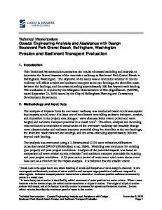
where CL is a lift coefficient (analogous to the drag coefficient), k2 is a particle shape factor, and Vo is flow velocity at the level of the particle. We might note that this relation only applies to fully turbulent flows (viscosity is omitted from consideration). This constraint is hardly limiting, however, since the viscous sublayer in all natural river flows would be completely disrupted by turbulence near the boundary. The relations among these competing forces is summarized in Figure 6.6A which shows a force diagram for roughly spherical particles resting on a river bed. Because the downstream slope of most channels is very small compared with the angle of repose of the grains in the bed we can assume that the mean bed surface is horizontal. The submerged weight or gravity force acts vertically downward through the centre of gravity of the grain and it is also subjected to the resultant of a horizontal drag force (or alternatively, an impact force) and a vertical lift force. Most analytical treatments of entraining forces acting on a grain on the bed consider only drag; lift does not appear explicitly. But it is argued that, because the resulting theoretical equations include coefficients of proportionality which are determined experimentally, and because lift depends on the same variables as drag, the effect of lift is automatically incorporated into the solutions. This may not seem like compelling reasoning to everyone but an alternative approach has yet to be offered and the assumption certainly is convenient and leads to some interesting and useful results. For example, if the incipient motion of the particle shown in Figure 6.6 involves rolling or rotating about a pivot point in the surface of easiest movement, the gravity and drag

6.17

Chapter 6: Sediment transport

forces can be resolved in that direction and the moments of the opposing forces can be equated to define the condition of incipient motion (see Figure 6.6B) as: FG sin α a1 = FD cos α a2 .............................................(6.29) where a1 and a2 are the unequal turning arms. The horizontal drag force FD in equation (6.29) is easily replaced by a more comprehensive resultant of both the lift forces and the drag force or by an alternative force such as the impact force. We will consider a couple of simple approaches but as we shall soon see, these analytical solutions have quite significant limitations and it is more useful to resort to a more general approach to the problem of defining incipient motion. It is not surprising that early thinking about incipient motion was in terms of flow velocity. The connection seemed so obvious that other factors influencing sediment motion were long neglected. We can derive an expression for incipient motion by solving equation (6.29) where the drag force is replaced by the impact force from equation (6.26) generalized to particles of projected area A ( Fi = ρw v 2A ). The gravity force exerted by a grain of volume, VO , is given by FG = Vo (ρs − ρ w )g. Thus, we can say that, at the point of incipient motion, the balance of moments is: Vo (ρ s − ρ w )gsineαa 1 = ρw v 2Aϑ cosαa 2

which can be simplified to

Vo  ρw   ϑ = A  ρ s − ρ w   tanα

a2  v 2 a 1  g

..........................………......(6.30)

in which ϑ is a coefficient of grain exposure. In the case of spheres, for which the 1 6

π 4

turning arms a1 and a2 are equal, Vo = πD3 and projected A = D 2 , equation (6.30) simplifies further to  ρ w   3 ϑ  v2 D=   ρ s − ρ w   2 tanα  g

6.18

........................................(6.31)

Lift component, FL

Chapter 6: Sediment transport

A Forces acting on a grain in the bed

, FF ce r fo

id Flu

Drag component, FD

C.G.

α

horizontal

mean bed surface

Dir mo ectio ve n o me f e nt as

ies

t

pivot

Gravity Force, FG FD cos α a2

B

α C.G.

Balance of moments for the drag component

a1

FD

α pivot

FG sine α

α FG

Movement begins when FG sine α a 1 = FD cos α a 2

6.6: (A) Forces acting on a grain resting on a bed of similar grains with a (B) balance of moments for the drag component at the onset of grain movement (After Middleton and Southard,1984).



ρ



3

ϑ 

The coefficients  w  and  will be sensibly constant for a particular sediment 2 tanα  ρ s − ρ w  mix and we can conclude that the diameter of particles barely moved by a stream varies with the square of the flow velocity: D ∝ v 2 . The cube of this proportionality, or D3 ∝ v 6 , implies that the mass, weight, or volume of a particle at the threshold of movement, varies with the sixth power of the flow velocity. It is perhaps surprising that this relationship, called the sixth power law (attributed to 6.19

Chapter 6: Sediment transport

Brahms, 1753) derived as it is for rather simple conditions, has been validated many times experimentally for particles coarser than about 2 mm in diameter. A particularly influential empirical study in this context is the analysis of erosion, transportation and deposition conducted by Hjulstrom (1935); his results are summarized in Figure 6.7. Hjulstromʼs entrainment criterion is a band in v-D space representing unconsolidated through consolidated sediment and has a general slope on this log/log plot that implies D ∝ v 2 in an approximate sense but only for grain sizes coarser than about 1 mm diameter. For grain sizes less than 0.1 mm diameter the entrainment velocity varies from a low of 6.7: Threshold velocities according to about 10 cms-1 for unconsolidated material Hjulstrom (1935) and transport and to almost 1000 cms-1 for consolidated bedform regimes (After Richards, 1982) material. The generally inverse relation between entrainment velocity and grain size less than 0.1 mm diameter reflects the fact that, as size declines in this range, increases in cohesive forces between the grains more than offset their declining mass. The lowest threshold mean velocity occurs for well-sorted 0.2-0.5 mm sands. The velocity criterion for deposition is less than that for entrainment (about two thirds) and is close to the fall velocity; the two converge closely for grains coarser than about 1.0 mm. Equation (6.29) can also provide a particular solution for sediment entrainment in terms of shear stress at the bed, a derivation first presented by White (1940). For spherical grains of the same diameter the submerged grain weight is FG = π number of grains per unit bed area is n = exposed area per grain is

D2 η

η D2

D3 (ρ − ρ w )g . 6 s

If the

, where η is a packing coefficient, the

so the total drag force FD =

τ oD2 η

.

Making these

substitutions in equation (6.29), and remembering that, for equal grain diameters the turning arms a1 = a2, yields for the condition of threshold movement: π

D3 τ D2 a1(ρ s − ρ w )g sin α = oc a 2 cos α 6 η

which can be simplified to: π τ oc = η (ρs − ρ w )gDtanα ........................................(6.31) 6

We might also note that τ oc π = η tanα ............................................(6.32) (ρ s − ρ w )gD 6 6.20

Chapter 6: Sediment transport

Equations (6.31) and (6.32) can be further modified to take account, for example, of a sloping bed, but they have no general practical use because of other limitations. For example, the influence of surrounding grains (such as imbrication) is ignored and the use of time-averaged measurements ignores the extreme transient stresses associated with turbulence. Equations (6.31) and (6.32) do provide, however, a theoretical framework for more general approaches. One such general approach to the problem of sediment entrainment was taken by Shields (1936) whose results are widely accepted and applied in solving river engineering problems.

6.8 (a): The Shields diagram as modified by Vanoni (1964) and (b): An extended Shields relation (larger range of Reynolds number/grain size) based on Miller et al, 1977 (from Allen, 1997).

6.21

Chapter 6: Sediment transport

Shields used experimental data to characterize, for a range of particle Reynolds number, the behaviour of the equilibrium force balance in a dimensionless critical shear stress term called the Shields criterion: θc =

τoc ....................................................(6.33) (ρ s − ρ w )gD

The structural similarity of equations (6.33) and (6.32) is quite apparent and reveals the physical basis of the Shields entrainment function which is graphed in Figure 6.8. For small Reynolds number (Rep