Chapter 3
Noncohesive Sediment Transport Page 3.1 Introduction .......................................................................................................................... 3-1 3.2 Incipient Motion ...................................................................................................................3-1 3.2.1 Shear Stress Approach .............................................................................................. 3-2 3.2.2 Velocity Approach ....................................................................................................3-7 3.3 Sediment Transport Functions ...........................................................................................3-12 3.3.1 Regime Approach ............................................................................................... 3-12 3.3.2 Regression Approach ..............................................................................................3-14 3.3.3 Probabilistic Approach .......................................................................................... 3-16 3.3.4 Deterministic Approach ..........................................................................................3-17 3 3.5 Stream Power Approach.......................................................................................... 3-23 3.3.5.1 Bagnold's Approach ................................................................................. 3-23 3.3.5.2 Engelund and Hansen's Approach ...........................................................3-25 3.3.5.3 Ackers and White's Approach .................................................................3-25 3.3.6 Unit Stream Power Approach .................................................................................3-28 3.3.7 Power Balance Approach ........................................................................................ 3-32 3.3.8 Gravitational Power Approach ................................................................................3-34 3.4 Other Commonly Used Sediment Transport Functions...................................................... 3-36 3.4.1 Schoklitsch Bedload Formula ................................................................................. 3-36 3.4.2 Kalinske BedloadFormula ..................................................................................3-37 3.4.3 Meyer-Peter and Miiller Formula ............................................................................ 3-39 3.4.4 Rottner Bedload Formula ........................................................................................3-40 3.4.5 Einstein Bedload Formula ....................................................................................... 3-41 3.4.6 Laursen Bed-Material Load Formula .................................................................... 3-41 3.4.7 Colby Bed-Material Load Formula .........................................................................3-42 3.4.8 Einstein Bed-Material Load Formula .................................................................... 3-44 3.4.9 Toffaleti Formula ....................................................................................................3-44 3.5 Fall Velocity ....................................................................................................................... 3-45 3.6 Resistance to Flow .............................................................................................................3-47 3.6.1 Einstein's Method ...................................................................................................3-49 3.6.2 Engelund and Hansen's Method ............................................................................. 3-54 3-58 3.6.3 Yang's Method ................................................................................................... 3.7 Nonequilibrium Sediment Transport .................................................................................. 3-63 3.8 Comparison and Selection of Sediment Transport Formulas .............................................3-63 3.8.1 Direct Comparisons with Measurements................................................................. 3-64 3.8.2 Comparison by Size Fraction .................................................................................. 3-73 3.8.3 Computer Model Simulation Comparison ...............................................................3-77 3.8.4 Selection of Sediment Transport Formulas ........................................................... 3-83 3.8.4.1 Dimensionless Parameters ........................................................................3-85 3.8.4.2 Data Analysis ........................................................................................... 3-86 3.8.4.3 Procedures for Selecting Sediment Transport Formulas ......................... 3-102 3- 104 3.9 Summary .......................................................................................................................... 3.10 References ........................................................................................................................ 3- 104
Chapter 3
Noncohesive Sediment Transport by Chih Ted Yang
3.1 Introduction Engineers, geologists, and river morphologists have studied the subject of sediment transport for centuries. Different approaches have been used for the development of sediment transport functions or formulas. These formulas have been used for solving engineering and environmental problems. Results obtained from different approaches often differ drastically from each other and from observations in the field. Some of the basic concepts, their limits of application, and the interrelationships among them have become clear to us only in recent years. Many of the complex aspects of sediment transport are yet to be understood, and they remain among the challenging subjects for future studies. The mechanics of sediment transport for cohesive and noncohesive materials are different. Issues relating to cohesive sediment transport will be addressed in chapter 4. This chapter addresses noncohesive sediment transport only. This chapter starts with a review of the basic concepts and approaches used in the derivation of incipient motion criteria and sediment transport functions or formulas. Evaluations and comparisons of some of the commonly used criteria and transport functions give readers general guidance on the selection of proper functions under different flow and sediment conditions. Some of the materials summarized in this chapter can be found in the book Sediment Transport Theory and Pmctice (Yang, 1996). Most noncohesive sediment transport formulas were developed for sediment transport in clear water under equilibrium conditions. Understanding sediment transport in sediment-laden flows with a high concentration of wash load is necessary for solving practical engineering problems. The need to consider nonequilibrium sediment transport in a sediment routing model is also addressed in this chapter.
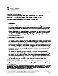
3.2 Incipient Motion Incipient motion is important in the study of sediment transport, channel degradation, and stable channel design. Due to the stochastic nature of sediment movement along an alluvial bed, it is difficult to define precisely at what flow condition a sediment particle will begin to move. Consequently, it depends more or less on an investigator's definition of incipient motion. They use terms such as "initial motion," "several grain moving," "weak movement," and "critical movement.!' In spite of these differences in definition, significant progress has been made on the study of incipient motion, both theoretically and experimentally. Figure 3.1 shows the forces acting on a spherical sediment particle at the bottom of an open channel. For most natural rivers, the channel slopes are small enough that the component of gravitational force in the direction of flow can be neglected compared with other forces acting on a spherical sediment particle. The forces to be considered are the drag force FD, lift force FL, submerged weight W,y,and resistance force FR. A sediment particle is at a state of incipient motion when one of the following conditions is satisfied:
Err~sionand Secimerzt~itionManual
w 3
Figure 3.1. Diagram of forces acting on a sediment particle in open channel tlow (Yang, 1973).
where
Mo = overturning moment due to FD and FL, and MR = resisting moment due to FL and W,.
Most incipient motion criteria are derived from either a shear stress or a velocity approach.
3.2.1 Shear Stress Approach One of the most prominent and widely used incipient motion criteria is the Shields diagram (1936) based on shear stress. Shields assumed that the factors in the determination of incipient motion are the shear stress r, the difference in density between sediment and fluidp, - p+, the diameter of the particle d, the kinematic viscosity v, and the gravitational acceleration g. These five quantities can be grouped into two dimensionless quantities, namely,
and
Chclpter 3-Noncohesive Sedirnenf Transport where
p , and pf y
= densities of sediment and fluid, respectively,
= specific weight of water, U:.: = shear velocity, and t,. = critical shear stress at initial motion.
The relationship between these two parameters is then determined experimentally. Figure 3.2 shows the experimental results obtained by Shields and other investigators at incipient motion. At points above the curve, the particle will move. At points below the curve, the flow is unable to move the particle. It should be pointed out that Shields did not fit a curve to the data but showed a band of considerable width. Rouse (1 939) first proposed the curve shown in Figure 3.2. Although engineers have used the Shields diagram widely as a criterion for incipient motion, dissatisfactions can be found in the literature. Yang (1973) pointed out the following factors and suggested that the Shields' diagram may not be the most desirable criterion for incipient motion.
x,
< I
1.00 0.80 0.60
x Sand (U.S. WES) A Sand (Gilbert)
j 2, f
0.30
g
0.20
2.65
2.65
Sand in air (White)
2.10
9,
a
.P
.j ::;
0.06 0.05 0.04 0.03 0.2
0.4 0.6 1.0
2
4
6 8 10
20
40
60 100
200
500
1000
I
Boundary Reynolds number U*d/v
F i g ~ ~3.2. r e Shields diagram Sor incipient motion (Vanoni. 1975)
The justification for selecting shear stress instead of average flow velocity is based on the existence of a universal velocity distribution law that facilitates computation of the shear stress from shear velocity and fluid density. Theoretically, water depth does not appear to be related directly to the shear stress calculation, while the main velocity is a function of water depth. However, in common practice, the shear stress is replaced by the average shear stress or tractive force t = yDS,where 11 is the specific weight of water, D is the water depth, and S is the energy slope. In this case, the average shear stress depends on the water depth. Although by assuming the existence of a universal velocity distribution law, the shear velocity or shear stress is a measure of the intensity of turbulent fluctuations, our present knowledge of turbulence is limited mainly to laboratory studies.
Erosion and Sedimentation Manual
•
Shields derived his criterion for incipient motion by using the concept of a laminar sublayer, according to which the laminar sublayer should not have any effect on the velocity distribution when the shear velocity Reynolds number is greater than 70. However, the Shields diagram clearly indicates that his dimensionless critical shear stress still varies with shear velocity Reynolds number when the latter is greater than 70.
•
Shields extends his curve to a straight line when the shear velocity Reynolds number is less than three. This means that when the sediment particle is very small, the critical tractive force is independent of sediment size (Liu, 1958). However, White (1940) showed that for a small shear velocity Reynolds number, the critical tractive force is proportional to the sediment size.
•
It is not appropriate to use both shear stress τ and shear velocity U* in the Shields diagram as dependent and independent variables because they are interchangeable by U* = (τ /ρ)1/2, where ρ is the fluid density. Consequently, the critical shear stress cannot be determined directly from Shields= diagram; it must be determined through trial and error.
•
Shields simplified the problem by neglecting the lift force and considering only the drag force. The lift force cannot be neglected, especially at high shear velocity Reynolds numbers.
•
Because the rate of sediment transport cannot be uniquely determined by shear stress (Brooks, 1955; Yang, 1972), it is questionable whether critical shear stress should be used as the criterion for incipient motion of sediment transport.
One of the objections to the use of the Shields diagram is that the dependent variables appear in both ordinate and abscissa parameters. Depending on the nature of the problem, the dependent variable can be critical shear stress or grain size. The American Society of Civil Engineers Task Committee on the Preparation of a Sediment manual (Vanoni, 1977) uses a third parameter
d v
1/ 2
⎡ ⎛ γs ⎞ ⎤ ⎢0.1 ⎜ − 1⎟ gd ⎥ ⎠ ⎦ ⎣ ⎝γ
as shown in Figure 3.2. The use of this parameter enables us to determine its intersection with the Shields diagram and its corresponding values of shear stress. The basic relationship shown in Figure 3.2 has been tested and modified by different investigators. Figure 3.3 shows the results summarized by Govers (1987) in accordance with a modified Shields diagram suggested by Yalin and Karahan (1979).
3-4
Chcq~ter3-Noncohesive Sediment Transport 6.00 4.00
-
I
I
I I I
I
I
I I I
I
Explanation: r White, C.M.(1940) w White, S.J.(1970) x Yalin and Karahan A Govers (1987) rn Govers (1987)
L-
I
I I I
I
I
I I I
I
I
-
Laminar flow Turbulent flow
Modified Shields curve (Yalin and Kmahan, 1979)
Shear velocity Reynolds number U.dh Figure 3.3. Modified Shields diagram (Govers, 1987)
Bureau of Reclamation (1 987) developed some stable channel design criteria based on the critical shear stress required to move sediment particles in channels under different flow and sediment conditions. The critical tractive force can be expressed by:
where
.s,
y D
= critical tractive force or shear stress (in lb/ft2 or g/m'), = specific weight of water (= 62.4 lblft' or 1 ton/m3), and = mean flow depth (in ft or m).
Figure 3.4 shows the relationship between critical tractive force and mean sediment diameter for stable channel design recommended by Bureau of Reclamation (1 977). Lane ( 1 953) developed stable channel design curves for trapezoidal channels with different typical side slopes. These curves are based on maximum allowable tractive force and are shown in Figure 3.5. Figure 3.5(a) is for the channel sides, and Figure 3.5(b) is for the channel bottom. Figure 3.5 indicates that the maximum shear stress is about equal to yDS and 0.75yDS for the bottom and the sides of the channel, respectively. Lane's study also shows that shear stress is zero at the corners. The shear stress acting on the channel side at incipient motion is:
Err~sionand Secimerzt~itionManual
Mean diameter (mm)
Figure 3.4. Tractive force versus transportable sediment size (Bureau of Reclamation, 1987).
Chclpter 3-Noncohesive Sedirnenf Transport
Figure 3.6. Erosion-deposition criteria for uniform particles (Hjulstrom, 1935).
At the bottom of a channel, 8 = 0, and equation (3.7) becomes:
z,= W, tan 4 The ratio of limiting tractive forces acting on the channel side and channel bottom is:
For stable channel design, the value of th can be obtained from the Shields diagram as shown in Figure 3.2, or from Figure 3.4 for channels of different materials.
3.2.2 Velocity Approach Fortier and Scobey (1 926) made an extensive field survey of maximum permissible values of mean velocity in canals. Table 3.1 shows their permissible velocities for canals of different materials. Hjulstrom (1935) made detailed analyses of the movement of uniform materials on the bottom of channels. Figure 3.6 gives the relationship between sediment size and average flow velocity for erosion, transportation, and sedimentation. The American Society of Civil Engineers Sedimentation Task Committee (Vanoni, 1977) suggested the use of Figure 3.7 for stable channel design.
Err~sionand Secimerzt(ition Manual
Table 3.1 Permissible canal velocities (Fortier and Scobey. 1926) Velocity* (CLIs)
Original matcrial excavated for canal (1) Fine sand (noncolloidal) Sandy loam (noncolloidal) Silt loam (noncolloidal) Alluvial sills when noncolloidal Ordinary firm loam Volcanic ash Fine gravel Stiff clay (very colloidal) Graded, loam to cobbles, when noncolloidal Alluvial silts when colloidal Graded, silt to cobbles, when colloidal Coarse gravel (noncolloidal) Cobbles and shingles Shales and hard ~ a n s
Clcar watcr, no detritus (2)
Water transporting colloidal sills (3)
Watcr transporting noncolloidal silts, sands, gravcls, or rock Pragmen ts (4)
1 .SO 1.75 2.00 2.00 2.50 2.50 2.50 3.75 3.75 3.75 4.00 4.00 5.00 6.00
2.50 2.50 3.00 3.50 3.50 3.50 5.00 5.00 5.00 5.00 5.50 6.00 5.50 6.00
1 .SO 2.00 2.00 2.00 2.25 2.00 7.75 3.00 5.00 3.00 5.00 6.50 6.50 5.00
''; For channels with depth of 3 ft or less after aging
Mean sediment size (mm)
Figurc 3.7. Critical watcr vclocitics for quart7 scdimcnt as a fi~nctionof mean grain s i x (Vanoni, 1977).
Yang ( 1 973) applied some basic theories in fluid mechanics to develop his incipient motion criteria. At incipient motion, the resistance force FR in Figure 3.1 should be balanced by the drag force FD. It can be shown that:
Chczpter 3LNoncohesive Sedi~nenfTransport The lift force acting on the particle can be obtained as:
The submerged weight of the particle is:
The resistant force:
where
y/,,
yz,y3 = coefficients, p, p.7 = density of water and sediment, respectively, D = average flow depth, D = sediment particle diameter, cc, = sediment particle fall velocity, V = average flow velocity, and B = roughness function.
Assume that the incipient motion occurs when FD = FR. From equations (3.10) and (3.13):
where
V,., = average critical velocity at incipient motion, and V,,/co = dimensionless critical velocity.
In the hydraulically smooth regime, B is a function of only the shear velocity Reynolds number U.:dv, that is,
where
U . = shear velocity, and v = kinematic viscosity of water.
Err~sionand Secimerzt~itionManual Then equation (3.14) becomes:
which is a hyperbola on a semilog plot between V,.,/oand U;.d/v. The relative roughness d/D should not have any significant influence on the shape of this hyperbola in the hydraulically smooth regime. In the completely rough regime, the laminar friction contribution can be neglected, andB is a function of only the relative roughness d/D, that is: B = 8.5,
U.,d ->70 v
Then equation (3.14) becomes:
Equation (3.18) indicates that in the completely rough regime, the plot of V,.,/o against U.[.cl/vis a straight horizontal line. The position of this horizontal line depends on the value of the relative roughness, y , , y2,and y3. In the transition regime with the shear velocity Reynolds number between 5 and 70, protrusions extend partly outside the laminar sublayer. Both the laminar friction and turbulent friction contributions should be considered. In this case, B deviates gradually from equation (3.15) with increasing U+dv.It is reasonable to expect that, basically, equation (3.16) is still valid, but with the relative roughness d D playing an increasingly important role as U d v increases. Yang (1973) used laboratory data collected by different investigators for the determination of coefficients in equations (3.16) and (3.18). The incipient motion criteria thus obtained are:
and
Chclpter 3-Noncohesive Sedirnenf Transport 28 26
I
I
1 1 1 1 111
I
1
1 111111
1
I
I
1 l Ill
Explanation:
-
0
-
Casey
V Grand Laboratory A Gilbert
24 -
-
Kramer m Th1jsse V Tison A Vanoni a U.S. Waterways Experiment Station 0
22
-
-
20-
?
18-
-
bU
b
'g a
3
B
'E
16
-
-
--
14 -
f.-
12-
3
10-
Transition -Compktely
rough
I I
7
-
I
I I I
E
-
I
I I I
8
-
smooth-
YJ
-
-
I I I
I
6
-
"a -
2'5
+0.66
log (U.d/v)- 0.06
-
I
I I
4-
I
4 A
v
2-
0
I O1
I
1 1 1 1 111 10
I
1
V Av
1 111111 100
v
I
A
I
I I I IIL
loo0
Shear velocity Reynolds number Re = U . d h
Figirrc 3.8. Relationship hctwccn dirncnsionlcss critical average velocity and Rcynolds numhcr (Yang, 1973). 30 0
.3
25
Explanation: o Govers (1987) (laminar flow) Talapatra and Ghosh (1983) (turbulent flow)
c
-
C
>=
$ 20-
-
d
1
2
5
10
20
50
100
200
500
loo0
Shear velocity Reynolds number Re = U.dlv
Figure 3.9. Verification of Yang's incipient motion criteria (Yang, 1996, 2003).
Err~sionand Secimerzt~itionManual Equation (3.19) indicates that the relationship between dimensionless critical average flow velocity and Reynolds number follows a hyperbola when the Reynolds number is less than 70. When the Reynolds number is greater than 70, V,,/w becomes a constant, as shown in equation (3.20). Figure 3.8 shows comparisons between equations (3.19), (3.20), and laboratory data. Figure 3.9 summarizes independent laboratory verification of Yang's criteria by Govers (1987) and Talapatra and Ghosh ( 1983).
3.3 Sediment Transport Functions The basic approaches used in the derivation of sediment transport functions or formulas are the regime, regression, probabilistic, and deterministic approaches. The basic assumptions, their limits of applications, and the theoretical basis of the above approaches and some of the more recent approaches based on the power concept are summarized herein.
3.3.1 Regime Approach A regime channel is an alluvial channel in dynamic equilibrium without noticeable long-term aggradations, degradation, or change of channel geometry and profile. Some site-specificquantitative relationships exist among sediment transport rates or concentration, hydraulic parameters, and channel geometry parameters. The so-called "regime theory1'or "regime equations" are empirical results based on long-term observations of stable canals in India and Pakistan. Blench (1 969) summarizes the range of regime channel data as shown in Table 3.2. The regime equations obtained from the regime concept are mainly obtained from the regression analysis of regime canal data.
Different sets of regime equations have been proposed by different investigators, such as those by Blench ( I 969), Kennedy (1 895), and Lacy ( 1 929). According to Blench, applications of regime equations have the following limitations: Steady discharge. Steady bed-sediment discharges of too small an amount to appear explicitly in the equations. Duned sand bed with the particle size distribution natural in the sense of following lognormal distribution. Suspended load insufficient to affect the equations. Steep, cohesive sides that are erodible or depositable from suspension and behave as hydraulically smooth. Straightness in the plan, so that the smoothed, duned bed is level across the cross-section. Uniform section and slope.
Chclpter 3-Noncohesive Sedirnenf Transport Constant water viscosity. Range of important parameters as shown in Table 3.2 or in whatever extrapolated range permits the same phase of flow. Table 3.2 Regime canal data range (after Blench, 1969) Particle size d. m m Silt grading Concentration pcr I pi Suspcndcd load Watcr tcinpcraturc Channel sides material Width-depth ratio, B/D v2/n,n/s2 VB/v Water discharge, Q, ft3/s Bed form D/d
0.10-0.60 log probability 0 to about 3 0- I %J 50-86 O F clay, smooth 4-30 0.5- 1 ,S 1 0"- 1ox 1 - 10,000 dunes > 1,000
Specifically, the equations are unlikely to apply if the width-depth ratio falls below about 5, or the depth below about 400 millimeters. The channel-forming discharge, or the dominant discharge, and sediment load or silt factors are the two most important factors to be considered in regime equations. The regime equations are useful engineering tools for stable canal design, especially for those in Pakistan and India. However, they have been subject to criticism for their lack of rational and physical rigor. No regime equations are given in this chapter. Readers who are interested in the application of regime equations should study the conditions under which these empirical equations were obtained. Applications of regime equations to conditions outside of the range of data used in deriving them could lead to erroneous results. The concept of "regime" is similar to the concepts of "dynamic equilibrium" and "hydraulic geometry." Lacy's (1 929) regime equation describing the relationships among channel slope S, water discharge Q, and silt fact0r.L for sediment transport is:
Leopold and Maddock's (1 953) hydraulic geometry relationships are:
Err~sionand Secimerzt~itionManual where
W D V Q
a, b, c, j k, m
= channel width,
channel depth, = average flow velocity, = water discharge, and = site-specific constants. =
Yang, et al. (1 98 1) applied the unit stream power theory for sediment transport (Yang, 1973), the theory of minimum unit stream power (Yang, 1971, 1976; Yang and Song, 1979, 1986), and the hydraulic geometry relationships shown in equations (3.22) through (3.24) to derive the relationship between Q and S. They also assumed that:
where
i, j = constants.
The theoretically derived j value is -2111, which is very close to the empirical value of equation (3.21).
-116
shown in
3.3.2 Regression Approach Some researchers believe that sediment transport is such a complex phenomenon that no single hydraulic parameter or combination of parameters can be found to describe sediment transport rate under all conditions. Instead of trying to find a dominant variable that can determine the rate of sediment transport, they recommend the use of regressions based on laboratory and field data. The parameters used in these regression equations may or may not have any physical meaning relating to the mechanics of sediment transport. Shen and Hung (1972) proposed the following regression equation based on 587 sets of laboratory data in the sand size range: log C, = -107,404.459381 64 + 324,214.74734085Y -326,309.58908739Y2+ 109,503.87232539Y3
where
y
=
C,
= total sediment concentration in ppm by weight, and = average fall velocity of sediment particles.
w
(3.26)
(VS0.57/W0.3210.007'0189
Before equation (3.26) was finally adopted by Shen and Hung, they performed a sensitivity analysis on the importance of different variables to the rate of sediment transport. Because laboratory data have limited range of variation of water depth, the sensitivity analysis indicated that the rate of sediment transport was not sensitive to changes in water depth. Consequently, water depth was eliminated from consideration. The dimensionally nonhomogeneous parameters used and the lack of ability to reflect the effect of depth change limit the application of equation (3.26) to laboratory flumes and small rivers with particles in the sand size range.
Chcqter 3-Noncohesive Sedirnenf Transport Karim and Kennedy (1 990) used nonlinear, multiple-regression analyses to derive relations between flow velocity, sediment discharge, bed-form geometry, and friction factor of alluvial rivers. They used a total of 339 sets of river data and 608 sets of flume data in the analyses. The sediment discharge and velocity relationships adopted by them have the following general forms: log
log
where
q, g
q.S ( 1 .65gd;,)"'
=4,+
A , , ~ C ~ I Ologx, ~X~IO~X~ i
j
k
v
= B , , + B,,(/,. yCClogXplogXql~gXr ( 1 .65,gd~,)11* 11 (1 r
= volumetric total sediment discharge per unit width, = gravitational acceleration,
= median bed-material particle diameter, V = mean velocity, Ao, Atjk,Bo, and B,],, = constants determined from regression analyses, and = nondimensional independent variables. Xi, Xi, Xk,XI,, Xq, and X,
cE~"
The uncoupled relations recommended by Karim and Kennedy are: log
qs (I .65&
= - 2.279
+ 2.972 log
:o?'12
v (1 .65gd ,,,)
'I2
v
+ 1.060 log
(1.65gd 5 0 )
112
log
u u D + 0.299 log log 1;
d 50
-
u -u% (1 .65gd,,,)'1" ?*,.
(1.65~d50) 'I2
and
where
q = S = V = U*-= U*,.= D =
water discharge per unit width, energy slope, average flow velocity, bed shear velocity = (,~DS)"', Shields' value of critical shear velocity at incipient motion, and water depth,
Equation (3.30) can be used for flows well above the incipient sediment motion. If it is necessary to take into account the bed configuration changes in the development of a friction or velocity predictor, equation (3.30) should be replaced by:
Err~sionand Secimerzt~itionManual
where
f = the Darcy-Weisbach friction factor.
The grain roughness factorfo can be expressed as:
The friction factor ratiofi in equation (3.31) can be computed as:
for C > 1.5
(3.33b)
where
8=
DS 1.65ydS0 1.65clS,, =o
-
and y = specific weight of water. Equations (3.29), (3.3 I), and (3.33) constitute a set of coupled sediment discharge friction, and bedform relations. Yang (1 996) summarized the interaction scheme for solving equations (3.29), (3.3 I), and (3.33) for a set of known values of q, S, and dsO.
A regression equation may give fairly accurate results for engineering purposes if the equation is applied to conditions similar to those from where the equation was derived. Application of a regression equation outside the range of data used for deriving the regression equation should be carried out with caution. In general, regression equations without a theoretical basis and without using dimensionless parameters should not be used for predicting sediment transport rate or concentration in natural rivers.
3.3.3 Probabilistic Approach Einstein ( 1 950) pioneered sediment transport studies from the probabilistic approach. He assumed that the beginning and ceasing of sediment motion can be expressed in terms of probability. He also assumed that the movement of bedload is a series of steps followed by rest periods. The average step
Chclpter 3-Noncohesive Sedirnenf Transport length is 100 times the panicle diameter. Einstein used the hiding correction factor and lifting correction factor to better match theoretical results with observed laboratory data. In spite of the sophisticated theories used, the Einstein bedload transport function is not apopular one for engineering applications. This is partially due to the complex computational procedures required. However, the probabilistic approach developed by Einstein has been used as a theoretical basis for developing other transport functions, such as the method proposed by Toffaleti (1 969). Based on the mode of transport, total sediment load consists of bedload and suspended load. Total load can also be divided into measured and unmeasured load. The original Einstein function has been modified by others for the estimation of unmeasured load. The original Einstein function is a predictive function for sediment transport. The "modified Einstein method" is not a predictive function. The method can be used to estimate bedload or unmeasured load based on measured suspended load for the estimation of total load or total bed-material load. The method proposed by Colby and Hembree (1955) is one of the most commonly used modified Einstein methods for the computation of total bed-material load. Application of the original Einstein method and the modified Einstein method is labor intensive. Unless necessary, these methods are not commonly used for solving engineering problems or used in a computer model for routing sediment. Yang (1 996) provided detailed explanations of these methods with step-by-step computation examples for engineers to follow.
3.3.4 Deterministic Approach The basic assumption in a deterministic approach is the existence of one-to-one relationship between independent and dependent variables. Conventional, dominant, independent variables used in sediment transport studies are water discharge, average flow velocity, shear stress, and energy or water surface slope. More recently, the use of stream power and unit stream power have gained increasing acceptance as important parameters for the determination of sediment transport rate or concentration. Other independent parameters used in sediment transport functions are sediment particle diameter, water temperature, or kinematic viscosity. The accuracy of a deterministic sediment transport formula depends on the generality and validity of the assumption of whether a unique relationship between dependent and independent variables exists. Deterministic sediment transport formulas can be expressed by one of the following forms:
Err~sionand Sedimerzt~itionManual
where
sediment discharge per unit width of channel, water discharge, = average flow velocity, = energy or water surface slope, t = shear stress, zV = stream power per unit bed area, VS = unit stream power, A ,, A2, A3, A4, As, A6,B,, B2, B3,B4, Bs, Bb = parameters related to flow and sediment conditions, and c = subscript denoting the critical condition at incipient motion. q, Q V S
=
=
Yang (1 972, 1983) used laboratory data collected by Guy et al. (1 966) from a laboratory flume with 0.93-mm sand, as shown in Figure 3.10, as an example to examine the validity of these assumptions. Figure 3.1 O(a) shows the relationship between the total sediment discharge and water discharge. For a given value of Q, two different values of q, can be obtained. Field data obtained by Leopold and Maddock (1953) also indicate similar results. Some of Gilbert's (1914) data indicate that no correlation exists at all between water discharge and sediment discharge. Apparently, different sediment discharges can be transported by the same water discharge, and a given sediment discharge can be transported by different water discharges. The same sets of data shown in Figure 3.1O(a) are plotted in Figure 3.10(b) to show the relationship between total sediment discharge and average velocity. Although q, increases steadily with increasing V, it is apparent that for approximately the same value of V, the value of q, can differ considerably, owing to the steepness of the curve. Some of Gilbert's (19 14) data also indicate that the correlations between q, and Vare very weak. Figure 3.10(c) indicates that different amounts of total sediment discharges can be obtained at the same slope, and different slopes can also produce the same sediment discharge. Figure 3.10(d) shows that a fairly well-defined correlation exists between total sediment discharge and shear stress when total sediment discharge is in the middle range of the curve. For either higher or lower sediment discharge, the curve becomes vertical, which means that for the same shear stress, numerous values of sediment discharge can be obtained. It is apparent from Figure 3-10(a-d) that more than one value of total sediment discharge can be obtained for the same value of water discharge, velocity, slope, or shear stress. The validity of the assumption that total sediment discharge of a given particle size could be determined from water discharge, velocity, slope, or shear stress is questionable. Because of the basic weakness of these assumptions, the generality of an equation derived from one of these assumptions is also questionable. When the same sets of data are plotted on Figure 3.1O(e), with stream power as the independent variable, the correlation improves. Further improvement can be made by using unit stream power as the dominant variable, as shown in Figure 3.10(f). This close correlation exists in spite of the presence of different bed forms, such as plane bed, dune, transition, and standing wave.
Transport
1 0.1
a standing w:ve I 11111111
I I -IIIII 1.o
10
I 1 1111
100
Average velocity V (mls) (b)
0.001 0.01 Watu surface slope S
0.1
0.1 1.o Swam power TV [(m-kg/s)/m]
10
-
0.01
Figure 3.10. Relationships bctwccn total sediment dischargc and (a) water dischargc, (b) vclocity, (c) slope, (d) shear stress, (c) stream powcr, and (f) unit stream powcr, for 0.93-~nmsand in an 8-ft wide flume (Yang, 1972, 1983).
Err~sionand Sedimerzt~itionManual The close relationship between total sediment concentration and unit stream power exists not only in straight channels but also in those channels that are in the process of changing their patterns from straight to meandering, and to braided channels, as shown in Figure 3.1 1 (Yang, 1977). Schumm and Khan (1 972) collected these data.
1om L 1
-
B
U*
i
I
1
1
1 1 Ill
i E
1
1 1 1 1 1 1
I
I
I
-
IIIIi-
-
Schumm Khan's data: straight channel - w meandering thalweg - A braided channel
A#
-
-
pmm/B
-18I looo---
1
I
-
w
-
-
-
-
-
i 100 0.0001
I
I
I
l l l l l
I
1
1 1 1 1 1 1
0.001 0.01 Unit stream power VS [(m-kg/kg)/s]
I
I
I
I I I I I
0.1
Figure 3. I 1. Relationship between total concentration and unit stream power during process of channel pattern development from straight to meandering, and to braided (Yang, 1977).
Vanoni (1978), among others, has confirmed the fact that unit stream power dominates sediment discharge or concentration. It is apparent from the results in Figure 3.12 that sediment concentration cannot be determined from relative roughness D/dS0and Froude number Fr. However, when the same data are plotted in Figure 3.13 using dimensionless unit stream power VS/w as the dominant variable, the improvement is apparent.
Sediment concentration (ppm)
Figure 3.12. Plot oP Stein's (1965) data as sediment discharge concentration against Froude number Fu (indicated by the number next to each dala point) and the ratio of llow depth D to bed-sediment s i ~ dTo e (Vanoni. 1978).
Chclpter 33Noncohesive Sedirnenf Transport
Stein's data, d = 0.4 mm: Dunes n flat bed + antidunes A
0.1
1.o
Dimensionless unit stream power VSIco
Figure 3.13. Relationship between sediment concentration and dimensionless unit stream power (Yang and Kong, 199 1).
Many investigators believe that shear stress T or stream power sV would be more suitable for the study of coarse material or bedload movement, because these parameters represent the force or power acting along the bed. Yang and Molinas (1982) have shown theoretically that bedload and suspended load, as well as total load, are directly related to unit stream power. Yang (1 983, 1984) used Meyer-Peter and Miiller's (1 948) gravel data to verify the theoretical finding that bedload can be more accurately determined by unit stream power than by shear stress or stream power. Figure 3.14 shows the loop effect when shear stress or stream power is used as the dominant variable. Gilbert's (1 914) data (Figure 3.15) indicate that a family of curves exists between gravel concentration and shear stress or stream power, with water discharge as the third parameter. These results indicate that bedload may not be determined by using shear stress, stream power, or water discharge as the dominant variable. In each case, more than one value of gravel concentration can be obtained at a given value of shear stress, stream power, or water discharge. However, the well-defined strong correlation between gravel concentration and dimensionless unit stream power VS/u shown in Figures 3.14 and 3.15 is apparent.
Err~sionand Sedimerzt~itionManual It can be concluded that, of all the parameters used in the determination of sediment transport rate, stream power and unit stream power have the strongest correlation with sediment transport rate or concentration. Based on the theoretical derivations and measured data, unit stream power VS or dimensionless unit stream power VS/o are preferable to other parameters for the determination of sediment transport rate or concentration. The lack of well-defined strong correlation between sediment load or concentration and a dominant variable selected for the development of a sediment transport equation may be the fundamental reason for discrepancies between computed and measured results under different flow and sediment conditions. Stream power [(ft-lb/s)lft2]
Shear stress (Iblft2)
10-' 109
1
1@'
1
I
Dimensionless unit stream power
Figure 3.14. Relalionship between dimensionless unil stream power, stream power, shear stress, and 5.12-mm gravel concentration measure by Meyer-Peter and Mi~ller(Yang, 1984).
Yang (1996) summarized more detailed explanations and derivations. Due to the importance of stream power, unit stream power, and other power approaches to the determination of sediment transport rate or concentration, more detailed analyses will be made in the following sections.
Chclpter 33Noncohesive Sedirnenf Transport
102
1
I
1e2
1
1 1 1 1111
I
1
1
111111
I
1
I&' 100 Dimensionless unit stream power, shear stress, or stream power
1
1 1 111
10
Figure 3. IS. Relationship bctwccn dirncnsionlcss unit strcam powcr, shcar strcss, strcam powcr, and 3.94-mm gravel concentration ~ n e a s ~ ~by r e dGilbert from a 0.2-~nflume (Yang, 1983, 1984).
3.3.5 Stream Power Approach Bagnold (1 966) introduced the stream power concept for sediment transport based on general physics. Engelund and Hansen (1972), and Ackers and White ( 1 973) later used the concept as the theoretical basis for developing their sediment transport functions (Yang, 2002). These transport functions are summarized herein.
3.3.5.1 Bagnold's Approach From general physics, the rate of energy used in transporting materials should be related to the rate of materials being transported. Bagnold (1 966) defined stream power rV as the power per unit bed area which can be used to transport sediment. Bagnold's basic relationship is:
where
y, and y
= specific weights of sediment and water, respectively,
qh+v = bedload transport rate by weight per unit channel width, tan a = ratio of tangential to normal shear force,
Err~sionand Sedimerzt~itionManual z = shear force acting along the bed, V = average flow velocity, and eb = efficiency coefficient.
In equation (3.41), the values of el, and tan a were given by Bagnold in two separate figures. The rate of work needed in transporting the suspended load is:
where
q,,
e,
co
= suspended load discharge in dry weight per unit time and width, = mean transport velocity of suspended load, and = fall velocity of suspended sediment.
The rate of energy available for transporting the suspended load is:
Based on general physics, the rate of work being done should be related to the power available times the efficiency of the system; that is:
where
e,, = suspended load transport efficiency coefficient.
Equation (3.44) can be rearranged as:
Assuming ri, = V, Bagnold found ( 1 - e,,)e,= 0.01 from flume data. Thus, the suspended load can be computed by:
The total load in dry weight per unit time and unit width is the sum of bedload and suspended load; that is, from equations (3.41) and (3.46):
where
q, = total load [in (Ib/s)/ft].
Chclpter 33Noncohesive Sedirnenf Transport
3.3.5.2 Engelund and Hansen's Approach Engelund and Hansen ( 1 972) applied Bagnold's stream power concept and the similarity principle to obtain a sediment transport function:
with
where
)l.s
g
=
S V q, and y d
=
z
= = =
= =
gravitational acceleration, energy slope, average flow velocity, total sediment discharge by weight per unit width, specific weights of sediment and water, respectively, median particle diameter, and shear stress along the bed.
Strictly speaking, equation (3.48) should be applied to those flows with dune beds in accordance with the similarity principle. However, Engelund and Hansen found that it can be applied to the dune bed and the upper flow regime with particle size greater than 0.15 mm without serious deviation from the theory. Yang (2002) made step-by-step theoretical derivations to show that the basic form of Engelund and Hansen's transport function can be obtained from Bagnold's stream power concept. Yang (1966) also provided a numerical example on the application of Engelund and Hansen's transport function.
3.3.5.3 Ackers and White's Approach Ackers and White (1973) applied dimensional analysis to express mobility and sediment transport rate in terms of some dimensionless parameters. Their mobility number for sediment transport is:
Err~sionand Sedimerzt~itionManual where
Us. = n =
a = d = D =
shear velocity, transition exponent, depending on sediment size, coefficient in rough turbulent equation (= lo), sediment particle size, and water depth.
They also expressed the sediment size by a dimensionless grain diameter:
where
v =
kinematic viscosity.
A general dimensionless sediment transport function can then be expressed as:
with
where
X = rate of sediment transport in terms of mass flow per unit mass flow rate; i.e., concentration by weight of fluid flux.
The generalized dimensionless sediment transport function can also be expressed as:
Ackers and White (1973) determined the values of A, C, m, and tz based on best-fit curves of laboratory data with sediment size greater than 0.04 mm and Froude number less than 0.8. For the transition zone with 1 < dg,.i 60,
n = l .OO - 0.56 log d,,
For coarse sediment, dx,.> 60:
(3.57)
Chclpter 33Noncohesive Sedirnenf Transport
For the transition zone:
The procedure for the computation of sediment transport rate using Ackers and White's approach is summarized as follows: 1. Determine the value of 4,.from known values of d, g, y,,ly, and v in equation (3.53).
2. Determine values of n, A, m, and C associated with the derived d,,. value from equations (3.57) through (3.64). 3. Compute the value of the particle mobility FSq:,, from equation (3.52).
4. Determine the value of G,,. from equation (3.56), which represents a graphical version of the new sediment transport function. 5. Convert G,, to sediment flux X, in ppm by weight of fluid flux, using equation (3.55). Although it is not apparent from the above procedures, Yang (2002) provided step-by-step derivations to show that Ackers and White's basic transport function can be derived from Bagnold's stream power concept. The original Ackers and White formula is known to overpredict transport rates for fine sediments (smaller than 0.2 mm) and for relatively coarse sediments. To correct that tendency, a revised fonn of the coefficients was published in 1990 (HR Wallingford, 1990). Table 3.3 gives the comparison between the original and revised coefficients. Reclamation's computer models GSTARS 2.1 (Yang and Simbes, 2000) and GSTARS3 (Yang and SimGes, 2002) allow users to select either the 1973 or the 1990 values in their application of the Ackers and White sediment transport function.
Err~sionand Sedimerzt~itionManual
Table 3.3. Coefficients for the 1973 and I990 versions of the Ackers and White transuort function
log C = -3.53 + 2.86 log riY, - (log d,A2
log C = -3.46 + 2.79 log (,,. - 0.98 (log d,J2 m = 6.83 d,?,'
n=
1.00 - 0.56 log d,, >60
11
A =0.17
+ 1.67
= 1 .OD - 0.56 log d,,
A =0.17
3.3.6 Unit Stream Power Approach The rate of energy per unit weight of water available for transporting water and sediment in an open channel with reach length x and total drop of Y is:
where
V S
= average flow velocity, and
= energy or water surface slope.
Yang (1 972) defines unit stream power as the velocity-slope product shown in equation (3.65). The rate of work being done by a unit weight of water in transporting sediment must be directly related to the rate of work available to a unit weight of water. Thus, total sediment concentration or total bedmaterial load must be directly related to unit stream power. While Bagnold (1 966) emphasized the power applies to a unit bed area, Yang (1 972, 1973) emphasized the power available per unit weight of water to transport sediments.
To determine total sediment concentration, Yang (1 973) considered a relation between the relevant variables of the form @(C,, VS, U.!,V , m, d ) = 0
(3.66)
Chclpter 33Noncohesive Sedirnenf Transport where
C, VS U V w d
= total sediment concentration, with wash load excluded (in ppm by weight): =
=
= =
=
unit stream power, shear velocity, kinematic viscosity, fall velocity of sediment, and median particle diameter.
Using Buckingham's x theorem and the analysis of laboratory data, C, in equation (3.66) can be expressed in the following dimensionless form: logC, = I + J log
I:"
:(
where V,.,S/cu = critical dimensionless unit stream power at incipient motion. I and J in equation (3.67) are dimensionless parameters reflecting the flow and sediment characteristics, that is:
wd I = a , + a z log-+a, v
U log10
where a,, a2,a3,b,, h2, b3 = coefficients. Yang (1 973) used 463 sets of laboratory data for the determination of coefficients in equations (3.68) and (3.69). The dimensionless unit stream power equation for sand transport thus obtained is: wd
log C,, = 5.435 -0.286 log-
v
U.,
- 0.457 log-
w
where C,, = total sand concentration in ppm by weight. The critical dimensionless unit stream power V, ,S/wis the product of dimensionless critical velocity V,,S/oshown in equations (3.19) and (3.20) and the energy slope S. Yang and Molinas ( 1 982) made a step-by-step derivation to show that sediment concentration is indeed directly related to unit stream power, based on basic theories in fluid mechanics and turbulence. They showed that the vertical sediment concentration distribution is directly related to the vertical distribution of turbulence energy production rate; that is:
-
-
7
Err~sionand Sedimerzt~itionManual where
- -
C,C,=
time-averaged sediment concentration at a given cross-section and at a depth a above the bed, respectively, turbulence shear stress, velocity gradient, turbulence energy production rate, o/kp U-, sediment particle fall velocity, coefficient, von Karman constant, and shear velocity.
Figure 3.16 shows comparisons between measured and theoretical results from equation (3.7 1). This confirmation is independent from the selection of reference elevation a.
t
I
I
I I Coleman's (1981) data
I
I
1
Relative rate of turbulence energy production
Figure 3.16. Comparison between theoretical and measured suspended sediment concentration distributions (Yang, 1985).
For sediment concentration higher than about 100 ppm by weight, the need to include incipient motion criteria in a sediment transport equation decreases. Yang (1979) introduced the following dimensionless unit stream power equation for sand transport with concentration higher than 100 ppm:
Chclpter 33Noncohesive Sedirnenf Transport
Yang (1984) extended his dimensionless unit stream power equation for sand transport to gravel transport by calibrating the coefficients in equations (3.68) and (3.69) with gravel data. The gravel equation thus obtained is:
wcl 2.784 - 0.305 log- 0.282 log v where C,,
W
total gravel concentration in ppm by weight.
=
The incipient motion criteria given in equations (3.19) and (3.20) should be used for equation (3.73). Most of the sediment transport equations were developed for sediment transport in rivers where the effect of fine or wash load on fall velocity, viscosity, and relative density can be ignored. The Yellow River in China is known for its high sediment concentration and wash load. The relationship between fall velocity of sediment in clear water and that of a sediment-laden flow of the Yellow River is:
where
wand w,,
=
C, =
sediment particle fall velocities in clear water and in sediment-laden flow, respectively, and suspended sediment concentration by volume, including wash load.
The kinematic viscosity of the sediment-laden Yellow River is:
where
p and p,, = specific densities of water and sediment-laden flow, respectively, and:
P,,, = P + (P., - P)C,,
where
p, =
specific density of sediment particles.
If sediments are transported in a sediment-laden flow with high concentrations of fine materials, it can be shown that:
Err~sionand Sedimerzt~itionManual
where
y and y,, eh
= specific weights of sediment and sediment-laden flow, respectively, and = efficient coefficient for bedload.
It can be seen from equation (3.77) that when the unit stream power concept is applied to the estimation of sediment transport in sediment-laden flows, a modified dimensionless unit stream power [y,,/(ys - y,,,)]VSIw,,, should be used. The modified Yang's unit stream power formula (Yang et a]., 1996) for a sediment-laden river, such as the Yellow River, becomes:
It should be noted that the coefficients in equation (3.78) are identical to those in equation (3.72). However, the values of fall velocity, kinematic viscosity, and relative specific weight are modified for sediment transport in sediment-laden flows with high concentrations of fine suspended materials. It has been the conventional assumption that wash load depends on supply and is not a function of the hydraulic characteristics of a river. Yang (1966) demonstrated that the conjunctive use of equations (3.72) and (3.78) can determine not only bed-material load but also wash load in a sedimentladen river. Yang and Simbes (2005) made a systematic and thorough analysis of I , 160 sets of data collected from 9 gauging stations along the Middle and Lower Yellow River. They confirmed that the method suggested by Yang (1996) can be used to compute wash load, bed-material load, and total load in the Yellow River with accuracy.
3.3.7 Power Balance Approach Pacheco-Ceballos (1989) derived a sediment transport function based on power balance between total power available and total power expenditure in a stream; that is:
where
P PI P, Ph P2
=
= = =
=
total power available per unit channel width, power expenditure per unit width to overcome resistance to flow, power expenditure per unit width to transport suspended load, power expenditure per unit width to transport bedload, and power expenditure per unit width by minor or other causes which will not be considered hereinafter.
Chclpter 33Noncohesive Sedirnenf Transport According to Bagnold (1966):
where
p
=
g
=
D =
density of water, gravitational acceleration, and average depth of flow.
According to Einstein and Chien (1 952):
where
w
= density of sediment, = suspended load, = fall velocity of sediment, and
B
=
p,
Qs
channel width.
Accounting to the power concept and balance of acting force,
P h
where:
Q tan 4
= gQh-
',
-
B
tan
+
= bedload, and = angle of repose of sediments.
If it is assumed that a certain portion of the available power is used to overcome resistance to flow, then:
P, where
KO Q
= K,,P = K,,pgSQ/B
= proportionality factor, and = water discharge.
Substituting equations (3.80) through (3.83) into equation (3.79) yields:
where
The total sediment concentration can be expressed in the following general form:
(3.83)
Err~sionand Sedimerzt~itionManual
C ,=
where
K" K C, VS
KVS = K'VS K " V tan@+(]- K " ) w
= ratio between bedload and total load, = parameter, = total sediment concentration, and = Yang's unit stream power.
When K "= 1, equation (3.86) becomes a bedload equation; that is: KVS Ch=V tan 4 When K "= 0, equation (3.86) becomes a suspended-load equation, that is: KVS C.s=
7
Thus, the analytical derivation by Pacheco-Ceballos (1989) based on power balance shows that bedload, suspended-load, and total-load concentrations are all functions of unit stream power. It should be pointed out that K is not a constant. The K value given by Pacheco-Ceballos is:
where
p,, = Ap = a and a, = e = D = bj = Vh =
density of water and sediment mixture,
@, -p)Ip, thicknesses of bed layer and suspended layer, respectively, dimensionless coefficient, average depth of flow, bed form shape factor, and bottom velocity.
3.3.8 Gravitational Power Approach Velikanov (1 954) derived his transport function from the gravitational power theory. He divided the rate of energy dissipation for sediment transport into two parts. These are the power required to overcome flow resistance and the power required to keep sediment particles in suspension against the gravitational force. Velikanov's basic relationship can be expressed as:
Chclpter 33Noncohesive Sedirnenf Transport where
C,,. = time-averaged sediment concentration at a distance y above the bed (in % by volume), V,. = time averaged flow velocity at a distance y above the bed, u , and u,. = fluctuating parts of velocity in the x and y directions, respectively, p , and p = densities of sediment and water, respectively, and g = gravitational acceleration.
Equation (3.90) has the following physical meaning:
(I)
= effective power available per unit volume of flowing water,
(TI) =
rate of energy dissipation per unit volume of flow to overcome resistance, and
(111) = rate of energy dissipation per unit volume of flow to keep sediment particles in suspension. Assuming that the sediment concentration is small, integration of equation (3.90) over the depth of flow, D, yields:
where
C, = average sediment concentration by volume.
Equation (3.9 1) shows that sediment concentration by volume is a function of unit stream power. The Darcy-Weisbach resistance coefficients with and without sediment can be expressed, respectively, as : 8gDS f =for C, +~ 0
f where
8gDS,,
"
= for C, ~ =o
S and So = energy slopes with and without sediment, respectively, and C, = time-averaged sediment concentration (in % by volume).
It can be shown that Velikanov's equation can be expressed in the following general form: C,,= K-
v3 gDw
where
K
=
a coefficient to be determined from measured data.
Err~sionand Sedimerzt~itionManual Several Chinese researchers have used Velikanov's gravitational power theory as the theoretical basis for the derivation of sediment transport equations. For example, Dou ( 1 974) suggested that the rate of energy dissipation used by flowing water to keep sediment particles in suspension should be equal to that used by sediment particles in suspension, and proposed the following equation:
where
K2 =
a variable to be determined, and total sediment concentration.
C, =
Zhang (1959) assumed that the rate of energy dissipation used in keeping sediment particles in suspension should come from turbulence instead of the effective power available from the flow. He also considered the damping effect and believed that the existence of suspended sediment particles could reduce the strength of turbulence. Zhang's equation for sediment transport is:
where
K3 and m
R
= parameters related to sediment concentration, and = hydraulic radius.
Yang (1 996) gave a detailed comparison of transport functions based on gravitational and unit stream power approaches.
3.4 Other Commonly Used Sediment Transport Functions Engineers have used sediment transport functions, formulas, or equations obtained from different approaches described in section 3.3 for solving engineering and river morphological problems. In addition to those proposed by Bagnold (1 966), Ackers and White (1973), Engelund and Hansen (1967), and by Yang ( 1 973, 1979, 1984) described previously, other commonly used transport formulas are summarized herein. Yang (1996) has published more detailed descriptions of the commonly used formulas, their theoretical basis, and their limits of application. Stevens and Yang (1984) published computer programs for 13 commonly used sediment transport formulas for PC application. They are given in Yang's book (1996, 2003).
3.4.1 Schoklitsch Bedload Formula Schoklitsch (1 934) developed a bedload formula based mainly on Gilbert's (19 14) flume data with median sediment sizes ranging from 0.3 to Smm. The Schoklitsch formula for unigranular material is:
Chclpter 33Noncohesive Sedirnenf Transport where:
where
G , = the bedload discharge, in Ib/s, D = the mean grain diameter, in in., S = the energy gradient, in ft per ft, Q = the water discharge in ft3/s, W = the width, in ft, and go = the critical discharge, in ft3/s per ft of width.
The formula can be applied to mixtures by summing the computed bedload discharges for all size fractions. The discharge for each size fraction is computed using the mean diameter and the fraction of the sediment in the sized fraction. Converting the equation for use with mixtures and changing the grain diameter from inches to feet and the bedload discharge from pounds to pounds per foot of width gives:
where:
where
g,
= the bedload discharge, in Ib/s per ft of width,
ib
= the fraction, by weight, of bed material in a given size fraction,
D,\i= the mean grain diameter, in ft, of sediment in size fraction i, Q 40
n
= the water discharge, in ftys per ft of width, = the critical discharge, in ftqs per ft of width, for sediment of diameter D,$;, and, = the number of size fractions in the bed-material mixture.
3.4.2 Kalinske Bedload Formula The formula developed by Kalinske ( 1 947) for computing bedload discharge of unigranular material is based on the continuity equation, which states that the bedload discharge is equal to the product of the average velocity of the particles in motion, the weight of each particle, and the number of particles. The average particle velocity is related to the ratio of the critical shear to the total shear. The formula is:
Err~sionand Sedimerzt~itionManual where:
where
g , = the bedload discharge in Ib/s per ft of width,
the number of size fractions in the bed-material mixture, the shear velocity in ft/s, the specific weight of the sediment in lb/ft3, the mean grain diameter in ft of sediment in size fraction i, the proportion of the bed area occupied by the particles in size fraction i, the average velocity, in ftls, of particles in size fraction i, the mean velocity of flow, in ftls, at the grain level, the total shear at the bed, in lb/ft2, which equals 62.4dS, the mean depth in ft, the energy gradient in ft per ft, the density of water in slugs per ft', denotes function of, the critical tractive force in lb/ft2, the summation of values of ilJD,ifor all size fractions in the bed-material mixture, and the fraction, by weight, of bed material in a given size fraction. Using the values of 165.36 for y , and 1.94 for p, the formula is:
Figure 3.17 shows values of t,,lt,.
Chclpter 33Noncohesive Sedirnenf Transport
2.0
Sources of data: Liu, Iowa Hydraulic Laboratory Einstein, West Goose River Einstein, Mountain Creek U.S.W.E.S., Vicksberg Laboratory Casey, Berlin Laboratory Meyer-Peter, Zurich Laboratory Gilbert, Calif. Laboratory
-
1.6
-
5
1.2
-
-
-
-
-
-
-
0.4
-
A
7
0.8
-
-
A
-
Figure 3.17. Kalinske's bed-load equation (Kalinske, 1947).
3.4.3 Meyer-Peter and Miiller Formula Meyer-Peter and Miiller (1 948) developed an empirical formula for the bedload discharge in natural streams. The original form of the formula in metric units for a rectangular channel is:
in which:
where
y
Q, Q K, K, DgO d S
= the specific weight of water and equals 1 t/m3, = that part of the water discharge apportioned to the bed in I l s , = the total water discharge in L l s , = Strickler's coefficient of bed roughness, equal to I divided by Manning's roughness coefficient n,, 116 = the coefficient of particle roughness, equal to 2 6 / D o o , = the particle size, in m, for which 90% of the bed mixture is finer, = the mean depth in rn, = the energy gradient in m per m,
Err~sionand Sediment~itionManual y,
= the specific weight of sediment underwater, equal to 1.65 dm3 for quartz,
Dm g
=
g,
=
n
=
=
D,, = ih
=
the effective diameter of bed-material mixture in m, the acceleration of gravity, equal to 9.8 15 m/s2, the bedload discharge measured underwater in t/s per m of width, the number of size fractions in the bed material, the mean grain diameter, in m, of the sediment in size fraction i, and the fraction, by weight, of bed material in a given size fraction.
Converting the formula to English units gives:
where g , = Q, Qs = DcjO, Dl,, =
d n,
=
=
the bedload discharge for dry weight, in lb/s per ft of width, sediment and water discharges, respectively, in ft"/s, sediment particle diameter at which 90% of the material, by weight, is finer and mean particle diameter, respectively, water depth in ft, and Manning's roughness value for the bed of the stream.
3.4.4 Rottner Bedload Formula Rottner (1 959) developed an equation to express bedload discharge in terms of the flow parameters based on dimensional considerations and empirical coefficients. Rottner applied a regression analysis to determine the effect of a relative roughness parameter D9&. Rottner's equation is dimensionally homogenous, so that it can be presented directly in English units:
where
g, = the bedload discharge in Iblft of width, y , = the specific weight of sediment in 1b/ft3, S, = the specific gravity of the sediment, g = the acceleration of gravity in ft/s2, d = the mean depth in ft, V = the mean velocity in fds, and DS0 = the particle size, in ft, at which 50% of the bed material by weight is finer.
In this derivation, wall and bed form effects were excluded. Rottner stated that his equation may not be applicable when small quantities of bed material are being moved.
Chclpter 33Noncohesive Sedirnenf Transport 3.4.5 Einstein Bedload Formula The bedload function developed by Einstein (1950) is derived from the concept of probabilities of particle motion. Due to the complexity of the bedload function, a description of the procedure will not be presented here. Interested readers should refer to Einstein's original paper or the summary published by Yang ( 1996).
3.4.6 Laursen Bed-Material Load Formula The equation developed by Laursen (1958) to compute the mean concentration of bed-material discharge is based on empirical relations:
where: PV' 58
[
Z[)= -
where
Dso d
)'I3
C
= the concentration of bed-material discharge In % by weight, n = the number of size fractions in the bed material, i, = the fraction, by weight, of bed material in a given size fraction, D,,= the mean grain diameter, in ft, of the sediment in size fraction i, d = the mean depth in ft, rl = Laursen's bed shear stress due to grain resistance, r, = critical shear stress for particles of a size fraction, f = denotes function of, U;. = the shear velocity in ft/s, w, = the fall velocity, in ft/s, of sediment particles of diameter D,,, p = the density of water in slugs per ft', V = the mean velocity in ft/s, Dso = the particle size, in ft, at which 50% of the bed material, by weight, is finer, Y, = a coefficient relating critical tractive force to sediment size, g = acceleration of gravity in ft/s2, and S, = the specific gravity of sediment.
The density p has been introduced into the original r $ equation presented by Laursen so that the equation is dimensionally homogeneous, and Laursen's coefficient has been changed accordingly. Substituting for r and r,, in equation (3.1 11) and converting C to C gives:
Err~sionand Sedimerzt~itionManual
where
C = the concentration of bed-material discharge, in parts per million by weight.
Figure 3.1 8 shows values off(U.+/oi).
Figure 3.18 FunctionflUJui) in Laursen's approach (Laursen. 1958).
3.4.7 Colby Bed-Material Load Formula Colby (1964) presented a graphical method to determine the discharge of sand-size bed material that ranged from 0. I to 0.8 mm. The bed-material discharge g,,, in Ib/s/ft of width, at a water temperature of 15.6 degrees Celsius ("C) (Colby's 1964 fig. 6) is:
where:
where
V V, D dso A B
= the mean velocity in ft/s, = the critical velocity in ftls,
= the mean depth in ft, = the practical size, in mm, at which 50% of the bed material by weight is finer, = a coefficient, and = an exponent.
Chclpter 33Noncohesive Sedirnenf Transport Colby developed his graphical solutions for total load mainly from laboratory and field data using Einstein's (1 950) bedload function as a guide. His graphical solutions are shown in Figures 3.19 and 3.20. The required information in Colby's approach comprises the mean flow velocity V, average depth D, median particle diameter dS0,water temperature T, and fine sediment concentration C,. The total load can be computed by the following procedure: Step 1 : with the given V and dsO,determine the uncorrected sediment discharge q,i for the two depths shown in Figure 3.19 that are larger and smaller than the given depth D, respectively. Step 2: interpolate the correct sediment discharge q,;for the given depth D on a logarithmic scale of depth versus 9,;. Step 3: with the given depth D, median particle size djo,temperature T, and fine sediment concentration Cl, determine the correction factors k l , k2, and k3 from Figure 3.20. Step 4: the total sediment discharge (in tontdaytft of channel width), corrected for the effect of water temperature, fine suspended sediment, and sediment size, is:
-bas& on available dam eiuapolatcd
I
-
-
1MXI -
D=P* 0.1R
ocpe
O~P*
mpth
].OR
IOR
IWR
:;
,' ,
--
0
-
1
0 - 1
Mean vcloc~ly(W)
Figure 3.19 Relationship of discharge of sands to rncan velocity for six median si7es of bed sands, four depths of tlow, and a watcr tcmpcraturc of 60 "F (Colby, 1964).
Err~sionand Sedimerzt~itionManual
U '
11 0.1
1
1
,,,,,,I
0.2 0.3
0.5 0.7
1
1
,
loo
, 1 1 1
i--"
1
1
2
3 4 5 6 8 10
20 30 40 60
100
of bed sediment (mm)
Figurc 3.20. Approxiinatc cffcct of watcr tcmpcraturc and conccntration of finc scdi~ncnt011thc relationship of discharge of sands to mean velocity (Colby, 1964).
From Figure 3.20, k l = 1 for T = 60 OF, k2 = 1 where the effect of fine sediment can be neglected, and k3 = 100 when the median particle size is in the range of 0.2 to 0.3 mm. Because of the range of data used in the determination of the rating curves shown in Figures 3.19 and 3.20, Colby's approach should not be applied to rivers with median sediment diameter greater than 0.6 mm and depth greater than 3 m.
3.4.8 Einstein Bed-Material Load Formula Einstein (1950) presented a method to combine his computed bedload discharges with a computed suspended bed-material discharge to yield the total bed-material discharge. A complete description of the complex procedure will not be presented here. Interested readers should follow the original Einstein paper or the summary made by Yang (1996) to apply the Einstein bed-material formula.
3.4.9 Toffaleti Formula The procedure to determine bed-material discharge developed by Toffaleti (1 968) is based on the concepts of Einstein (1 950) with three modifications: 1. Velocity distribution in the vertical is obtained from an expression different from that used by Einstein;
2. Several of Einstein's correction factors are adjusted and combined; and
Chclpter 33Noncohesive Sedirnenf Transport 3. The height of the zone of bedload transport is changed from Einstein's two grain diameters. Toffaleti defines his bed-material discharge as total river sand discharge, even though he defines the range of bed-size material from 0.062 to 16 mm. The complex procedures in the Toffaleti formula will not be presented here. Interested readers should follow the original Toffaleti procedures or the summary by Yang (1996) to apply the procedures.
3.5 Fall Velocity Sediment particle fall velocity is one of the important parameters used in most sediment transport functions or formulas. Depending on the sediment transport functions used and sediment particle size in a particular study, different methods have been developed for the computation of sediment particle fall velocity. Some of the commonly used methods for fall velocity computation are summarized herein. When Toffaleti's equation is used, Rubey's (1 933) formula should be employed; that is:
where
for particles with diameter, d , between 0.0625 mm and 1 mm, and where F = 0.79 for particles greater than I mm. In the above equations, q,= fall velocity of sediments; g = acceleration due to gravity; G = specific gravity of sediment = 2.65; and v = kinematic viscosity of water. The viscosity of water is computed from the water temperature, T, using the following expression:
with Tin degrees Centigrade and v in m2/s. When any of the other sediment transport formulas are used, the values recommended by the U.S. Interagency Committee on Water Resources Subcommittee on Sedimentation (1 957) are used (Figure 3.21 ). Yang and Simaes (2002) use a value for the Corey shape factor of SF = 0.7, for natural sand in their computer model GSTARS3, where:
where a, h, and c = the length of the longest, the intermediate, and the shortest mutually perpendicular axes of the particle, respectively.
Err~sionand Sedirnerzt~itionManual
0.02 0.01 0.1
I
1 1 1 1 1 1 1
1 0.1
I
1 1 1 1 1 1 1 10 1
S.F. 0.5
0.1
I
1 111111 100
S.F. 0.7
10 I
I
1 1 11111 100
S.F.0.9
LO
100
Fall velocity (cmls)
Figi~rc3.21 .-Rclation bctwccn particlc sicvc dia~nctcrand its fall vclocity according to thc U.S. Intcragcncy Committee on Water Resources Subcommittee on Sedimentation (1957).
Yang and Simdes (2002) also used the following approximations for the computation of fall velocities. For particles with diameters greater than I0 mm, which are above the range given in Figure 3.2 I , the following formula is used:
For particles in the silt and clay size ranges, namely with diameters between 1 and 62.5 pm, the sediment fall velocities are computed from the following equations: unhindered settling:
flocculation range: w , = MC" for C, I C I C2
hindered settling: w , = q,(l -kc)' for C > C2
where
q, is found by equations (3.124) and (3.125) at C = C2, that is:
Chclpter 33Noncohesive Sedirnenf Transport
and k, 1, M, and N are site-specific constants supplied by the user; figure 3.22 shows fall velocities in flocculation range for different natural conditions. The expression w, = 1 .OC1* represents the average values with w, in mmls and C in kg/m3.
Figure 3.22. Variability of the parameters M and N of ey. (3.124) for several well known rivers and estuaries (Yang and Simdes, 2002).
3.6 Resistance to Flow For a steady, uniform, open channel flow of constant width W without sediment, the water depth D and velocity Vcan be determined for a given discharge Q and channel slope S by using the continuity equation: Q = WDV (3.1 27) and a friction equation, such as the Darcy-Weisback formula:
where
V = g =
average flow velocity, gravitational acceleration,
Err~sionand Sedimerzt~itionManual R = hydraulic radius, S = water surface or energy slope, and f = Darcy-Weisbach friction factor. For fluid hydraulics with sediment transport, the total roughness for resistance to flow consists of two parts. If equation (3.128) is used:
where
f' = Darcy-Weisbach friction factor due to grain roughness, and f ,, = Darcy-Weisbach friction factor due to form roughness on the existence of bed forms.
Figure 3.23 is based on the data collected by Guy et al. (1 966) in a laboratory flume with 0.19-mm sand. Figure 3.23 shows that f 'is a constant, but the f "value depends on the bed form, such as plane bed, ripple, dune, transition, antidune, and chute-pool. Although empirical methods exist for the determinations of bed forms, no consistent result can be obtained from empirical methods. Consequently, the Darcy-Weisbach friction factorf or the Manning's coefficient n cannot be assumed as a given constant in an alluvial channel with sediment. Assume that sediment concentration can be determined by the following function:
Cr= @ ( V , S,D, d, t7,w ) where
C, = d = v = w =
(3.130)
total sediment concentration, in parts per million by weight, median sieve diameter of bed material, kinematic viscosity of water, and terminal fall velocity of sediment.
0.00001
0.0001
0.001
0.01
0.1
Measured unit stream power VS (ft-lbllb)ls
Figirrc 3.23 Variation of friction factor with bcd form and rncasurcd unit strcain power (Yang, 1996).
Chclpter 33Noncohesive Sedirnenf Transport Because the f value of an alluvial channel cannot be predicted with confidence, we have equations (3.127) and (3.130) with three unknown, namely V, D, and S. Thus, fluvial hydraulics is still basically indeterminate despite the significant progress made in the past decades. Due to the site-specific nature of empirical methods, they will not be introduced here. The following sections will introduce only analytical methods for the determination of resistance to flow or the roughness coefficient, or the determination of V, S, D without prior knowledge of the roughness coefficient.
3.6.1 Einstein's Method Einstein ( 1 950) expressed the resistance due to grain roughness by:
where
where
U R' k, x 6
= = = = =
v =
shear velocity due to skin friction or grain roughness = ( g R s)"', hydraulic radius due to skin friction, equivalent grain roughness = dA5, a function of k,@, and boundary layer thickness, which can be expressed as:
kinematic viscosity.
Figure 3.24 shows the relationship between x and k, 16 suggested by Einstein (1 950). With the given values of V, dbS,and x determined from Figure 3.24, equation (3.13 1) can be used to compute the value of R : Einstein (1950) suggested that:
v , w') U,; = @(
where
The functional relationship between V/U ":: and y 'was determined from field data by Einstein and Barbarossa (1952) as shown in Figure 3.25.
Err~sionand Sedimerzt~itionManual
0.1
0.2
0.3 0.4
0.6 0.81.0
2
3
4
6
8 10
20
30 40
60 80 100
k,lS
Figi~re3.24. Correction factor in the logarithmic velocity dislribution (Einslein, 1950).
I
I
I I
I
I I Ill1
I
I
I I
I
I I I I L
Missouri River near Fort Randell, S.D. Missouri River near Pierre, S.D. e Missouri River near Omaha,Nebr. A Elkhorn River near Waterloo, Nebr. + Big Sioux Riva near Akron, Iowa x Platte River near Ashland. Nebr. 0 Niobrara River near Butte, Nebr. v Salinas River at San Lucas, Calif. o Nacimiento River near Junction, Calif. Salinas River at Paso Robles (heavily vegetated) o 0
s3
20 -
b
-
8 7-
4
-
-
-
-
-
3 0.4 0.50.6 0.8 1.0
-
--
10 9
6 5
--
v 2
3
4
v 5678910
vr=x& Y R5
= 1.65
,
20
30 4 0 5 0 6 0
80100
RS
Fig~lre3.25. Fric~ionloss due to channel irregularities as a function of sediment transport rate (Einstein and Barbarossa, 1952).
fl*
Chclpter 33Noncohesive Sedirnenf Transport Einstein and Barbarossa (1 952) suggested the following procedures for the computation of total hydraulic radius due to grain and form roughness when the water discharge is given, or vice versa.
Case A. Determine R with given Q Step 1 : Assume a value of R ! Step 2: Apply equation (3.131) and Figure 3.24 to determine V. Step 3 . Compute I,U 'using equation (3.134) and the cossesponding value of V/U Step 4: Compute U' and the corresponding value of R ". Step 5: Compute R = R
from Figure 3.25.
'+ R "and the corresponding channel cross-sectional area A .
Step 6: Verify using the continuity equation Q = VA. If the computed Q agrees with the given Q, the problem is solved. Otherwise, assume another value of R 'and repeat the procedure until agreement is reached between the computed and the given Q.
Case B. Determine Q with given R. The five first steps are identical to those for case A. After the R value has been computed, it is compared with the given value of R. Tf these values agree, the problem is solved, and Q = VA. If not, the computation procedures will be repeated by assuming different values of R 'until the computed R agrees with the given R. Yang (1996) gave the following examples, using Einstein's method. Example 3.1
Given the following data, determine the flow depth D for the channel shown using the Einstein procedures:
Q = 40 m"s, B = 5 rn v = 10-%'/s, S = 0.0008 Specific gravity of sand = 2.65 d35 = 0.3 mm, dg5= 0.9 mm
Solution: (a) Assume R : (b) Determine velocity from equation (3.12):
The equivalent sand roughness k , may be taken as equal to d6S= 0.0009 m, and shear velocity U :; is
Erosion and Sedimerzt~itionManual The correction factorx is a function of k,/d, and may be read from Figure 3.24. The laminar sublayer thickness 6 can be estimated from equation (3.132); that is, v 6=11.6-= U.'
I I .6(10-') 1.31 x 1 0-4 0.089(~')"~ ( R ~ ) ' ~ ~
Substituting for U : and k,,, the velocity can be estimated from: V = 0.509(R ')'"log(l 3 . 6 3 3 ~ ')'"
(c)
Compute y 'from equation (3.134), y/'=
0.619 0.0003 (2.65 - 1)-L i 35 = 1.65 SR' 0.0008R' R
and determine V / U [ from Figure 3.25. (d) Compute U.,' and R "from:
(e)
Determine R = R '+ R "and the corresponding depth D and area A .
(f)
Determine Q = A V , and reiterate if necessary.
The determination of depth and area from the hydraulic radius may be facilitated by developing curves relating these variables. The relations may be expressed as:
Chclpter 33Noncohesive Sedirnenf Transport Assuming values of D, the relationship between D, A, and R can be computed from the above two equations as follows:
The following is a tabulation of the solution procedure: R' (m)
k,, 6
.t
0.50 0.20 1.00 1.20 1.15 1.17 1.18
4.86 3.07 6.87 7.53 7.37 7.43 7.46
1.06 1.18 1.02 1.01 1.01 1.01 I .Dl
u::
v'
v
ur
R"
R
(m/s)
(mds)
(m)
(m)
A (m2)
I .39 0.798 2.11 2.35 2.29 2.32 2.33
1 .24 3.10 0.619 0.516 0.538 0.529 0.525
31 15 75 97 90 93 94
0.045 0.053 0.028 0.024 0.025 0.025 0.025
0.26 0.36 0.10 0.08 0.08 0.08 0.08
0.76 0.56 1.10 I .28 1.23 1.25 1.26
7.0 4.5 14.0 18.0 16.5 17.0 17.5
V
e (&IS)
9.7 3.6 29.5 42.3 37.8 39.4 40.8
or Q = 40 mqs, R = 1.254 rn The corresponding water depth is D = 1.93 m. Example 3.2
Use the fluid and sediment properties given in example 3.1 and the flow depth determined there; compute the water discharge using the Einstein procedure.
Solution: Use the same procedure as outlined for example 3.1, but reiterate until the computed R agrees with the actual R; then determine the discharge Q = A V . The following is a tabulation of the solution procedure:
For R = 1.254 m, V = 93.4 x 0.025 = 2.335 m/s Channel cross-sectional area: A = 5(1.93) + 2(1.93)' = 17. I0 m2 Discharge: Q = 17.10 (2.335) = 39.9 mys = 40 m3/s
Err~sionand Sedimerzt~itionManual 3.6.2 Engelund and Hansen's Method Engelund and Hansen (1 966) expressed the energy loss or frictional slope due to bed form as:
where
AH " = frictional loss due to bed forms of wave length L, q = flow discharge per unit width, D = mean depth, and A,,, = amplitude of sand waves.
The total shear stress can also be expressed as:
Substituting equation (3.135) for S " into equation (3.137) and assuming R = D for a wide open channel.
Let
and
where
p, and p = densities of sediment and water, respectively, = water depth and corresponding depth due to grain roughness, respectively,
D and D'
d = sediment particle size, and Fr = Froude number = V / ( ~ D ) " ~
Chclpter 33Noncohesive Sedirnenf Transport From equations (3.1391, (3.140), and (3.14 1):
This relation was proposed by Engelund and Hansen (1 967). For narrow channels, D and D' should be replaced by R and R 'in equations (3.138) to (3.140). Figure 3.26 shows the relationship between 8 and 8 'for different bed forms. For the upper flow region, it can be assumed that form drag is not associated with the flow and 8 = 8: Figure 3.26 can be applied to the determination of a stagedischarge relationship by the following procedures:
Step I : Determine S and D from a field survey of slope and channel cross-section. Step 2: Compute 8 from equation (3.139) for the given sediment size d. Step 3: Determine 8'from Figure (3.26) with 8 from step 2. Step 4: Compute D' from equation (3.140). Step 5 : Compute V from equation (3.14 1). Step 6: Determine the channel cross-sectional areaA corresponding to the D value selected in step 1.
Err~sionand Sedimerzt~itionManual Step 7: Compute Q = A V. The stage-discharge relationship can be determined by selecting different D values and repeating the process. Yang (1996) gave the following example using Engelund and Hansen's method.
Example 3.3
For the fluid and sediment properties and channel cross-section given in example 3.1, obtain the stage-discharge relationship using the procedure proposed by Engelund and Hansen.
Sol~ltion: (a) Assume a depth of flow D. (b) Compute 8 for given R, S, and d from equation (3.139).
For this analysis, the slope will be assumed equal to S , (uniform flow), and the sediment sized will be assumed equal to:
The hydraulic radius R may be determined from the assumed depth as:
Substituting:
(c) Determine 8 'from Figure 3.26. (d) Compute R 'from:
(e)
Compute the velocity V from equation (3.13 1 ).
i
:I
V = 5 . 7 5 ~ log : 12.27-x
Chupfer 3-Noncohesive Sedi~nenfTransport The shear velocity U:: = ( g R 's)'" = [9.81(0.0008)R'1"" O.O89(R ')I". The equivalent sand roughness k, may be taken as equal to clGS= 0.9 mm, and the correction factor x may be determined from Figure 3.24. A necessary parameter for the use of Figure 3.24 is k,JS, which can be computed from equation (3.132)
(
Compute the cross-sectional area A from
(g)
Determine the discharge Q by continuity as
This procedure can be repeated for various values of D. Computations are shown in the table below. The stage-discharge relationship for example 3.3 is shown below:
Err~sionand Sedimerzt~itionManual
5.0
2.74
2.2 1
(1.5)
(1.86)
9.4
1.00
0.121
3.06
230
Values in parenthesis are for (he upper flow regime or a~ltidune.
3.6.3 Yang's Method The theory of minimum rate of energy dissipation (Yang, 1976; Yang and Song, 1979, 1984) states that when a dynamic system reaches its equilibrium condition, its rate of energy dissipation is a minimum. The minimum value depends on the constraints applied to the system. For a uniform flow of a given channel width, where the rate of energy dissipation due to sediment transport can be neglected, the rate of energy dissipation per unit weight of water is: dY dr
dx dY dt dx
-- -- = VS = unit
stream power
where Y = potential energy per unit weight of water. Thus, the theory of minimum unit stream power requires that: VS = V,71S,,, = a minimum subject to the given constraints of carrying a given amount of water discharge Q and sediment concentration C, of a given size d. The subscript m denotes the value obtained with minimum unit stream power. Utilization of equation (3.144) in conjunction with equations (3.127) and (3.130) can give a solution for the three unknowns, V, D, and S, without any knowledge of the total roughness. The procedures by Yang (1973) for the determination of Manning's coefficient based on his dimensionless unit stream power formula (Yang, 1973) are as follows.
Chclpter 33Noncohesive Sedirnenf Transport Step I : Step 2: Step 3: Step 4: Step 5: Step 6:
Assume a value of the depth D. For the values of Q, C,,5,W, d, a and v, solve equations (3.127) and (3.70) for V and S. Compute the unit stream power as the product of V and S. Select another D and repeat the steps. Compare all the computed VS values and select the one with minimum value as the solution in accordance with equation (3.144). Once VS has been determined, the corresponding values of V, S, and D can be computed from equations (3.127) and (3.70). Manning's coefficient can be computed from Manning's formula without any knowledge of the bed form.
Figure 3.27 shows an example of the relationship between generated unit stream power V ,S, and water depth Dl. The minimum unit stream power V,,, S,,,determined is in close agreement with the measured unit stream power VS. Figure 3.28 shows examples of comparisons between measured and computed results from the above procedure. The subscript rn in Figure 3.27 denotes the value obtained using equation (3.144). In the above procedures, it is assumed that sediment transport equations used are accurate in predicting the total bed-material concentration. If the measured concentration is significantly different from the computed one, the agreement may not be as good as those shown in Figure 3.27. V, 0.00062 -
0.000 54
S, = 0.000528
A VS = 0.000530
-
Water depth Di (ft)
Figure 3.27. Relationship between unit stream power and water depth with 0.19-mm sand in a laboratory Clume (Yang, 1976).
Parker (1977), in his discussion of Yang's paper (1976), compared resistance relationships obtained from the theory of minimum unit stream power and those from extensive actual data fitting. Figure 3.28 shows Parker's comparison. These results suggest that the theory of minimum unit stream power can provide a simple theoretical tool for the determination of roughness of alluvial
Err~sionand Sedimerzt~itionManual channels, at least for the lower flow region, where the sediment transport rate is not too high, and the rate of energy dissipation due to sediment transport can be neglected. As the sediment concentration or the Froude number increases, the rate of energy dissipation can no longer be neglected, and the accuracy of Yang's method decreases.
---- Yaw -----
+
Dimensionless discharge =
Peterson Engelund
VD d [(p,lp -l)gdlln
Figure 3.28. Comparisons between relative roughness determined from the theory of minimum unit stream power and those obtained by Peterson and Engelund (Parker, 1977).
Chclpter 33Noncohesive Sedirnenf Transport Other sediment transport formulas can also be used in Yang's method as long as the formula can accurately estimate sediment load or concentration at the study site. The following example is given to illustrate the application of this method (Yang, 1 996):
Example 3.4
The following data were collected from Rio Grande River Section F with width of 370 ft near Bernalillo, New Mexico.
Determine Manning's roughness coefficient using the minimum unit stream power theory and Yang's (1973) unit stream power equation.
Solution: The computed sediment concentration from equation (3.70) is 5 I7 ppm by weight. The following table summarizes the minimum unit stream power computation:
The minimum unit stream power V,,,Sf,,= 0.002430 (ft-lb/lb)/s, which is close to the measured unit stream power VS = 0.002432 (ft-lb/lb)/s. The corresponding values of depth, velocity, and slope are:
Manning's roughness coefficient with minimum unit stream power is:
The actual n value based on the measured V, S, and D is:
Figure 3.29 summarizes the comparisons between computed values based on Yang's methods and measurements from two river stations of the Rio Grande.
Err~sionand Sedimerzt~itionManual 1.04 Perfect agreement
Perfect agreement
Perfect agreement
Perfect agreement
0.5 200
4.0
I
I
I
1
1 1 1 1 1 1
I
I
I I IIIJ
I
loo0 10m Measured bed-material concentration (ppm by weight) (a)
I
I I I I I
I
I
I
I I I I I
I
I
I
1
Section F
0 200
1
I
I
I I I I I
loo0 Measured bed-material concentration (ppm by weight) (b)
I l l 1
loo00
Figure 3.29. Comparisons between measured data from the Rio Grande and computed values from the theory of minimum unit stream power: (a) I~ydraulicparameters; (b) Manning's roughness coefficient (Yang and Song, 1979).
Chclpter 33Noncohesive Sedirnenf Transport
3.7 Nonequilibrium Sediment Transport Most of the sediment transport functions were derived under the equilibrium condition with no scour nor deposition. The computed sediment load or concentration in a river from a sediment transport function is the river's sediment-carrying capacity. When the wash load or concentration of fine material is high, a transport function should be modified by taking the effects of wash load into consideration before its application. An example of this type of modification is the modified dimensionless unit stream power formula proposed by Yang et al. (1 996) as shown in equation (3.78). When a sediment transport function is used in a computer model for sediment routing, we also assume equilibrium sediment transport. Under this condition, if a river's sediment-carrying capacity determined from a sediment transport function is different from the sediment supply rate from upstream, scour or deposition would occur instantaneously. This assumption is valid for sand or coarse materials. For fine materials, the concept of nonequilibrium sediment transport should be applied. Based on the analytical solution of the convection-diffusion equation, Han (1980) proposed the following equation for the determination of nonequilibrium sediment transport rate:
where
C = sediment concentration, C, = sediment-carrying capacity, computed from an equilibrium sediment transport function, q = discharge of flow per unit width, Ax = reach length, v, = sediment fall velocity, i = cross-section index (increasing from upstream to downstream), and a = a dimensionless parameter.
Equation (3.145) is employed for each of the particle size fractions in the cohesiveless range; that is, with diameter greater than 62.5pm. The parameter a is a recovery factor. Han and He (1990) recommended a value of 0.25 for deposition and 2.0 for entrainment. Although equation (3.145) was derived for suspended load, its application to bed-material load is reasonable. Yang and Simdes (2002) gave more detailed analysis on the use of equation (3.145) for sediment routing.
3.8 Comparison and Selection of Sediment Transport Formulas The selection of appropriate sediment transport formulas under different flow and sediment conditions are important to sediment transport and river morphologic studies. Computed sediment load or concentration from different sediment transport formulas can give vastly different results from each other and from field measurement. Consequently, engineers must compare the accuracies and limits of application of different formulas before their final selection. Comparisons of accuracies of sediment formulas were published by Schulits and Hill (1 968), White et al. (19 7 3 , Yang ( 1 976, 1979, 1984, 1996), Alonso (1980), Brownlie (1981), Yang and Molinas (1982), ASCE (1982), Vetter
Err~sionand Sedimerzt~itionManual (1989), German Association for Water and Land Improvement (1990), Yang and Wan (1 99 1 ), and Yang and Huang (2001). The comparisons were made directly based on measured results or indirectly based on simulated results of a computer model.
3.8.1 Direct Comparisons with Measurements Vanoni (1975) compared the computed sediment discharges from different equations with the measured results from natural rivers. Yang (1977) replotted his comparisons. The total measured sediment load does not include wash load. Figures 3.30 and 3.3 1 show these comparisons. With the exception of Yang's (1973) unit stream power equation, the results in Figures 3.30 and 3.31 are obtained directly from Vanoni's (197 1) comparisons. Figure 3.30 shows a comparison between computed and measured results by Colby and Hembree (1955) from the Niobrara River near Cody, Nebraska. Among the 14 equations, computed results from Yang's (1 973) unit stream power equation give the best agreement with measurements. Colby's, Lauren's and, Toffaleti's equations and Einstein's bedload function can all provide reasonable estimates of the total sediment discharge form the Niobrara River. Figure 3.3 1 shows that Yang's (1973) unit stream power equation is the only one that can provide a close estimate of the total sediment discharge in Mountain Creek. The Schoklitsch equation ranks second in accuracy in this case. White, Milli, and Crabe (1 975) reviewed and compared sediment transport theories. They reviewed and compared most of the available equations at that time, with the exception of Yang's ( 1 973) and Shen and Hung's (1972) equations. Their comparison was based on over 1,000 flume experiments and 260 field measurements. They excluded data with Froude numbers greater than 0.8. They used two dimensionless parameters for comparison purposes: the dimensionless particle size D,, and the discrepancy ratio. The latter is defined as the ratio between calculated and measured sediment loads. D,, is defined as:
where g p , andp v d
gravitational acceleration, = densities of sediment and water, respectively, = kinematic viscosity of water, and, = particle diameter. =
Comparisons made by White et al. (1 975) indicated that Ackers and White's (1 973) equation is the most accurate, followed by Engelund and Hansen's (1972), Rottner's (1959), Einstein's (1950), Bishop, Simons, and Richardson's (I 965), Toffaleti's (1969), Bagnold's (1966), and Meyer-Peter and Miiller's (1948) equations.
Chclpter 33Noncohesive Sedirnenf Transport
Figilrc 3.30. Compariso~ibctwccn mcas~~rcd total scdilnclit discharge of the Niobrara River near Cody, Nebraska, and computed rcsults of various equations (Yang, 1977).
Err~sionand Sedimerzt~itionManual
o unit stream power equation
Water discharge (mais)
Figure 3.3 1 . Comparison between measured total sediment discharge of Mountail1 Creek at Greenville, Soutl~ Carolina, and computed results of various equations (Yang, 1977).
Chclpter 33Noncohesive Sedirnenf Transport Yang (1 976) made a similar analysis of 1,247 sets of laboratory and river data and discussed the results of White et al. ( 1 975). Because the data used for comparison by Yang and by White et al. are basically the same, Table 3.4 combines the comparisons to give a relative rating of different sediment transport equations. Table 3.4. Summary ~Paccuraciesof difl'erenl equations (Yang, 1976)
Equation Yang ( 1 973) S hcn and Hung:" ( 1972) Ackcrs and White (1973) Engelund and Hansen ( I 972) Rollner ( 1959) Einslein (1950) Bishop el al. (1 965) Toffaleti ( 1969) Bagnold (1966) Meyer-Peter and Muller ( 1948)
Pcrccnt of data with discrcpancy ratio bctwccn % and 2 9l 85 68 63 56 46 39 37 22 10
' S h o u l d not be applied to large rivers
Alonso (1980) and Alonso et al. (1982) made systematic and detailed evaluations of sediment transport equations. The equations they evaluated cover wide ranges of sediment size, from very fine to very coarse. Among the 31 transport equations initially considered by Alonso (1980), only 8 received detailed comparison and evaluation. Some of the equations were not included for detailed evaluation by Alonso because they have not received extensive application. Others, such as Toffaleti's (1969) and the modified Einstein (Hubbell and Matejke, 1955) methods, are too complicated or require knowledge of the concentration of the measured suspended load and, therefore, not suitable for hydrologic or engineering simulation. Table 3.5 shows the results of the comparison by Alonso (1980) for sand transport. The MPME method, as shown in Table 3.5, estimates the total load by adding the bedload predicted by Meyer-Peter and Miiller ( 1 948) formulas to the suspended load computed by Einstein's (1 950) procedures. Alonso limited his comparisons of field data to those where the total bed-material load can be measured by special facilities. Thus, uncertainties in the unmeasured load do not exist. Table 3.5 indicates that Yang's (1 973) equation has an average error of 1 percent for both field and flume data. When the depth-particle diameter ratio D/d is less then 70, the flow is shallow, and surface wave effects become important. In this range, most sediment formulas may fail because they do not account for interactions with free surface waves. Table 3.6 provides a summary rating of selected sediment transport formulas by the American Society of Civil Engineers (ASCE, 1982). The German Association for Water and Land Improvement (1990) published similar ratings.
Err~sionand Sedimerzt~itionManual Tablc 3.5. Analysis of discrepancy ratio distributions of different transport formulas (Alonso, 1980) Ratio between predicted and measured load Formula
Number of tcsts
95% confidence limits of mean
standard Percentage of tests with deviation ratio bctwccn '12 and 2
Field data Ackers and White (1973) Engelund and Hansen (1972) Laursen (I 958) MPME" Yang (1 973) Bagnold ( I 966) Meyer-Peter and Muller (I 948) Yalin (1963) Flume data with D/d 2 70 Ackers and White (1971) Engelund and Hansen (1972) Laursen (I 958) MYME' Yang (1973) Bagnold (I 966) Meyer-Peter and Muller (1948) Yalin (1963) Flume data with D/d (70 Ackers and White (1973) Engelund and Hansen ( 1972) Laursen (I 958) MPME'* Yang (1973) Bagnold ( 1966) Meyer-Peter and Miiller (1 948) Yalin (1963)
48 48 48 48 48 48 48 48
1.12 0.75 I .04 1.34 0.90 1.53 I .03 I .92
0.93 0.59 0.76 1.04 0.79 1.46 1.00 1.45
1.28 0.90 1.32 1.64 1.05 1.87 1.27 2.41
0.52 0.50 0.99 1.04 0.5 1 1.14 0.83 1.65
89.6 66.7 79.2 66.7 85.4 45.8 72.9 64.6
* MPME = Meyer-Peter and Miiller's (1948)formula for bedload and Einstein's (1950)formula for suspended load.
Tablc 3.6. Summary of rating of sclectcd sediment transport formulas (ASCE, 1982) Reference Comments Formula number Type (1) (2) (3) (4) I Ackcrs and White (1973) Total load rank:" 3 2 Engelund and Hallsen ( 1967) Total load rank = 4 3 Laursen (I 958) rank = 2 Total load 4 Total load MPME rank = 6 5 Total load Yang (1973) rank = I, best overall predictions 6 Bagnold (I 966) rank = 5 Bedload 7 Meyer-Peter and Miiller (1948) rank = 7 Bedload rank = 8 Bedload 8 Yalin (1963) * Based on mean discrepancy ratio (ciilculnted over observed transport rate) from 40 tests using field data and 165 tests using flume data
I
Chclpter 33Noncohesive Sedirnenf Transport Direct comparisons between measured and computed results from different sediment transport equations indicate that, on the average, Yang's (1 973) dimensionless unit stream power equation is more accurate than others for sediment transport in the sand size range. Figure 3.32 shows a summary comparison between measured bed-material discharge from six river stations and computed results from Yang's (1973) equation.
0.001
0.01
0.1
1 .o 10 Computed sediment discharge (kg/s)
100
loo0
1ooo0
Figure 3.32. Comparison between measured total bed-material discharge from six river stations and comp~~ted results from Yang's (I 973) equation (Yang. 1979, 1980).
The results shown in Table 3.7 indicate that the average mean discrepancy ratio of Yang's (1973) equation for 1,247 sets of laboratory and river data is 1.03. This means that, on the average, Yang's (1 973) equation has an error of 3 percent. Figure 3.33 shows that the distributions of discrepancy ratio of Yang's (1973) equation for both laboratory and river data follow normal distributions. This means that no systematic error exists in Yang's (1 973) equation. The reason that computed loads for natural rivers are generally higher than measurements is that Yang's (1973) equation includes loads in the unmeasured zone, while for most natural rivers, loads in the unmeasured zone are not included in the measurements.
Err~sionand Sedimerzt~itionManual
Figure 3.33. Distribution of discrepancy ratio of Yang's (1973) equation (Yang, 1977).
Table 3.7. Summary of accuracy of Yang's (1973) equation (Yang, 1977) Discrenancv . . ratio Max. (1)
Sand in laboratory flumes Sand i n rivers All data
2.05 1.92 2.03
Mean (2) 1.02 1.08 1.03
Min.
(3) 0.57 0.47 0.56
0.75-1.25 (4) 54% 53% 54%
0.5-1 .50 (5) 84% 80% 83%
0.25-1.75
0.5-2.0
No. of data sets
(6)
(7)
(8)
94% 93% 94%
91% 92% 91%
1,093 154 1,247
Most of the comparisons of accuracy of equations were made for data collected in the sand size range. For coarser materials, sediments mainly travel as bedload or in the unmeasured zone. No reliable instrument can be used to measure bedload in most natural rivers under normal conditions. Thus, comparisons can be made only for laboratory flume data, where bedload can be measured by special equipment. Figure 3.34 shows an example of a comparison of four equations. It indicates that equations of Yang (1 984), Engelund and Hansen (1 9721, Ackers and White ( 1 973), and Meyer-Peter and Miiller (1948) are all reasonably accurate for Gilbert's (1914) 7.0- mm gravel data collected
Chclpter 33Noncohesive Sedirnenf Transport from a laboratory flume. However, with the exception of Yang's (1984) gravel equation, the agreement between measured (Cassie, 1935) and computed results shown in Figure 3.35 is poor. This is due to the lack of generality of the assumptions used in the development of these equations, as explained in section 3.3.4.
Computed gravel conctllmtion (ppm by weight)
Figure 3.34. Comparison between 7.0 I -mm gravel concentration measured by Gilbert ( 19 14) and results computed using different equations (Yang, 1984).
Among deterministic sediment transport equations, the modified Yang's ( I 996) unit stream power equation (3.78) is the one that can be applied to flows with high concentration of wash load. Yang et al. (1996) compared the computed results from equation (3.78) and 580 sets of measured data from 9 gauging stations along the Middle and Lower Yellow River. Their comparisons have an averaged discrepancy ratio of 1.0034 and a standard deviation of 1.6692. Figure 3.36 shows their comparisons. The slope of the Middle and Lower Yellow River is very flat. The flatter the slope, the higher the percentage error of measurement that can be caused by water surface fluctuation. Figure 3.37 shows a comparison between the computed and measured results from the Yellow River, excluding 112 sets of data with slope less than 0.0001 from a total of 580 sets of data. The improvement shown in Figure 3.37 over that in Figure 3.36 is apparent. Thus, in a comparison with field data, the possibility of having measurement errors should not be overlooked.
Err~sionand Sedimerzt~itionManual
/
/
/
/
/' '
" "
/
-
v
-
o Yang's gravel equation
Engelund and Hansen's equation Ackers and White's equation v Meyer-Peter and Miiller's equation
A
1
lot 103 Computed gravel concentration (ppm by weight)
10
I
I
I
I
I
104
Figure 3.35. Comparison between 2.46-mm gravel concentration measured by Cassie (I 935) and results computed using different equations (Yang, 1984). I o7
lo'
-
101
3
3 IW
ir
1
lo' 101
10
1
1
10
I@ 10" Measured sediment load (kgt's)
101
106
Figure 3.36. Comparison between computcd and measured results based on the modified Yang's unit stream power formula, equation (3.78), and measurements from the Yellow River with scdimcnt diamctcr largcr than 0.01 mm.
Chclpter 33Noncohesive Sedirnenf Transport
7
Measured sediment load (kus)
Figure 3.37. Comparison between computed and measured results based on the modified Yang's unit stream power formula, equation (3.78), and measurements from the Yellow Rivcr with sediment diameter larger than 0.0 l lnln and slope greater than 0.000 1.
Equation (3.70) was developed as a predictive equation for sand transport. Figure 3.38 indicates that equation (3.70) can be used to predict sediment transport rate in the clay-size range if the effective diameter of clay aggregate is used. The scattering shown in Figure 3.38 was mainly due to the fact that different numbers of fine particles are bunched together to form clay aggregate of different effective diameters. Moore and Burch (1 986) applied equation (3.70) in conjunction with the theory of minimum unit stream power for the determination of surface and rill erosion rate. Figure 3.39 indicates that equation (3.70) can accurately predict surface and rill erosion rate, especially if soil particles are in the ballistic dispersion mode when most sediment particles are being eroded (see Chapter 2, Erosion and Reservoir Sedimentation).
3.8.2 Comparison by Size Fraction Not all sediment particles move at the same rate under a given flow condition when the particle sizes are not uniform. Yang and Wan (1 991) made detailed comparisons of formulas based on size fraction.
Err~sionand Sedimerzt~itionManual
Figirrc 3.38. Comparison bctwccn obscrvcd and predicted clay conccntrations from Yang's unit strcam power (Moorc and Burch, 1986).
Water discharge (Literls)
Figure 3.39. Comparison between observed and predicted sediment concentrations in ppm, by weight, from Yang's unit stream power equation with a plane bed composed of 0.43-tnm sand (Moore and Rurch, 1986).
Chclpter 33Noncohesive Sedirnenf Transport They defined the discrepancy ratio y , as the ratio between the median particle diameter dc in transportation, computed by a formula, and actually measured particle diameter d,,,in transportation; that is,
They also defined the discrepancy ratio y-, as the ratio between the median particle diameter d . in transportation, computed by a formula, and dSoof the original bed materials on the alluvial bed; that is,
Most sediment transport equations were originally developed for fairly uniform bed materials. When they are applied to nonuniform materials, the total sediment concentration can be computed by size fraction (Yang, 1 988):
where:
j = total number of size fractions in the computation, pi = percentage of material available in size i, and C and Ci = total concentration and concentration for size i computed from an equation,
respectively. The discrepancy ratio y , should give an indication of the average accuracy of a formula in predicting the size distribution of bed materials in transportation. The discrepancy ratio y2 should give us an indication of the reasonableness of a formula in predicting the effect of the sorting process or the reduction of average particle size in the transport process. The results shown in Table 3.8 indicate that Yang's (1 973) fraction formula has the best overall discrepancy ratio of 0.95. These results also show that the y, value for Yang's (1973) fraction formula is not very sensitive to variations in Froude number. They suggest that Yang's fraction formula can be used with accuracy to predict size distribution of bed materials in transportation. This study also indicates that the median sizes of bed materials in transportation predicted by Laursen ( 1 958) and Toffaleti (1 968) are too small, while those predicted by Einstein (1950) are too large. Table 3.9 indicates that, with the exception of Einstein's formula, bed materials in transportation computed by Laursen (1958), Yang (1973) by size fraction, and Toffaleti (1968) are finer than the original bed materials on the bed, which is consistent with the sorting phenomena. This sorting process explains why bed-material size should decrease in the downstream direction. The measured y, value based on Yang's (1973) fraction formula changes very little, and Table 3.9 shows an average value of 0.77. The y2 values of Einstein's (1 950) formula are greater than unity for all flow conditions, which means that the materials in transportation computed using Einstein's formula are
Err~sionand Sedimerzt~itionManual coarser than the original bed materials, and the bed-material size would increase in the downstream direction, which is not reasonable. Yang and Wan's results suggest that Einstein's hiding and lifting factors may overcorrect the effect of nonuniforlnity of bed-material size on transport of graded bed materials. Einstein's assumption, that the average step length of 100 particle diameters implies that larger particles would have longer step length, is also erroneous. Table 3.8. Comparison bctwccn cornputcd and mcasi~rcdbcd-material sizcs in transportation (Yang and Wan, 199 1 ) Discrcpancy ratio yl I
Pcrccntagc of data in the range Formula
0.75- 1 .25
1
0.5- 1 j '
1
0.25- 1.75
Standard deviation
Number of data sets
F,. = 0.20-0.30
0 1 00
0.15 0.18 0.84 0.19
19 19 19 19
97 93 43 59
1 00 1 00 50 85
0.19 0.2 1 0.86 0.28
117 117 117 117
60 80 55 22
88 92 77 51
95 99 84 83
0.23 0.25 0.64 0.27
86 86 86 86
48 66 86 22
89 99 99 47
1 00 1 00 1 00 94
0.16 0.18 0.18 0.23
83 83 83 83
99
0.19 0.2 1 0.6 1 0.26
305 305 305 305
Laursen Yang (fraction) Einstein Tofljleli
0.86 1.09 2.64 0.77
79 79 0 42
100 I00 0 I00
1 00 1 00
La~lrsen Yang (fraction) Einstein Toffaleti
0.82 1.03 1.94 0.6 1
60 85 22 32
Laursen Yang (fraction) Einstein Tofljleli
0.78 0.9 1 1.41 0.55
La~lrsen Yang (fraction) Einstein Toffaleti
0.73 0.85 0.99 0.53
All data Laursen Yang (fraction) Einstein Tofljleli
0.79 0.95 1.58 0.58
58 78 47 27
92 95 65 65
1 00
70 87
Chclpter 33Noncohesive Sedirnenf Transport Table 3.9. Comparison between computed and bed-material size in transportation and measured original bed-material size (Yang and Wan, 199 1 ) Discrepancy ratio yz Percentage oT data in the range Formula
Mean
0.75-1.25
1
0.5-1.5
1
0.25-1.75
Standard deviation
Numbcr of data scts
Laursen Yang (liaction) Einstein TolTaleti Meas~~red val~~e
0.66 0.8 1 1.98 0.59 0.77
26 89 0 26 58
84 100 26 74 95
100 100 37 100 100
0.14 0.08 0.54 0.16 0.10
19 19 19 19 19
Laursen Yang (fraction) Einstein Toffalcti Measurcd value
0.6 1 0.76 1.34 0.43 0.77
17 80 51 8 56
87 91 70 40 91
91 91 87 79 96
0. I6 0.18 0.39 0.20 0.17
117 117 117 117 117
Laursen Yang (iixtion) Einstein Toffaleti Measured value
0.63 0.71 1.06 0.43 0.77
17 70 90 13 79
79 88 97 40 91
91 93 100 78 99
0.19 0.20 0.17 0.2 1 0.17
86 86 86 86 86
Laursen Yang (fraction) Einstcin Toffalcti Meas~~red value
0.65 0.76 0.90 0.46 0.77
17 61 80 5 70
93 100 100 36 98
100 100 100 94 100
0.10 0.08 0.14 0.15 0.17
83 83 83 83 81
94 95 91 84 98
0.15 0.15 0.27 0.19 0.17
305 305 305 305 305
All data Laursen Yang (fraction) Einstein Toffaleti Measured value
0.63 0.75 1.18 0.45 0.77
23 73 67 10 66
86 93 83 41 93
3.8.3 Computer Model Simulation Comparison Computer models have been increasingly used to predict or simulate the scour and deposition procedures of a river due to artificial or natural causes. The simulated results are sensitive to the selection of sediment transport equations used in the computer model. Therefore, the agreement between the measured and simulated results from a sediment transport equation is an indication of the accuracy of that equation. One of the most commonly used one-dimensional sediment routing models is HEC-6, developed by the U.S. Army Corps of Engineers (1977, 1993).
Err~sionand Sedimerzt~itionManual The U.S. Army Corps of Engineers (1982) applied the HEC-6 model to the study of scour and deposition process along several rivers due to engineering constructions. The sediment transport equations included in HEC-6 that were selected by the Los Angeles District of the Corps for comparison included those of Yang (1973, 1984), Toffaleti (1969), Laursen (1 958), and DuBoys (1 879). After a thorough comparison of all the transport equations available in HEC-6, Yang's (1973) equation was selected. The Los Angeles District gave the following reasons: This function was selected because of ( I ) previous successful application in sediment studies performed on similar streams in southern California by the Los Angeles District, (2) the conclusions reported in a study conducted by the U.S. Department of Agriculture. and (3) comparison with the rcsults from other transport functions applied in this study.
Before the Corps finally selected Yang's (1 973) equation, sensitivity tests of the results using different transport functions in HEC-6 were made. These tests reached the following conclusions: Of the [our functions applied, the ToSfaleti transport capacity was found to be much less than the others. The result has reasonably small changes in computed bed elevations. The Duboys equation produced trends opposite from those predicted in the preliminary analysis indicated in table 1 (U.S. Army Corps of Engineers, 1982). Likewise, the Laursen function produced trends in the middle reach that were opposite from those predicted, and moreover, indicated unreasonably high deposition in the downstream reach. By contrast, the Yangequation produced trends that agreed well with the preliminary analysis throughout the study reach with the exception of the very downstrea~nend, as was previously discussed (due to the lack of reliable estimation of Manning's n value). Thus, even though the computed changes in bed elevation were found to be very sensitive to different functions, thc Yang equation clearly yicldcd the most rcasonablc rcsults of the four functions incorporated into thc HEC-6 program. For this reason and for the reasons discussed prcviously, it was concluded that thc Yang function is thc most appropriate to use in simulating scdimcnt transport in the San Luis Rcy River.
Figures 3.40 and 3.4 1 are two examples of comparisons made by the Corps of Engineers, Los Angeles District. These data are in the sand-size range. The comparisons indicate that generally good correlation between the observed and reconstituted bed profiles was obtained from the HEC-6 model using Yang's (1 973) equation. The HEC-6 computer model is a one-dimensional model for water and sediment routing. The bed elevation adjustment is parallel to the original bed without any variation in the lateral direction. The Bureau of Reclamation's GSTARS (Molinas and Yang, 1986) is a generalized stream tube model for alluvial river simulation. GSTARS can simulate the hydraulic conditions in a semitwo-dimensional manner, and channel geometry change in a semi-three-dimensional manner. Figure 3.42 shows a three-dimensional plot of the variation of computed scour pattern at the Mississippi River Lock and Dam No. 26 replacement site. Yang's 1973 sand formula and his 1984 gravel formula were used in the GSTARS simulation. Figure 3.43 shows the comparison between measured and computed results based on GSTARS. Because GSTARS cannot simulate secondary flow and eddies, a simplified assumption of a straight line extension of the cofferdam, as shown in Figure 3.43(b), was adopted. Despite this simplification, Figure 3.43 shows that the scour patterns predicted by GSTARS using Yang's sand and gravel formulas agree very well with measured results.
3-78
Chclpter 33Noncohesive Sedirnenf Transport
Station
Figure 3.40. Reconstituted bed protiles of the Lower Santa A~iaRiver after the 1969 tlood, using Yang's (1 973) equation (U.S. Army Corps of Engineers, 1982).
---. 0-,
970
--
-\
-+ --C_C
o
Actual sediment level after 1978 flood - -40---z
0
960
3190 +00
2E 8 8 f B
3170 + 00
3150+00 @
Ei 950-
\ a-I
3140+00
-1
960
3140+00
Sediment level computed from HECd using Yang's (1973) equation and 1978 flood hydrogmph. 950
940 930 -
--.,-
970
3120 + 00 Station
---
940
930
--a_-
-a\-
3100c00
0 3190+00
Figure 3.41. Reconstituted bed profiles of the Upper Santa Ana River after the 1978 flood, using Yang's (1 973) equation (U.S. Army Corps of Engineers, 1982).
Err~sionand Sedimerzt~itionManual
36 days
330.0 Y distance
-750.0
Figure 3.42. Three-dimensional plot of thc variation of cornputcd scour pattern at thc Mississippi River Lock and Dam No. 26 replacement sitc (Yang ct al., 1989).
Chclpter 33Noncohesive Sedirnenf Transport
Figure 3.43. S c o ~ pattern ~r (a) measured and (b) computed, based on the flow condition of April 1,1982, at the Mississippi River Lock and Dam No. 26 replacement site (Yang et al., 1989).
3-8 1
Err~sionand Sedimerzt~itionManual The GSTARS computer model series has evolved through different revised and improved versions since its original release in 1986. They are GSTARS 2.0 (Yang et al., 1998), GSTARS 2.1 (Yang and Simdes, 2000), and GSTARS3 (Yang and Simdes, 2002). Information on these programs can be found by accessing website: http://www.usbr.gov/pm~s/sediment. One of the important features of all the GSTARS models is the ability to simulate and predict channel width adjustments based on the theory of minimum energy dissipation rate (Yang, 1976; Yang and Song, 1979, 1984) or its simplified version of minimum stream power. Figure 3.44 compares the measured and predicted channel crosssectional change of the unlined emergency spillway downstream from Lake Mescalero in New Mexico. The computation was based on Yang's sand (1973) and gravel (1984) formulas using GSTARS 2.1. It is apparent that the use of the optimization option based on the theory of minimum stream power can more accurately predict and simulate channel geometry changes. It is also apparent that the accuracy of simulated results depends not only on the selection of a sediment transport formula, but also on the capability and limits of application of the computer model used in the simulation.
- - - --- - --
Initial Measurements GSTARS 2.1 GSTARS 2.1 with optimization
Lateral location (ft) Figure 3.44. Comparison of results produced by GSTARS 2.1 and survey data for runs with and without width changes due to stream power minimization (Yang and Simees, 1998).
It is difficult to determine the accuracy and applicability of a bedload or gravel transport formula directly when it is applied to a natural river. This is because of the limitation of existing sampling methods. Chang (1991, 1994) developed a method for selecting a gravel transport formula based on the measured changes in stream morphology instead of site-specific gravel transport data. The measured scour at the Highway No. 32 bridge crossing Stony Creek in Glen County, California ,is 77.6 m' in cross-sectional area. The simulated values based on Meyer-Peter and Miillerls (1 948), Parker's (1990), Yang's (1984), and Engelund and Hansen's formulas are 58.5, 79.9, 75.2, and 143.1 m2, respectively. The measured deposition at station 46200 is 150 m2 in cross-sectional area.
Chclpter 33Noncohesive Sedirnenf Transport
The simulated values based on Meyer-Peter and Muller's, Parker's, Yang's, and Engelund and Hansen's formulas are 63, 155, 149, and 273 m', respectively. These results indicate that the gravel formulas of Yang and Parker can accurately predict the scour and deposition process. Engelund and Hansen's formula produced a higher transport rate, while Meyer-Peter and Muller's produced a lower transport rate than the measurements. Although the depositions simulated using Parker's formula and Yang's (1 984) formula are similar, Yang's showed a more uniform distribution of deposition along the channel and correlated better with measurement (Chang, 1991). For this reason, Chang (1991, 1994) adopted Yang's formula for the Stony Creek morphological study. Figures 3.45 and 3.46 show examples of Chang's simulation results using Yang's (1984) formula.
3.8.4 Selection of Sediment Transport Formulas The ranking of the accuracy of formulas in the published comparisons is not consistent, mainly because they were based on different sets of data. Some of the comparisons are not strictly valid, because data outside of the range of application recommended by the authors of the formulas were used in the comparison. Although no lack of data for comparison exists, the accuracies of data, especially field data, may be questionable. Yang and Huang (200 1 ) published a comprehensive comparison of 13 sediment transport formulas to determine their limits of application. Published, reliable data by different authors were used to give unbiased comparisons. Different amounts of data were used for different formulas because only the data within the applicable range of a formula are used to test its accuracy. Dimensionless parameters were used to determine the sensitivities of formulas to these parameters. Stevens and Yang (1989) published FORTRAN and BASIC computer programs for 13 commonly used sediment transport formulas in river engineering. Yang's 1996 book, Sediment Transport Theory and Practice, includes the complete source codes in both FORTRAN and BASIC and a floppy diskette of the programs. The 13 formulas are those proposed by Schoklitsch (1934), Kalinske (1947), Meyer-Peter and Miiller (1 948), Einstein (1 950) for bedload, Einstein (1 950) for bed-material load, Laursen (1 958), Rottner (1 959), Engelund and Hansen (1 967), Toffaleti (1968), Ackers and White (1 973), Yang ( 1 973) for sand transport with incipient motion criteria, Yang (1 979) for sand transport without incipient motion criteria, and Yang (1984) for gravel transport. Yang and Huang (2001) selected these formulas, because the computer program used in comparison is readily available to the public. Many of these formulas have been incorporated in sediment transport models, such as the U.S. Army Corps of Engineers' HEC-6 computer model, Scour and Deposition in Rivers and Reservoirs (1993), and the Bureau of Reclamation's Generalized Stream Tube Model for Alluvial River Simulation (GSTARS) by Molinas and Yang (1 986) and its revised and improved versions of GSTARS2 (Yang, et al., 19981, GSTARS 2.1 (Yang and SimBes, 2000), and GSTARS3 (Yang and Simaes, 2002).
Err~sionand Sedimerzt~itionManual
U Engelund and Hansen
+Parker +Yang (1984)
U Meyer-Peter and Miiller
Channel station ( 1 0 0 ft)
Figure 3.45. Spatial variations of the Stony Creek sediment delivery by the 1978 tlood based on four sediment-transport formulas (Chang, 1994).
U 1977 bed profile A --E-l.
-
simulated profile 1978 bed profile
195
p8 0
5 185
175 4100
I
I 4500
I
I 4900 Station (ft)
I
I 5300
Figure 3.46. Measured cross-sectional changes at Stony Creek section 52400 and those simulated based on Yang's (1984) formula (courtesy of Chang).
Chclpter 33Noncohesive Sedirnenf Transport 3.8.4.1 Dimensionless Parameters The accuracy of a sediment transport formula may vary with varying flow and sediment conditions. To determine the sensitivities of a transport formula to varying flow and sediment conditions, Yang and Huang (200 1 ) selected seven dimensionless parameters for comparison. They are dimensionless particle diameter, relative depth, Froude number, relative shear stress, dimensionless unit stream power, sediment concentration, and discrepancy ratio. Different transport formulas were developed for sediment transport in different size ranges. The dimensionless particle diameter used in the comparisons is defined as:
where:
d = sediment particle diameter, Y , ~y, = specific weight of sediment and water, respectively, g = gravitational acceleration, and v = kinetic viscosity of water.
The relative depth is defined as the ratio between average water depth D and sediment particle diameter d. The inverse of relative depth is the relative roughness, which has been considered by many investigators as an important parameter for the determination of sediment transport rate and resistance to flow. One major difference between laboratory and river data is that the former have a much smaller value of relative depth. If the relative depth is small, say less than 50, the water surface wave and the size of bed form may affect accuracy of measurements. Froude number is one of the most important parameters for open channel flow studies. Most sediment transport formulas were developed for subcritical flows. Relative shear velocity is defined as the ratio between shear velocity U1.and sediment particle fall velocity w. Many researchers consider Ul/w as an index of flow intensity for sediment transport. For example, Julien (1 995) believes that there is no sediment movement if U J m < 0.2; sediment transport is in the form of bedload if 0.2 < U J w < 0.4; sediment transport is in the form of both bedload and suspended load if 0.4 < Udc*,< 2.5; sediment transport is in the form of suspended load if U : l . />~2.5. Yang (1 973) defined the dimensionless unit stream power as VS/w, where V = cross-sectional average flow velocity; S = energy or water surface slope; and c*, = sediment particle fall velocity. Yang (1973, 1 996) considered VS/w the most important parameter for the determination of sediment concentration or sediment transport rate. Sediment concentration is defined as the ratio between sediment transport rate and water discharge by weight. Discrepancy ratio is defined as the ratio between computed sediment concentration and measured sediment concentration; that is,
3-85
Err~sionand Sedimerzt~itionManual
where
Cc = computed sediment concentration in parts per million by weight, and C,, = measured total bed-material concentration in parts per million by weight.
The average discrepancy ratio is defined as:
i = data set number, and j = total number of data used in the comparison.
where
3.8.4.2 Data Analysis A total of more than 6,200 sets of sediment transport and hydraulic data were available to Yang and Huang (2001) for preliminary comparison and analysis. One of the difficulties in the selection of data for final comparison and analysis is the determination of accuracies of data published by different investigators. The following criteria were used to eliminate data of questionable accuracy: Only those data published by an investigator with more than 50 percent in a range of discrepancy ratio between 0.5 and 2, based on two or more of the 13 formulas, were included. Data with less than 10 sets were excluded. A total of 3,39 1 sets of data met this requirement. These data were compiled by Yang (2001). To avoid the uncertainties related to incipient motion, measured sediment concentrations less than 10 ppm, by weight, were excluded. Most of the laboratory data were fairly uniform in size. The median particle diameter was used for all sediment transport formula computations. The gradation coefficient is defined as:
where
dl5 0, d5@d84
=
sediment particle size corresponding to 15.9%,50%, and 84.1 % finer, respectively.
Data with o 2 2.0 were excluded from further analysis. To avoid the inclusion of wash load, data with median particle diameters of less than 0.0625 mm were excluded.
Chclpter 33Noncohesive Sedirnenf Transport All the laboratory data had to be collected under steady equilibrium conditions. Natural river sediment and hydraulic data had to be collected within a day, and flow conditions had to be fairly steady to ensure a close relationship between sediment and flow conditions for a given set of river data. Based on the above criteria, a total of 3,225 sets of laboratory data and 166 sets of river data were selected for final analysis and comparison. Table 3.10 summarizes these data. Some of the transport formulas were intended for sand transport and some for gravel transport. The second step of comparison was to determine the range of application of sediment particle size based on discrepancy ratio for each formula. Table 3.1 1 shows the results. Based on the results shown in Table 3.1 1, Table 3.12 gives the ranges of application of the 13 formulas. Yang and Huang (2001) used only those data within the range of application of each formulaas shown in Table 3.12 for further comparison and analysis. Table 3.13 summarizes the sensitivity of the accuracy of formulas as a function of relative depth. The relatively large variations of discrepancy ratio for 13 formulas with 4 < D/d < 50 suggest that the influences of water surface wave and bed f o m may be significant. If we exclude the data with 4 < D/d < 50, Yang's 1979 sand formula is least sensitive to the variation of relative depth, followed by Yang's 1973 sand formula, and Yang's 1984 gravel formula. The Rottner formulaand the Kalinske formula are the most sensitive. The Ackers and White formula has a tendency to overestimate sediment concentration with increasing flow depth, while the Engelund and Hansen formula has the reverse tendency. Table 3.14 and Figure 3.47 summarize the sensitivity of the accuracy of formulas as a function of Froude number. The Rottner formula is most sensitive to the variation of Froude number, followed by Einstein's bedload and bed-material load formulas and the Kalinske formula. Yang's 1979 and 1973 sand formulas are least sensitive to the variation of Froude number. Table 3.14 shows that Yang's 1973, 1979, and 1984 formulas can be applied to subcritical, supercritical, and transitional flow regimes, while other formulas should be applied to subcritical flow only. Table 3.15 summarizes the sensitivity of the accuracy of formulas as a function of relative shear velocity. The Rottner and Kalinske formulas are most sensitive to the variation of relative shear velocity. Yang's 1973, 1979, and 1984 formulas are least sensitive to the variation of relative shear velocity. Yang considered the dimensionless unit stream power to be the most important parameter in his 1973, 1979, and 1984 formulas. Table 3.16 shows that Yang's three formulas consistently and reliably predict sediment concentration or transport rates. The formulas by Ackers and White and by Engelund and Hansen also can give accurate estimation of sediment concentration or load for a wide range of dimensionless unit stream power. The least reliable ones are the Rottner, Kalinske, and Einstein's bedload and bed-material load formulas. While the Kalinske and Laursen formulas consistently overestimate sediment concentration and transport rate, the Meyer-Peter and Miiller formula consistently underestimates sediment concentration and transport rate. Table 3.17 and Figure 3.48 summarize the accuracies of transport equations as a function of measured sediment concentration. Accuracy apparently increases for all formulas when the measured sediment concentration is greater than 100 ppm by weight. This may be related to the fact that it is more difficult to measure accurately when the concentration is low. If we limit our comparisons with
Err~sionand Sedimerzt~itionManual concentration greater than 100 ppm by weight, the most accurate formulas are those proposed by Yang in 1973, 1979, and 1984. The Ackers and White and the Engelund and Hansen formulas can also give reasonable estimates. The least accurate ones are the Kalinske, Rottner, Einstein bedload and bed-material load, Taffoletti, and the Meyer-Peter and Miiller formulas. The difference between Yang's 1973 and 1979 formulas is that the 1973 formula includes incipient motion criteria, while the 1979 formula does not have incipient motion criteria. Consequently, the 1973 formula should be used where measured total bed-material concentration is less than 100 ppm by weight. The 1979 formula should give slightly more accurate results at high concentrations because the uncertainty and the importance of incipient motion criteria decrease with increasing sediment concentration. Tables 3.18 and 3.19 and Figure 3.49 summarize the comparison between Yang's 1973 and 1979 formulas. It is apparent that the 1973 formula should be used where total bed-material concentration is less than 100 ppm by weight, while the 1979 formula is slightly more accurate where the concentration is greater than 100 ppm by weight. The Meyer-Peter and Miiller and the 1984 Yang formulas should be used for bed materials in the very coarse sand to coarse gravel range. Figure 3.50 shows that the 1984 Yang formula gives more reasonable prediction than the Meyer-Peter and Miiller formula. Table 3.19 summarizes the recommended ranges of application and the accuracy of 13 formulas. It is apparent that formulas based on energy dissipation rate either directly or indirectly, such as those by Yang, Ackers and White, and Engelund and Hansen, outperform those based on other approaches. The Einstein transport functions were based on probability concepts. In spite of the sophisticated theories and the complicated computational procedures used, Einstein's bedload and bed-material transport formulas are less accurate than others for engineering applications. This is mainly due to the lack of generality of Einstein's assumptions, such as step length, hiding factor, and lifting factor (Yang and Wan, 199 1). Einstein's formulas should not be used in any computer model if sediment routing based on size fractions is performed. Yang and Wan (1991) pointed out that if computation is based on size fraction using Einstein's formulas, sediment in transportation would be coarser than the original bed-material gradation, and coarser materials would be transported further in the downstream direction at a higher rate than the finer materials. The Rottner formula is a regression equation without much theoretical basis. The results shown in Table 3.19 indicate that the Rottner formula is less reliable than others based on discrepancy ratio. Formulas purely based on regression analysis should not be applied to places other than where the data were used in the original regression analyses. Table 3.19 also indicates that the classical approach based on shear stress, such as the Kalinske and the Meyer-Peter and Miiller formulas, is less accurate than those based on the energy dissipation rate theories used by Yang directly and by Ackers and White, and Engelund and Hansen indirectly. Yang's approach was based on his unit stream power theory, while Ackers and White and Engelund and Hansen applied Bagnold's (1966) stream power concept to obtain their transport functions (Yang, 1996,2002).
Table 3.10. Sumrnarv of basic data ( Y a m and Huang. 2001'1 Author Ansely (1963) Chyn (1935) MacDoueal (1933)
Colby and Hembree (1955) Hubbell and Matgka (L959) Nordm (1964) Jordan ( 1965) Einstein (1944)
s
Dl
1 1
5.83 19.5-21.O 16.5-31.5
7.08 4.50-6.00 4.75-9.75 4.75- 19.5 25.0
1 1
1.33 1.23-1.58 1.29-1.71
1.76 1.58-2.54 1.44-1.89 1.43- 1.98 1.84
1 1
D/d 58.9-157.0 59.4-106.0 29.6-190.3
1
Fr
U1 /a
VS/w
2.301-3.362 0.514-0.764 0.433-0.799
2.042-3.446 0.261-0.440 0.218-0.507
1.0312-2.2163 0.0043-0.0152 0.0038-0.0212
(b) River data 1465-2036 0.304-0.535 1365-2019 0.326-0.723 1107-5045 0.258-0.735 9735-45078 0.100-0.158 61.0-399.3 0.394-0.497
1 1
1.763-3.294 2.165-4.425 1.055-3.607 0.710-4.579 0.251-0.710
1 1
0.0205-0.07 16 0.0263-0.0919 0.01 12-0.0591 0.0005-0.0064 0.0047-0.0106
1 1
C 29576.198664 123-751 123-1237
392-2220 632-2440 260-3787 13.1-226 40-664 Total
Total number of laboratory and river data = 3,391 Note: Dl = dimensionless diameter: o= gradation: D/d = relative depth: Fr = Froude number; Ul / w = ratio of shear velocity to fall velocity: VS/w= dimenrionless unit stream power; C = Concentration (ppm by weight); N = number of data set
1 1
N 26 22 74
25 15 42 23 61 166
Table 3.10. Summary of basic data (Yang and Huang. 2001) Author
Dl
Straub ( 1954) Krishnappan and Engel ( 1988) Wang et al. (1998)
4.78 30.0 2.78
s
D/d
Fr
Ul /W
VSiw
C
N
1.40 I.OO 1.94
2 18.6-1232 1 18.1-137.9 845.8-1229
0.399-1.299 0.459-0.765 0.329-1.128
1.800-2.626 0.283-0.745 6.894-13.716
0.0222-0.2788 0.0040-0.045 1 0.1045-0.9641
423- 12600 88-2087 13750-118180
18 15 35
Author of formula
$ C1
rU
&
0
-
Note: R = discrepancy ratio; R = average discrepancy ratio; N = number of data sets; NI-= total number of data
Q
$
2.
s
2
9
3
m
5 Y
s 3
3 S-+
Err~sionand Sedimerzt~itionManual
Chclpter 33Noncohesive Sedirnenf Transport
Err~sionand Sedimerzt~itionManual
Table 3.15. Applicability test of formulas according to relative shear velocity U1 /w(using applicable data) (Yang and Huang, 2001) Ul /w= 0.18-0.40 U, /#= 0.40- 1 .OO CJ /w= 1.00-2.50 U, / ~ = 2 . 5 0 - 1 5 . 0 0
1
I
1
1
Author of fonnula
Engelundand Hansen (1967) Kalinske (1947)
Note: R = discrepancy ratio;
1 1
1.64 3.38
1 1
769
11%
1 1
1081 640
1 1
1.08 1.97
1 1
89% 31%
1 1
1239 1127
1 1
1.11 1.51
1 1
1 1
8 6 7 ~ 552 552 40%
R = average discrepancy ratio; N = number of data sets: N , = total number of data
1 1
0.92 1.21
1 1
84% 527~
1
412 412
1 1
3284 2731
t?
3
2.
2 0
&
Fa 3 $. 3 -+
f!
2.
s
s
Author of formula
2r
5
Note: R = discrepancy ratio;
R = average discrepancy ratio; N = number of data sets; N , = total number of data
Author of formula
$ C1
rU
Yang (gravel) (1984) Note: R = discrepancy ratio:
1
0.78
769
1
203
1
0.91
1
839
1
181
1
1.03
1
87%
R = average discrepancy ratio; N = number of data sets: Nr = total number of data
1
137
1
0.91
I
86%
1
7
1
&
0
528
Q
%
2.
s
2
9 3
m
5 Y
s3
3 S-+
Err~sionand Sedimerzt~itionManual
Chclpter 33Noncohesive Sedirnenf Transport
Table 3.19. Summary of comparison of accuracy of formulas i n their applicable ranges (Yang and Huang, 2001 ) Discrepancy ralio I Data between 0.5 No of data Author of formula Mcan and 2.0 sets
I
I
For coarse silt to very coarse sand, d,,, = 0.0625-2 mm Yang (1 979) 1.04 94% I .08 9 1% Yang (1 973) 1.1 I 90%' Ackers and White ( 1973) 1.17 93% Engelund and Hansen ( 1967) Laursen ( 1958) 1.32 81% Einstein (bed material) ( 1950) 58% 1.34 Kottner ( 1 959) 42% 1.99 Kalinske (1947) 2.09 3I % For medium sand to coarse gravel, d,,, = 0.25-32 mm Schoklitsch (I 934) 0.85 82% 41%~ Toffaleti (1968) 0.72 47%, Einstein (bedload) (I 950) 1.67 For very coarse sand to coarse gravel, d5[)= 2-32 mm 8 1% Yang (1984) 0.89 63%' Meyer-Peter and Miiller (1 948) 0.58 For coarse silt to coarse gravel, dSo= 0.0625-32 mm Yang (1 979) and Yang (1 984) 1.02 9 1% ' Yang (1973) and Yang (1984) Ackers and White ( 1973) Engelund and Hansen (I 967) Einstein (bed-material) ( 1950)
1
1
1
1
1
273 1 273 1 2696 273 1 2676 273 1 273 1 2731 1750 2779 2779 528 308
1
1259
1 - Ackers & White (1973) 2 - Einstein (Bedload) (1950) 4 - Engelund& Hansen (1967) 5 - Kalinske (1947) 6 Laursen (1958)
8 - Rottner (1959)
9 - Schoklitsch (1934) 10 - Tollaleti (1 968) 11 - Yang (Sand) (1973)
1
1.5
Froude Number Fr
Figure 3.47. Co~nparisonol'discrepancy ratio based on Froude number.
Err~sionand Sedimerzt~itionManual
Sediment Concentration C (ppm)
Figurc 3.48. Cornparis011of discrepancy ratio bascd on conccntration.
100
1000
10000
100000
1000000
Sediment Concentration C (ppm)
Figure 3.49. Comparison of equations of Yang ( 1 973) and Yang ( 1 979) for sand transport.
Chclpter 33Noncohesive Sedirnenf Transport
-A
-
Meyer-Peter 8 Muller (1948) Equation
+Yang (1984) Equation
Note: The number shown is the number of data used to determine the average
24 10 Sediment Diameter d (mm)
Figure 3.50. Coinparison of eqi~ationsof Meycr-Petcr and Miiller (1948) and Yang (1984) for gravel transport.
Most of the river sediment transport studies involve sediments in the coarse silt to coarse gravel size range. Table 3. I9 indicates that the priority of selection should be Yang (1 979) for dso< 2 mm plus Yang (1984) for dsO>2 mm, followed by Yang (1973) for dsO< 2 mm plus Yang (1984) for dS0> 2 mm, and then followed by Ackers and White (1973) and Engelund and Hansen ( 1967). If the local conditions on the range of variations of dimensionless particle diameter, relative depth, Froude number, relative shear velocity, dimensionless unit stream power, and measured bed-material load concentration are available, Tables 3.1 I to 3.19 should be used as references to finalize the selection of the most appropriate formula for engineers to use. The analyses by Yang and Huang (2001 ) reached the following conclusions: Sediment transport formulas based on energy dissipation rate or the power concept are more accurate than those based on other concepts. Yang's (1973, 1979, 1984) formulas were derived directly from the unit stream power theory, while the formulas by Engelund and Hansen ( 1 967) and by Ackers and White (1973) were obtained indirectly from Bagnold's (1 966) stream power concept. Among the 13 formulas compared, Yang's 1973, 1979, and 1984 formulas are the most robust, and their accuracies are least sensitive to the variation of relative depth, Froude number, dimensionless shear velocity, dimensionless unit stream power, and sediment concentration.
Err~sionand Sedimerzt~itionManual With the exception of Yang's (1973, 1979, and 1984) dimensionless unit stream power formulas and Engelund and Hansen's (1 967) formula, the application of other sediment transport formulas should be limited to subcritical flows. Engineers should use Table 3.19 as a reference for the preliminary selection of appropriate formulas for different size ranges of sediment particle diameter. Tables 3.13 to 3.17 should be used to determine whether a formula is suitable for a given range of dimensionless parameters before the final selection of formula is made. Yang's 1973 and 1979 sand transport formulas have about the same degree of accuracy. However, the 1973 formula with incipient motion criteria is slightly more accurate when the sand concentration is less than 100 ppm, while the 1979 formula without incipient motion criteria is slightly more accurate for concentrations higher than 100 ppm. The Einstein bed-material load (1950) and bedload (1950) formulas and those by Toffaleti (1 958) and Meyer-Peter and Muller are not as accurate as those formulas based on the power approach. Some engineers use the Meyer-Peter and Miiller formula for bedload, and the Einstein bed-material or Toffaleti formula for suspended load for the estimate of total load. This kind of combined use may not be justified from a theoretical point of view nor from the accuracies of these equations based on the results shown in this chapter.
3.8.4.3 Procedures for Selecting Sediment Transport Formulas No perfect assumption exists that can be used to derive a sediment transport formula. However, the generalities of these assumptions do differ. Based on the majority of published data, it appears that unit stream power dominates the rate of sediment transport or sediment concentration more than any other variable. Even if perfect assumptions could be found and used in the derivation of a formula, the coefficients in the formula would still have to be determined by comparing the mathematical model and measured data. Thus, the applicability of a formula depends not only on the assumptions and theories used in its derivation, but also on the range of data used for the determination of the coefficients in the formula. Sediment discharge in natural rivers depends not only on the independent variables mentioned in previous sections, but also on the gradation and shape factor of sediment, the percentage of bed surface covered by coarse material, the availability of bed material for transport, variations in the hydrologic cycle, the rate of supply of fine material or wash load, the water temperature, the channel pattern and bed configuration, the strength of turbulence, etc. Because of the tremendous uncertainties involved in estimating sediment discharge at different flow and sediment conditions under different hydrologic, geologic, and climatic constraints, it is extremely difficult, if not impossible, to recommend one formula for engineers and geologists to use in the field under all circumstances (Yang, 1996). The following procedures are based on the recommendations made by Yang (1 977, 1980, 1996) with minor modifications.
Chclpter 33Noncohesive Sedirnenf Transport Step I : Determine the kind of field data available or measurable within the time, budget, and staffing limits. Step 2: Examine all the formulas and select those with measured values of independent variables determined from step 1 . Step 3: Compare the field situation and the limitations of formulas selected in step 2. If more than one formula can be used, calculate the rate of sediment transport by these formulas and compare the results. Step 4: Decide which formulas can best agree with the measured sediment load, and use these to estimate the rate of sediment transport at those flow conditions when actual measurements are not possible. Step 5: In the absence of measured sediment load for comparison, the following formulas or procedures should be considered: Use Meyer-Peter and Miiller's formula when the bed material is coarser than 5 mm; Use Einstein's bedload transport function when bedload is a significant portion of the total load; Use Toffaleti's formula for large sand-bed rivers; Use Colby's formula for rivers with depth less than 10 ft; Use Shen and Hung's regression formula for laboratory flumes and very small rivers; Use Karim and Kennedy's regression formula for natural rivers with a wide range of variations of flow and sediment conditions; Use Yang's (1 973) formula for sand transport in laboratory flumes and natural rivers; Use Yang's (1979) formula for sand transport when the critical unit stream power at incipient motion can be neglected; Use Yang's (1 984) or Parker's (1 990) gravel formulas for bedload or gravel transport; Use the modified Yang (1996) formula for nonequilibrium, high-concentration flows when wash load or concentration of fine material is high; Use Ackers and White'$ or Engelund and Hansen's formula for the subcritical flow condition in the lower flow regime; Use Yang's formulas (1 973, 1979, 1984) for subcritical, transition, and supercritical flow conditions in the lower and upper flow regimes; Use Laursen's formula for laboratory flumes and shallow rivers with fine sand or coarse silt; Use Meyer-Peter and Miiller's formula for bedload and the modified Einstein's formula for suspended load to obtain total load; A regime or regression formula can be applied to a river only if the flow and sediment conditions are similar to those from where the formula was derived; Select a formula according to its degree of accuracy, shown in Table 3.6; Based on the analyses of Yang and Huang (2001), select a formula that is most accurate under the given range of flow and sediment conditions.
Err~sionand Sedimerzt~itionManual Step 6: When none of the existing sediment transport formulas can give satisfactory results, use the existing data collected from a river station and plot sediment load or concentration against water discharge, velocity, slope, depth, shear stress, stream power, unit stream power or dimensionless unit stream power, and Velikanov's parameter. The least scattered curve without systematic deviation from a one-to-one correlation between dependent and independent variables should be selected as the sediment rating curve for the station.
3.9 Summary This chapter comprehensively reviews and evaluates basic approaches and theories used in the determination of noncohesive sediment transport rate or concentration. The basic approaches used for the development of sediment transport functions or formulas are the regime, regression, probabilistic, and deterministic approaches. The concept that the rate of sediment transport should be directly related to the rate of energy dissipation rate in transporting sediment has gained increasing acceptance in recent years. Formulas derived from the power approach are those based on stream power (Bagnold, Engelund and Hansen, and Ackers and White), unit stream power (Yang), power balance (Pacheco-Ceballos), and gravitational power (Velikanov, Dou, and Zhang). Comparisons between measured results and computed results from different formulas indicate that, on the average, formulas derived from the power approach, especially the unit stream power approach, can more accurately predict sediment transport rate than formulas derived from other approaches. Due to the complexity of flow and sediment conditions of natural rivers, recommendations are made for engineers to select appropriate formulas under different flow and sediment conditions. Sediment particle fall velocity and resistance to flow are two of the important parameters used in sediment transport and fluvial hydraulic computations. This chapter compares and evaluates different methods used for fall velocity computation and the estimation of resistance to flow or roughness coefficient for alluvial channels. This chapter also addresses the need to consider nonequilibrium sediment transport and the impact of wash load on sediment transport.
3.10 References Ackers, P., and W.R. White (1 973). "Sediment Transport: New Approach and Analysis," Journal of the Hydmulics Division, ASCE, vol. 99, no. HY I I , pp. 2041 -2060. Alonso, C.V. ( 1 980). "Selecting a Formula to Estimate Sediment Transport Capacity in Nonvegetated Channels," CREAMS A Field Scale Model for Chemicals, RunofJ; and Erosion from Agricultural Management S.ystem, edited by W.G. Knisel, U.S.D.A. Conservation Research Report no. 26, Chapter 5, pp. 426-439. Alonso, C.V., W.H. Neibling, and G.R. Foster ( 1 982). "Estimating Sediment Transport Capacity in Watershed Modeling," Transactions of the ASCE, vo1.24, no.5, pp. 12 1 1-1220 and 1226.
Chupter 33Noncohesive Sedirnenf Transport American Society of Civil Engineers (ASCE), Task Committee on Relations Between Morphology of Small Stream and Sediment Yield ( 1 982). "RelationshipsBetween Morphology of Small Streams and Sediment Yield," Journal ofthe Hydmulics Division, ASCE, vol. 108, no. HY I I , pp. 1328-2365. Bagnold, R.A. (1 966). Arz Approach to the Sediment Transport Problenz from General Physics, U.S. Geological Survey Professional Paper 422-5. Bishop, A.A., D.B. Simons, and E.V. Richardson (I 965). "A Total Bed-Material Transport,"Jourt~al of the Hydm~ilicsDivision, ASCE, vol. 91, no. HY2, pp. 175-19 1. Blench, T. (1969). Mobile-Bed Fluvialogy, A Regime Theory Treatment of Canals and Rivers for Engineers and Hydrologists, The University of Alberta Press, Edmonton, Alberta, Canada. Brooks, N.H. (1955). "Mechanics of Streams with Moveable Beds of Fine Sand," Proceedings ofthe ASCE, vol. 8 1, no. 668, pp. 668-1 through 668-28. Brownlie, W.R. (1981). "Prediction of Flow Depth and Sediment Discharge in Open Channels," W.M. Keck Laboratory of Hydraulics and Water Resources, Report no. KH-R-43A, California Institute of Technology, Pasadena, California. Bureau of Reclamation (1 987). Design of Small Dams, Denver, Colorado. Cassie, H.J. (1 935). her Gesclziehebewegung, Preuss. Versuchsanst fur Wasserbau und Schifibau, Berlin, Mitt., vol. 19 (translation on file at the U.S. Soil Conservation Service, Washington, D.C.). Chang, H.H. (1 99 1 ). Test and Calibratiorz on Fluvial-12 Model Using Data from Stony Creek, Report prepared for the California Department of Transportation. Chang, H.H. (1 994). "Selection of Gravel-Transport Formula for Stream Modeling," Jourizal of Hydmulic Engineering, ASCE, vol. 120, no. 5, pp. 646-65 1. Colby, B.R. (1 964). "Practical Computations of Bed-Material Discharge," Journal of the Hydmulics Division, ASCE, vol. 90, no. HY2. Colby, B.R., and C.H. Hembree ( I 955). Computution of Total Sediment Discharge, Niobrara River Near Cody, Nebraska, U.S. Geological Survey Water Supply Paper 1357. Dou, G. (1974). "Similarity Theory and Its Application to the Design of Total Sediment Transport Model," Research Bulletin of Nanjing H.ydmctlic Research Institute, Nanjing, China (in Chinese). DuBoys, M.P. (1 879). "LeRh8ne et les Rivkres B lit affouillable," Arznales de Ponrs et Chause'es, Sel5, vol. 18, pp. 141-195. Einstein, H.A. ( 1 950). The Bedload Function for Sediment Transport in Open Channel Flow, U.S. Department of Agriculture Soil Conservation Technical Bulletin No. 1026.
Err~sionand Sedimerzt~itionManual Einstein, H.A., and N.L. Barbarossa (1952). "River Channel Roughness," Transactions of the ASCE, vol. 117, pp. 1121-1 132. Einstein, H.A., and N. Chien (1952). Second Approximation to the Solution of Suspended Load Theory, Institute of Engineering Research, University of California, Issue 2, Series 47. Engelund, F., and E. Hansen (1972). A Monograph on Sediment Transport in Alluvial Streams, Teknisk Forlag, Copenhagen. Fortier, S., and F.C. Scobey (1 926). "Permissible Canal Velocities," Transactions of the ASCE, vo1.89. German Association for Water and Land Improvement (1990). Sediment Trarzsport in Open Channels-Calc~llationProcedures for the Engineering Practice, Bulletin no. 17, Verlag Paul Parey, Hamburg and Berlin, Germany. Gilbert, K.G. ( 1 9 14). The Transportation of Debris by Running Waters, U.S. Geological Survey Professional Paper 86. Govers, G. (1987). "Initiation of Motion in Overland Flow," Sedimentology, no. 34, pp. 1 157-1164. Guy, H.P., D.B. Simons, and E.V. Richardson (1966). Suntmary oj'Alluvia1 Channel Dutu frorn Flume Experiments, 1556-1561," U.S. Geological Survey Professional Paper 462- 1. Han, Q. (1 980). "A Study on the Non-Equilibrium Transport of Suspended Load," Proceedings of the International Sj~mposiumon River Sedimentation, Beijing, China, pp. 793-802 (in Chinese). Han, Q., and M. He (1990). "A Mathematical Model for Reservoir Sedimentation and Fluvial Processes," lizterrzational Journal oj'Sedimerzt Research, vol. 5 , no. 2, pp. 43-84. Hjulstrom, F, (1 935). "The Morphological Activity of Rivers as Illustrated by River Fyris," Bulletin of the Geological Institute, Uppsala, vol. 25, ch. 3. HR Wallingford (1 990). Sediment Transport, the Ackers and White Theory Revised, Report SR237, England. Julien, P.Y. (1 995). Erosion and Sedimentation, Cambridge, University Press, Cambridge, UK. Kalinske, A.A. (1 947). "Movement of Sediment as Bedload in Rivers,"American Geophysical Union Transactions, vol. 28, pp. 6 1 5-620. Karim, M.F., and J.F. Kennedy (1990). "Means of Coupled Velocity and Sediment-Discharge Relationships for Rivers," Journal of Hydraulic Engineering, ASCE, vol. 1 16, no. 8, pp. 973-996.
Chclpter 33Noncohesive Sediment Transport Kennedy, R.G. (1 895). "Prevention of Silting in Irrigation Canals," Institute of Civil Engineers, Proceeding Paper no. 2826. Lacey, G. (1929). "Stable Channel in Alluvium," Institute no. 4736.
of Civil Engineers, Proceeding Paper
Lane, E.W. (1 953). "Progress Report on Studies on the Design of Stable Channels of the Bureau of Reclamation," Proceedings of ASCE, vol. 79. Laursen, E.M. (1 958). "The Total Sediment Load of Streams," Jourrzal of the Hydraulics Division, ASCE, vol. 84, no. HY 1, 1530-1 through 1530-36. Leopold, L.B., and T. Maddock, Jr. (1 953). The Hydraulic Geometry of Stream Channels and Some Physiographic Implications, U.S. Geological Survey Professional Paper 252. Liu, H.K. ( 1 958). "Closure to Mechanics of Sediment-Ripple Formation," Journal of the Hydruulics Division, ASCE, vol. 84, no. HY5, pp. 1832-10 through 1932-12. Meyer-Peter, E., and R. Miiller (1 948). "Formulas for Bedload Transport," Proceedings, the Second Meeting of the International Association for Hydraulic Structures Research, Stockholm. Molinas, A., and C.T. Yang (1986). Computer Program User's Manual for GSTARS (Generalized Stream Tube Model for Alluvial River Simulation), U.S. Bureau of Reclamation, Denver, Colorado. Pacheco-Ceballos, P. (1 989). "Transport of Sediments: Analytical Solution," Journal of Hydraulic Research, vol. 27, no. 4, pp. 501 -5 18. Parker, G. (1977). "Discussion of 'Minimum Unit Stream Power and Fluvial Hydraulics,' by C.T. Yang," Journal ofthe Hydraulics Division, ASCE vol. 103, no. HY7, pp. 8 1 1-816. Parker, G. (1 990). "Surface-Based Bedload Transport Relation for Gravel Rivers, Journal of Hydraulics Research, vol. 28, no. 4, pp. 50 1-5 18. Rottner, J. (1959). "A Formula for Bedload Transportation," LaHouille Blanche, vol. 14, no. 3, pp. 285-307. Rouse, H. (1939). An Analysis of Sediment Transportation in the Light of Fluid Turbulence, Soil Conservation Service Report no. SCS-TP-25, U.S. Department of Agriculture, Washington, D.C. Rubey, W. (1933). "Settling Velocities of Gravel, Sand, and Silt Particles," American Journal of Science, vol. 25. Schoklitsch, A. (1 934). "Der Geschiebetrieb und die Geschiebefracht," Wasserkraft und Wasserwirtschujl, vol. 29, no. 4, pp. 37-43.
Err~sionand Sedimerztution Manual Schulits, S., and R.D. Hill, Jr. (1 968). Bedload Formulas, Pennsylvania State University, College of Engineering, State College, Pennsylvania. Shen, H.W., and C.S. Hung (1972). "An Engineering Approach to Total Bed-Material Load by Regression Analysis," Proceedings of the Sedimentation Symposium, ch. 14, pp. 14-1 through 14-17. Shields, A. (1936). Application of Similarity Principles and Turbulence Research to Bedload Movement, California Institute of Technology, Pasadena (translated from German). Shumm, S.A., and H.R. Khan (1 972). "Experimental Study of Channel Patterns," Geological Society qfAmerica, Bulletin no. 83, p. 407. Stein, R.A. (1965). "Laboratory Studies of Total Load and Apparent Bedload," Jourrzal of Geophysical Research, vol. 70, no. 8, pp. 183 1-1842. Stevens, H.H., and C.T. Yang (1989). Computer Prngr~in~s .fir 13 Commonly Used Sediment Formulns, U.S. Geological Survey Water Resources Investigation Report 89-4026. Transport Talapatra, S.L., and S.N. Ghosh (1 983). "Incipient Motion Criteria for Flow Over aMobile Bed Sill," Proceedings of the Second International Symposium on River Sedimentation, Nanjing, China, pp. 459-47 1. Toffaleti, F.B. (1 969). "Definitive Computations of Sand Discharge in Rivers," Jourrzal of the H.ydmulics Division, ASCE, vol. 95, no. HY I , pp. 225-246. U.S. Army Corps of Engineers (1977, 1993). Generalized Computer Program, HEC-6, Scour and Deposition in Rivers and Reservoirs, Users'Manual, the Hydrologic Engineering Center, Davis, California (March 1977; revised August 1993). U.S. Army Corps of Engineers ( 1 982). General Design Review Conference, Los Angeles District, Los Angeles, California. U.S. Bureau of Reclamation ( 1 987). Design of Sinall Dams. Denver, Colorado. U.S. Interagency Committee on Water Resources, Subcommittee on Sedimentation (1 957). Some Fundamentals of Particle Size Analysis, Report no. 12. Vanoni, V.A., ed. (1975). Sedimentatiorz Engineering, ASCE Task Committee for the Preparation of the Manual on Sedimentation of the Sedimentation Committee of the Hydraulics Division (reprinted 1977). Vanoni, V.A. (1978). "Predicting Sediment Discharge in Alluvial Channels," Water Supply and Managenzent, Pergamon Press, Oxford, pp. 399-4 17.
Chclpter 33Noncohesive Sedirnenf Transport Velikanov, M.A. (1 954). "Gravitational Theory of Sediment Transport," Journal ofScierzce of the Soviet Union Geoplzysics, vol. 4 (in Russian). Vetter, M. (1989). Total Sediment Trarzsport in Open Chanrzels, Report no. 26, Institute of Hydrology, University of the German Federal Army, Munich, Germany (translated from Gesamttrarzsport van Sedimenterz in OfSenen Gerirznen into English by the U.S. Bureau of Reclamation, Denver, Colorado). White, C.M. (1940). "The Equilibrium of Grains on the Bed of an Alluvial Channel," Proceedings qf the Royal Society ofLondon, Series A, vol. 174, pp. 332-338. White, W.R., H. Milli, and A.D. Crabe (1975). "Sediment Transport Theories: A Review," Proceedirzgs of the Institute of Civil Engineers, London, Part 2, no. 59, pp. 265-292. Yalin, MS., and E. Karahan (1979). "Inception of Sediment Transport," Journal oj'the Hydraulics Division, ASCE, vol. 105, no. HY I I , pp. 1433-1443. Yang, C.T. (197 1). "Potential Energy and River Morphology," Wuter Resources Researclz, vol. 7, no. 2, pp. 3 12-322. Yang, C.T. (1 972). "Unit Stream Power and Sediment Transport," Journal of the Hydraulic Division, ASCE, vol. 18, no. HY 10, pp. 1805-1 826. Yang, C.T. (1 973). "Incipient Motion and Sediment Transport," Journal of the Hydraulic Division, ASCE, vol. 99, no. HY 10, pp. 1679-1704. Yang, C.T. (1 976). "Minimum Unit Stream Power and Fluvial Hydraulics,"Journal ofthe Hydraulics Division, ASCE, vol. 102, no. HY7, pp. 91 9-934. Yang, C.T. (1976). "Discussion of Sediment Transport Theories-A Review, by W.R. White, H. Milli, and A.D. Grabble," Institute of Civil Engineering, Part 2, vol. 61, pp. 803-810. Yang, C.T. (1979). "The Movement of Sediment in Rivers," Geophysical Survey 3, D. Reidel, Dordrecht, pp. 39-68. Yang, C.T. (1983). "Rate of Energy Dissipation and River Sedimentation," Proceedings of the 2"" International Symposium orz River Sedimentation, Nanjing, China, pp. 575-585. Yang, C.T. (1984). "Unit Stream Power Equation for Gravel," Journal of Hydraulic Engineering, ASCE, vol. 1 10, no. 12, pp. 1783-1797. Yang, C.T. (1 985). "Mechanics of Suspended Sediment Transport," Proceedings of Eurom.ech 192: Transport of Suspended Solids in Open Channels, ed. W . Bechteler, Institute of Hydromechanics, University of the Armed Forces, MunichINuremberg, Germany, pp. 87-9 1.
Erusion and Sedimerzt~itionManual Yang, C.T. (1 996). Sediment Transport Theory and Practice, The McGraw-Hill Companies, Inc., New York (reprint by Krieger Publishing Company, Malabar, Florida, 2003). Yang, C.T. (2002). "Sediment Transport and Stream Power," Internatioizal Journal Research, vol. 17, no. 1, Beijing, China, pp. 3 1-38.
of Sediment
Yang, C.T., and C. Huang (2001). "Applicability of Sediment Transport Formulas,!' International Journal of Sediment Research, vol. 16, no. 3, Beijing, China, pp. 335-343. Yang, C.T., and A. Molinas (1 982). "Sediment Transport and Unit Stream Power Function," Joilrnal qf the Hydmulics Division, ASCE, vol. 108, no. HY6, pp. 776-793.
Yang, C.T., and F.J.M. Sim6es (2000). User's Manual for GSTARS 2.1 (Genemlized Sediment Transport Model forAlluvia1 River Simulation Version 2. I ) , U.S. Bureau of Reclamation, Technical Service Center, Denver, Colorado. Yang, C.T., and F.J.M. Simdes (2002). User's Manual for GSTARSS (Generalized Sediment Transport Mode1,forAlluvial River Sinzulation Versioiz 3.0), U.S. Bureau of Reclamation, Technical Service Center, Denver, Colorado. Yang, C.T., and F.J.M. Simdes (2005). "Wash Load and Bed-Material Load Transport in the Yellow River," Journul of Hydraulic Engineering, ASCE, vol. 131 , no. 5, pp. 41 3-4 18. Yang, C.T., and C.C.S. Song (1 979). "Theory of Minimum Rate of Energy Dissipation," Jo~lrnnlof the Hydmulics Division, ASCE, vol. 105, no. HY7, pp. 769-784. Yang, C.T., and C.C.S. Song (1986). "Theory of Minimum Energy and Energy Dissipation Rate," Encyclopedia uf Fluid Mechanics, Chapter 11, edited by N.P. Cheremisinoff, Gulf Publishing Company, Houston, Texas. Yang, C.T., and S. Wan (1 991). "Comparison of Selected Bed-Material Load Formulas," Journal of Hydraulics Engineering, ASCE, vol. 1 17, no. 8, pp. 973-989. Yang, C.T., A. Molinas, and B. Wu (1996). "Sediment Transport in the Yellow River," Journal of Hydraulic Engineering, ASCE, vol. 122, no. 5, pp. 237-244. Yang, C.T., C.C.S. Song, and M.J. Woldenberg (198 1). "Hydraulic Geometry and Minimum Rate of Energy Dissipation," Water Resources Research, vol. 17, no. 4, pp. 1014-101 8. Yang, C.T., A. Molinas, and C.C.S. Song (1989). "GSTARS Generalized Stream Tube Model for Alluvial River Simulation," Twelve Selected Computer Stream Sedimentation Model Developed in the Urzited States ( U S . Interagency Subcommittee Report on Sedimentation), S.S. Fan (editor), Federal Energy Regulatory Commission, Washington DC, pp. 148-178. -
Chclpter 33Noncohesive Sedirnenf Transport Yang, C.T., M.A. Trevifio, and F.J.M. Sim6es (1 998). User's Manualjor GSTARS 2.0 (Gerzeralized Stream Tube Model for Alluvial River Sirnillation Versiorz 2.0), U.S. Bureau of Reclamation, Technical Service Center, Denver, Colorado. Zhang, R. (1 959). "A Study of the Sediment Transport Capacity of the Middle and Lower Yangtze River," Journal of Sediment Research, Beijing, China, vol. 4, no. 2 (in Chinese).