55

CHAPTER 4. FLUID FLOW AND SEDIMENT TRANSPORT INTRODUCTION In this chapter we will examine the important characteristics of unidirectional fluid flows and sediment transport under such flows. An understanding of the nature of fluid flow is crucial in sedimentology because the particles that comprise most sediments and sedimentary rocks were deposited following transport in a fluid medium (either water or air). The treatment of this subject, below, concentrates on the properties and characteristics of fluid flow that are particularly relevant to the interpretation of sediments. Note that the principles outlined below are also important to environmental geology because particulate contaminants and solutions are commonly transported by a fluid media, including surface waters. In order to understand fluid flows a basic knowledge of Newtonian Mechanics and calculus are necessary and the treatment below assumes both. However, because students of GEOL 2P31 have a “mixed” background the derivation of the following relationships will not be stressed on tests and assignments. Instead, you will be expected to understand and be able to apply some of the more important relationships. A summary of symbols and important relationships are given in Appendix 2. Whenever problems must be solved in tests and exams a copy of Appendix 2 will be provided. UNIDIRECTIONAL FLUID FLOWS Unidirectional flows are characterized by a constant mean flow direction, in contrast to oscillatory flows that periodically reverse in direction. This section begins by examining the causes of fluid flow in terms of the forces that act on a fluid. Next, the classification of fluid flow is discussed followed by a detailed description of the “structure” of a particular type of flow termed a “turbulent flow”. Note that the best detailed account of unidirectional fluid flows is given by Middleton and Southard (1984).

Flow between two parallel plates To understand how fluid flow takes place imagine the flow of fluid trapped between two parallel plates (Fig. 4-1): a top plate that is moving at some velocity, U, and a bottom plate that is stationary (i.e., its’ velocity is zero). When the top plate just begins to move (in response to some force F; see t1 in Fig. 4-1) the layer of fluid in immediate contact with it will be accelerated to exactly the same velocity as the plate itself (i.e., there is no slip between the plate and the fluid; the fluid will have the same velocity as a solid surface with which it is in contact). The fluid is accelerated as the force that is acting on the plate is transferred to the fluid along the contact between the fluid and the plate. At some time (t6 in Fig. 4-1) the plate will achieve some terminal velocity (U) when the force that is driving it is balanced by a force of equal magnitude acting in the opposite direction. This second force is imparted on the fluid by the stationary plate. Note that both forces acting on the fluid are shear forces (i.e., they are tangential to the surface of contact with the fluid). Once the top plate reaches its terminal velocity the entire column of fluid between the two plates will have reached some terminal velocity that decreases linearly from a maximum equal to the velocity of the top plate to zero where the fluid is in contact (with no slip) with the lower, stationary plate. Why does the entire package of fluid go into motion rather than the just the top layer of fluid that is in contact with the moving plate and why does the plate and fluid reach some terminal velocity rather than accelerating infinitely? Because of the viscosity of the fluid (dynamic viscosity is given the symbol µ; SI units of dynamic viscosity are Ns/m2 or kg/ms). Viscosity is the property of a fluid that acts to resist deformation and it arises because of the attraction between fluid molecules; it can be thought of as a “force” that resists deformation (although it is not a real force) and is sometimes referred to as “fluid friction”. When a force is applied to a fluid molecule the molecule will accelerate and its’ momentum (its’ mass times its’ velocity) will be increased. Because of viscosity, that molecule will cause adjoining molecules to accelerate as well, thus it must exert a force on those molecules in order to change their momentum. This force between molecules in a

56

U

Force

Moving plate

Fluid

t1 t2 t3 t4 t5 t6

y

Force

}

Shear stress (τ) within the fluid.

Stationary plate U=0

Figure 4-1. Schematic illustration of fluid flow between two parallel, sliding plates. See text for details.

fluid can be thought of as a shear force acting along an almost infinite number planes lying parallel to the plates in figure 4-1. Thus, because of the viscosity of the fluid, the shear forces exerted by the plates are transferred through the fluid and when they balance each other exactly the top plate reaches its terminal velocity. Also, when terminal velocity is reached the shear forces acting across any plane within the fluid must be balanced (i.e., of equal magnitude but opposite direction above and below each plane) and equal to the shear force imparted by the plate. The shear force within a fluid is typically referred to as the shear stress in the fluid (and given the symbol τ and has units of force per unit area: N/m2 or kg/ms2). The shear stress along any such plane through the fluid is given by: du Eq. 4-1 dy where du/dy is the velocity gradient or the rate of change in velocity in the direction normal to the two plates (note that du is not grain size times velocity). This is equal to the slope of the line defining the velocity between plates (Fig. 4-1). In figure 4-1 this line is straight, its’ slope is constant and so is the velocity gradient. Therefore, it should be obvious from equation 4-1 that the shear stress acting though the fluid is the same along every plane between the two plates. Note that Eq. 4-1 applies only to so-called Newtonian Fluids, fluids that deform at constant rate regardless of the applied stress (i.e., µ is constant).

τ=µ

From Eq. 4-1 we can develop a general relationship to predict the velocity at any point between the two plates. As noted above, the shear stress within the fluid is equal to the shear force (F) applied to the plate in motion: i.e., τ = F/A, where A is the area over which the force is acting. Substituting into Eq. 4-1 and rearranging the terms:

τ du = µ dy

Eq. 4-2

We can solve for u (velocity at height y from the stationary plate) by integration with respect to y: u=

z

u=

τ y µ

z

du τ τ dy = dy + c = y + c Eq. 4-3 dy µ µ where c is the constant of integration (the velocity at y = 0). Because we know that there is no slip at the boundary then u = 0 at y = 0, therefore c = 0. Thus, the velocity (u) at any distance (y) above the stationary plate is given by:

Eq. 4-4

Clearly, the velocity between the two plate increases linearly from 0 against the lower plate (y = 0) to a maximum at the upper plate and the magnitude of velocity varies directly with the magnitude of the applied force and inversely with the viscosity of the fluid. Fluid gravity flows Flows of water, like that in a river, move down a slope and are driven by gravity: gravity acting on the

57

A τy = F

D

D-y

G

= ρg(D

-y)x1x1

FG y

sinθ water su

rface

τy θ

B

τy = ρg(D

-y) sinθ

u = ρg sinθ µ (yD - y 2 2 )

τo u

θ

Figure 4-2. Schematic illustration of steady, uniform laminar flow down an incline due to the force of gravity. A. A block of fluid with unit width and length to illustrate the shear stress acting on a plane passing through the fluid. See text for details. B. The distribution of shear stress and velocity through a steady, uniform laminar flow.

fluid causes it to flow down-slope. This situation is illustrated in figure 4-2 for a steady, uniform flow1 down a surface dipping at some angle θ. For the sake of simplicity, this example is for the case of open channel flow where every fluid molecule is moving downslope along a straight path that is parallel to the lower, rigid surface (termed the boundary). Note that this is the special case where shear stress is transferred through the fluid by viscous forces only (i.e., this is a laminar flow, see below). In the example of flow between two plates the force that caused the fluid to flow was the force applied to the top plate and this force was transferred though the fluid due to its viscosity; only the fluid molecules in contact with the plate directly experienced the driving force. In contrast, when gravity drives a fluid every molecule “feels” this driving force. The shear stress acting along any plane parallel to the boundary, is equal to the downslope component of the weight of fluid above the plane. Consider the shear stress acting on a planar surface at some distance y above the bed and overlain by a volume of fluid of unit width and length and height equal to D-y (see Fig. 4-2A). The volume of fluid above that surface is (D-y)×1×1 and its weight is ρg(D-y)×1×1 (where D= flow depth, ρ = fluid density, and g is the acceleration due to gravity; note that because we are dealing with unit width and length we will express the volume only in terms of D-y). The downslope component of the weight of fluid (FG) in this volume is given by FG = ρg(D-y) sin θ: it acts in the downslope direction along the plane that is tangential to the flow boundary. Thus, the shear stress acting on the bottom of this volume of fluid is also: τ = ρg ( D − y ) sin 0 Eq. 4-5 This distribution of shear stress through such a flow is shown in figure 4-2B. Note that within fluid gravity flows the shear stress is not uniform, as in the fluid between two plates, but increases linearly from a minimum of zero at the free surface (where y = D) to a maximum at the boundary (Fig. 4-2B).

1 Note that the term “steady” means that the flow depth and velocity are not changing with time and the term “uniform” means that the flow depth and velocity are not changing along the flow direction.

58

D

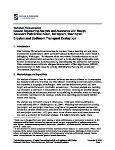
Figure 4-3. Schematic illustration of Reynolds’ experiments on the nature of fluid flow. See text for a detailed discussion.

R < 1000

1000 < R < 2000

R > 2000

Note that the shear stress acting on the boundary represents the case where y = 0 (such that D-y = D) and is termed the boundary shear stress (given the symbol τo). From Eq. 4-5:

τ

°

= ρgD sin 0

Eq. 4-6.

This is a particularly important component of fluid shear because it acts on the bottom of a flow where much sediment is transported (i.e., it is the force per unit area acting on the boundary and is the force that causes sediment in contact with the bottom to move). Given the relationship shown in Eq. 4-1 we see that the velocity gradient cannot be uniform within a fluid gravity flow but must vary from a maximum at the boundary to a minimum at the water surface. Combining Eq. 4-1 and Eq. 4-3 we derive: du

=

ρg sin 0( D − y )

dy µ By integrating Eq. 4-7 with respect to y we can solve for u (the velocity at height y above the bed):

Eq. 4-7

2

u=

0 ρg sin 0 y ( D − y )dy + c = ( yD − )+c z dudy dy = ρg sin z µ µ 2

Eq. 4-8

Given that u = 0 at y = 0 (i.e., no slip along the boundary) we find that the constant of integration (c) is equal to zero, such that: u=

ρg sin 0 µ

( yD −

y

2 )

2

Eq. 4-9

Thus, the velocity of such a flow varies as a parabolic function from 0 at the bed (y = 0) to a maximum at the surface (y = D). This velocity distribution is shown schematically in comparison to the distribution of shear stress in figure 4-2B. Classification of fluid gravity flows In his classic experiments Osborne Reynolds (circa 1883) described that fluid motion could be characterized as laminar (i.e., fluid motion follows a linear path that parallels the flow boundaries) or turbulent (i.e., fluid motion follows a chaotic path that appears to be random and varies in magnitude in 3 dimensions: it includes downstream, upward and lateral components of motion). Reynolds’ experimental set-up is schematically illustrated in figure 4-3. A tank filled with fluid was drained through a transparent tube such that the velocity of fluid flowing through the tube was dictated by the height of fluid in the tank and the tube diameter. Dye

59

was injected into the fluid at the entrance of the tube and the behaviour of the flow was visualized by watching the behaviour of the dye streak in the tube. For a given fluid and constant tube diameter Reynolds found that at low velocities the streak of dye followed a linear path through the length of the tube. At high velocities the fluid paths were very irregular and the dye was quickly distributed uniformly through the tube (i.e., no dye streak persisted through the tube). At intermediate velocities a dye streak persisted but its’ path was rather irregular and not parallel to the walls of the tube. By conducting the experiments using a variety of fluids (of different viscosity) and different tube diameters Reynolds found that he could predict whether a flow would be laminar or turbulent (the intermediate flow type is termed “transitional”) by the relationship: R=

ρUD µ

Eq. 4-10

where U is the mean flow velocity and D can be flow depth in channels that are much wider than they are deep or D can be tube or pipe diameter. Viscosity is commonly expressed as kinematic viscosity (ν, where ν = µ/ρ; SI units are m2/s) and Eq. 4-7 is commonly written: R=

UD

ν

Eq. 4-11

R is termed the flow Reynolds Number and it is dimensionless (i.e., it has no dimensions). In open channels flow is laminar when R < 500 and turbulent when R > 2000 and transitional when 500 < R < 2000 (these limits are somewhat different for flow through tubes or pipes; see Fig. 4-3). The flow Reynolds’ Number can be thought of as the ratio between inertial forces (flow inducing forces) to viscous forces (flow resisting forces). When viscous forces are large, relative to the inertial forces the structure of the flow will be dominated by viscosity (i.e., momentum is transferred by way of viscous attraction between fluid molecules) and the flow is laminar. Flow is turbulent when viscous forces are small compared to inertial forces (i.e., deep fast flows) and momentum is transferred by turbulence (see below). Fluid flows with a free surface (i.e., excluding flows in pipes) can also be classified by the another dimensionless number termed the Froude Number (F), where: F=

U gD

Eq. 4-12

F can be thought of as ratio of inertial forces acting on the fluid to gravity forces that act on the water surface. When F < 1 a flow is said to be subcritical or tranquil and when F > 1 a flow is said to be supercritical or shooting (a flow for which F = 1 is said to be critical). In practical terms F is significant in two related ways. First, the term

gD is equal to the celerity of waves on a water surface (i.e., the speed at which such waves

propagate over the water surface). As such, if F < 1 then U < gD and water surface waves will propagate upstream because their celerity is faster than the flow velocity. If F > 1 then U > gD and water surface waves will be swept downstream. A more important implication of F to our later consideration of bedforms under unidirectional flows is shown in figure 4-4. When F < 1 the water surface may be out-of-phase with a mobile sediment bed whereas when F > 1 the water surface is in-phase with the mobile sediment bed. Shear stress and velocity distribution in turbulent flows Most fluid flows that are geologically important are turbulent and their characteristics vary considerably from the laminar flows that were described earlier in this section. Among other things, because fluid motion is so irregular (and three-dimensional) turbulent flows are very difficult to treat mathematically. Thus, this section will consider turbulent flows in a much more qualitative manner. Figure 4-5 compares the velocity profiles of laminar and turbulent flows. For now, disregard the difference in turbulent flows over rough and smooth boundaries and focus on comparing the forms of the

60

F1 water su r f a c e

Water surface

Figure 4-4. Schematic illustration showing the significance of the Froude Number in terms of the phase relationship between the free water surface and a mobile sediment bed.

curves for laminar and turbulent flows. Note that the lower portions of the curves for turbulent flows are like a compressed version of the curve for laminar flow (i.e., there is an initially rapid increase in velocity away from the boundary). However, the remainder of each curve for turbulent flows shows a much lower rate of increase in velocity than does the curve for a laminar flow (i.e., in turbulent flows du/dy in the upper portion of the flow is much more uniform than is the case for laminar flows). These two features reflect the fundamental differences in the manner in which shear stress is distributed though the flows. In laminar flows the momentum of the fluid was determined by the viscous shear stress acting on that fluid within the flow. However, as figure 4-6 illustrates, in turbulent flows fluid momentum is also changed as packages of fluid move up and down throughout the flow (the characteristics of these moving packages will be described below). Low-speed fluid from near the boundary moves up into the region of high speed fluid, at some distance from the boundary, and the high speed fluid loses momentum. Conversely, high speed fluid from the region away from the boundary may move downward and increase the momentum of the fluid near the boundary. This physical movement of fluid through the flow accounts for the more uniform distribution of velocity, well above the boundary region. This transfer of momentum differs fundamentally from viscous shear stress but it has the same outcome and is often termed turbulent shear stress or reynolds stress. Viscous shear stress is also important within a turbulent flow, in fact it predominates in the region closest to the boundary where the velocity gradient is large. Thus, the total shear stress along any plane passing through a turbulent flow depends on the viscous and turbulent components of shear stress and takes a form similar to Eq. 4-1:

τ = (η + µ)

du

Eq. 4-13

dy

which can also be written: Water Surface

U

U

U

D

Laminar Flow

Turbulent Flow (smooth boundary)

Turbulent Flow (rough boundary)

Figure 4-5. Schematic illustration comparing the distribution of velocity through turbulent and laminar flows. See text for a detailed discussion.

61

turbulent shear stress

Turbulence dominated

}

D

}

du du τ =η +µ dy dy viscous shear stress

Figure 4-6. Schematic illustration of the nature of shear stress in a turbulent flow. See text for details.

Viscosity dominated

U

τ=η

du

+µ

du

Eq. 4-14 dy dy where η (the Greek letter eta) is termed the “coefficient of eddy viscosity”, a measure of the effectiveness with which momentum is transferred through the flow by eddies (packages of fluid). Figure 4-6 illustrates the above discussion and shows that the upper portions of a turbulent flow are dominated by turbulent shear stress while the region nearest the boundary is dominated by viscous shear stress. In fact, the boundary itself is so much dominated by viscous shear that the boundary shear stress for turbulent flows may be determined by the same relationship used for laminar flows. (i.e., Eq. 4-6). However, the velocity distribution within a turbulent flow is considerably different from that in a laminar flow (compare curves in Fig. 4-5) and can only be described in terms of experimentally-determined relationships: one for turbulent flow over smooth boundaries and another for rough boundaries (i.e., covered with sediment and/or bedforms composed of sediment). The formula for predicting flow velocity (u) at some distance (y) from a rough boundary (the most common type of boundary of concern in sedimentology) is given by: u

= 8. 5 +

U*

2. 3

κ

log

y yo

Eq. 4-15

where κ is termed “von Karman’s constant” and is equal to 0.4 for most fluids, yo is a measure of the height of the roughness elements on the boundary (either the grains and/or the bedforms) and U* is termed the shear velocity of the flow and it is related to the boundary shear stress by: U* =

τo

Eq. 4-16

ρ

Shear velocity has the dimensions of velocity and is a convenient way in which to express boundary shear stress. By Eq. 4-15 the velocity is zero at some point just beneath the surface of the rough boundary, in contrast to turbulent flow over smooth boundaries where velocity is zero at the boundary surface (see Fig. 45). Note that the mean velocity of a turbulent flow over a rough boundary occurs at y = 0.4D. Thus Eq. 4-15 can be used to calculate mean velocity by substituting this value. Structure of turbulent flows Turbulent flows can be subdivided into three zones on the basis of the way in which momentum is transferred (Fig. 4-7); these subdivisions are also characterized by difference in the behaviour of the flow. The viscous sublayer is the zone that extends upwards from the boundary and is dominated by viscous shear (much like a laminar flow). The thickness of the viscous sublayer (δ) is given by:

62

Figure 4-7. Subdivisions of turbulent flows based on the major mechanisms of momentum transfer. The outer layer is dominated by turbulent shear stress while the viscous sublayer is dominated by viscous shear.

outer layer

D

transition layer viscous sublayer

U

δ=

12 ν

Eq. 4-17

U*

and may range from a fraction of a millimetre to several millimetres in thickness. Many older texts refer to the viscous sublayer as the “laminar sublayer” of a turbulent flow but flow in this zone is not strictly laminar because it experiences fluctuations in velocity (in both speed and direction) due to interaction with turbulence from higher levels in the flow. The buffer layer is the zone which has characteristics that are intermediate between those of the viscous sublayer and the outer layer; it is a region of transition from turbulent shear to viscous shear. The outer layer is the zone where turbulence is dominant, i.e., momentum is transferred predominantly through turbulent shear stress. This zone extends from the free surface to the buffer layer and is characterized by eddies (packages of rotating fluid to be discussed in detail in a later section). As noted in the previous section, the velocity profile of a turbulent flow depends on the nature of the boundary (whether it is smooth or rough) and turbulent boundaries may be classified on the basis of the relationship between the thickness of the viscous sublayer and the size of the grains on the boundary. A boundary is said to be dynamically smooth when the viscous sublayer is thicker than the height of grains on the bed (i.e, the grains are entirely within the viscous sublayer) and dynamically rough when the grains are higher than the viscous sublayer (i.e., they protrude out of the viscous sublayer). This is an important concept because whether a turbulent boundary is dynamically smooth or rough will influence, among other things, the forces that act to move particles on the bed (see below). Turbulent boundaries may be classified by a form of Reynolds number termed a boundary Reynolds Number (R*, also termed a grain Reynolds number), where: R* =

U*d

Eq. 4-18

ν

where d is the average grain size of the bed material. We can easily determine R* for the condition (between dynamically smooth and rough boundaries) where a boundary is covered by spherical grains of uniform size that extend exactly to the top of the viscous sublayer (i.e., δ = d). Substituting Eq. 4-17 for d in Eq. 4-18: R* =

U*δ

ν

=

U*

ν

×

12 ν

= 12

U*

Thus, when the height of the grains on the bed is exactly equal to the thickness of the viscous sublayer, R* = 12. In actual fact, partly because natural sediments are not composed of uniform spheres, it has been found that boundaries behave as dynamically smooth when R* < 5 and as dynamically rough when R* > 70. Turbulent boundaries are said to be transitionally rough when 5 < R* < 70. Figure 4-8 schematically defines turbulent boundaries in the manner outlined above. Note that on beds of grains much larger than the thickness of the viscous sublayer the sublayer develops over the surface of the large particles.

63

δ ≈d

δ >d δ

R* < 5 Smooth

δ 70 Rough

Figure 4-8. Classification of turbulent boundaries on the basis of the relationship between the thickness of the viscous sublayer and the size of grains on the boundary.

Organized Structure of Turbulent Flows As described above, turbulent flows are characterized by a chaotic pattern of fluid flow and water particles are accelerated and decelerated in all directions due to the transfer of fluid momentum through the outer zone of the flow. However, organized structures within turbulent flows can be recognized on a variety of scales. Figure 4-9 shows a hypothetical curve depicting the variation in velocity (in the downstream direction) over time in a turbulent flow (i.e, if velocity at some depth were measured instantaneously and repeatedly over time). Note that the pattern of variation in velocity can be thought of as consisting of two components: a slowly varying component and a relatively rapidly varying component. These two components represent different patterns of organized fluid motion that act on different scales along with essentially random fluid motions. The organized patterns of motion are known to result from “structures” within a turbulent flow that behave in a quasi-regular manner. The outer layer of a turbulent flow is dominated by secondary flows and eddies of various type that interact in a complex manner. Secondary flows in the outer layer can be considered as rotating packages of fluid that spiral along an axis that is parallel to the mean flow direction; secondary flows impart a cross-channel and vertical component of fluid motion onto the mean, downstream flow. In straight channels two such spiral flows typically develop, side-by-side and counter-rotating. In sinuous or meandering channels the form of such secondary flows varies as shown in figure 4-10; one spiral at the bends of the meander (with surface flow towards the outside of the bend) and two spirals at the points of inflection between bends. In fact, channels meander because of the variation in the distribution in boundary shear stress and sediment transport that is caused by secondary flows. Boundary shear stress is greatest on the outside of the bend (enhancing erosion)

U

t Figure 4-9. Schematic illustration of the variation in downstream velocity at a point in a turbulent flow, measured over time. Solid line shows the rapidly varying component of turbulence; dashed line shows the slowly varying component of turbulence. See text for discussion.

64

A

A'

A' A B

B'

C

B

B'

C

C'

flo

w

C'

Figure 4-10. Secondary, spiral flows superimposed on the mean, downstream flow in a meandering channel. Arrows indicate the direction of the component of fluid motion due to secondary flows that are superimposed on the mean flow. See text for discussion.

and smallest on the inside of the bend, enhancing deposition. Deposition is further enhanced on the inside of the bed due to the component of flow velocity that acts from the outside towards the inside of the bend, transporting sediment in that direction. Eddies or vortices in a flow are packages of fluid that rotate about an axis that extends perpendicular to the direction of mean flow and these eddies travel in the mean direction at a speed equal to 0.8U∞, where U∞ is the free-surface velocity of the flow (i.e., the downstream velocity that the water surface is moving). They may be of smaller scale than secondary flows and may be superimposed on secondary flows. Eddies may extend through the entire thickness of the outer zone and may have smaller eddies superimposed on them. As eddies move in the mean flow direction they result in temporal and spatial variation in boundary shear stress due to the changes in the rate of shear that they induce in the viscous sublayer. Figure 4-11 shows a particular type of eddy that does not move along the flow direction but develops in the lee of a negative step on the boundary (such a step might be produced by a bedform; see below). Over such a step the flow is said to “separate”, become detached from the boundary, and becomes attached to the boundary at some point down stream. Upstream of the attachment point, below the step, the flow is directed in the upstream direction and forms a “roller vortex”, or “roller eddy”, that extends across the flow in the lee of the step. Downstream of the attachment point the flow “attaches” to the boundary and behaves essentially identical to flow before the step on the boundary. The development of such roller eddies in the lee of a step is important to the formation of many of the bedforms that will be described and discussed in the following chapters.

65

0

0

U

0

0

s v

a

Figure 4-11. Development of a roller vortex in (v) the lee of a negative step on a boundary. Curves show the velocity distribution in the flow near the boundary below. The letter “s” indicates the point where the flow separates from the boundary and the letter “a” indicates the position of the attachment point. See text for a discussion of details.

A component of the flow structure of the viscous sublayer includes a series of mean-flow-parallel, alternating (across the flow direction) rows of high-speed and low-speed fluid termed streaks (Fig. 4-12A). In the absence of sediment in transport by a current the spacing of streaks (λ) is given by:

λ U* ν

≈ 100

Eq. 4-19

This spacing increases when sediment is in transport over the bed (Weedman and Slingerland, 1985). Some of the small-scale fluctuations in velocity in a turbulent flow are due to a process termed the bursting process, or bursting cycle, that begins in the viscous sublayer due to some instability of streaks. Ideally, the bursting

A. Streaks

View looking down onto alternating high-speed and low-speed streaks in the viscous sublayer

Flow direction

B. The bursting process y

A burst

4

viscous 1 sublayer

4

3

1&2

3 2

U y

A sweep 2

2 1

3 viscous sublayer 1

3

3

4

4 U

Figure 4-12. Organized structure of the viscous sublayer. A. The distribution of alternating high- and low-speed streaks along the boundary (lengths of arrows are proportional to fluid speed). B. The bursting process or cycle. Left hand side schematically shows the behaviour of fluid in and near the viscous sublayer (numbered sequentially over time). The right hand side shows the effect of the movement of fluid on the near-boundary velocity profile (numbers correspond to events shown on the left hand side). See text for a detailed discussion.

66

Modes of particle movement A.

contact

C.

suspensive saltation

B.

saltation

D. intermittent suspension

FLOW Figure 4-13. Modes of transport of the components of bed material load. See text for detailed discussion.

cycle includes two events (Fig. 4-12B): bursts, which involve the ejection of low speed fluid away from the viscous sublayer, out into the outer layer, and sweeps, which involve the injection of high speed fluid from the outer layer, into the viscous sublayer. Note that bursts and sweeps have a significant effect on the local velocity profile and, therefore, local instantaneous boundary shear stress: high boundary shear stress under sweeps, low boundary shear stress under bursting. Most sweeps involve packages of fluid that had previously been ejected away from the boundary by bursting and many burst are initiated by disturbance of the viscous sublayer by incoming sweeps. However, while bursts and sweeps occur with similar periodicity and frequency, not every burst will result in a sweep and not every sweep will induce a burst. None-the-less, the bursting process is a particularly important process in generating turbulence and bursts may provide an effective mechanism of suspending sediment (see below). Finally, note that bursting does not require a welldeveloped viscous sublayer. Even on boundaries dominated by sediment that is much larger than the viscous sublayer the bursting process is known to occur although its origin is not well understood. SEDIMENT TRANSPORT UNDER UNIDIRECTIONAL FLOWS Unidirectional flows have the potential to transport sediment (depending on the “flow strength” and the size of sediment that is available for transport). Thus, on the basis of preserved sediments or sedimentary rocks we might be able to make some fundamental interpretations about the paleohydraulics of ancient depositional environments on the basis of an understanding of the relationship between sediment transport and flow conditions. Modes of sediment transport The sediment that is transported by unidirectional currents can be classified into two broad types: wash load and bed material load. Wash load is the part of the total sediment “load” that is transported continuously in suspension by the current; that is, fine-grained sediment (silt and clay) that is held in the main body of the current and rarely settles to the bed (it makes up generally 600 (i.e., over beds covered with very coarse particles). The decrease in β at low boundary Reynolds numbers is due to a corresponding decrease in the boundary shear stress required to move a particle because the lift force acting on the grain increases as the velocity gradient increases in the thinning viscous sub-layer (compare Eqs. 4-17 and 4-18). The value of β subsequently increases with increasing R* because the boundary shear stress required to move the grain increases as the viscous sublayer is disrupted the lift forces acting on the grain are reduced (because the strong velocity gradient in the viscous sublayer is reduced). A final, constant value of β is reached when R* exceeds approximately 600 and the lift force acting on the grains no longer varies with increasing R* and the critical boundary shear stress required to move a grain varies only with grain size. Shield’s diagram may be used to determine the boundary shear stress required to move a particle by the procedure outlined in Table 4-1, applied to the example of the maximum grain size in the bed material represented by the cumulative frequency curve shown in figure 4-14. From the results of the calculations in table 41 we may assume that the current that transported the sand represented by figure 4-14 exerted a boundary shear stress of approximately 2.13 N/m2. If the boundary shear stress were greater, larger sizes (>2.8 mm) would be preserved in the deposit (i.e., we assume that there were no limitations on the grain sizes available for transport). If the boundary shear stress were below this value, the current could not have moved the 2.8 mm sand and it would not be present in the bed material. However, this approach is limited because it does not consider all the variables that will determine the critical condition for movement. For example, the Shields’ curve does not include the effect of shape and packing (see section on grain shape). More angular particles will be more difficult to move than the spheres used in the experiments to determine the curve shown in figure 4-17. More important, however, the experimental curve is based on beds of uniform grain size. Thus, errors in estimating the critical boundary shear stress for motion over a bed will depend on the size of the particle for which to is being determined, relative to the average size of the bed material. Specifically Shields’ curve will underestimate the critical boundary shear stress to move a grain if the grain if much smaller than the average size of the grains that make up the bed on which it rests. This is because a small grain will tend to become trapped in the space between larger particles on the bed, making it more difficult to move. Conversely, Shields’ curve will overestimate the critical boundary shear stress to move a grain that is much larger than the average size of the particles that make up the bed on which it rests (Fig. 4-18). This is because a large grain will roll more easily over a bed of much finer particles than over particles of the same size. This is a major limitation on the use of Shields’ diagram (see discussion by Komar, 1987). Threshold of grain suspension The particles in transport as suspension load are supported (i.e., kept off of the bed) by the vertical component of turbulence. Middleton (1976) argued on theoretical grounds that the critical flow condition at which a particle became suspended was when the average component of turbulence that acts in the upward direction (we’ll give this the symbol “v”) is exactly equal to the settling velocity (ω) of the particle. Clearly, when the v < ω the particle will eventually settle to the bottom. Thus, Middleton’s criterion for suspension is: a grain will be suspended by a flow when upward velocity of the vertical component of turbulence exceeds its’ settling velocity. Unfortunately, the mean upward component of turbulence is difficult to measure. However, experiments have shown that the shear velocity of a flow is essentially equal to the upward component of turbulence so that Middleton’s criterion for suspension may be stated in a more practical manner as in figure 4-

72

V

Middleton's criterion for suspension: Suspension when V

ω

ω

Figure 4-19. Schematic illustration defining Middleton’s (1976) criterion for suspension of a particle. See text for a detailed discussion.

where V is the upward component of velocity due to turbulence and ω is the settling velocity of the particle.

19. Therefore, the largest grain that will be suspended by a flow (i.e., the coarsest grain size in the intermittent suspension population of a bed material) is one with a settling velocity equal to the shear velocity of the flow. So we have another means of interpreting grain size curves such as figure 4-14 in terms of the hydraulics of the currents that transported (and deposited) a sediment. Table 4-2 shows the relationship between the maximum shear velocity of a number of rivers and the settling velocity of the coarsest grain size in the intermittent suspension load of the bed material of these rivers. The theoretical relationship is respectably close. In the case of the grain size curve shown in figure 4-14 the largest grain size in the intermittent suspension load is 1.3φ (0.41 mm) and the shear velocity of the flow can be estimated by calculating the settling velocity of this grain size. We could use Stokes’ Law to calculate ω, by making all of the necessary assumptions, but we cannot overcome the error due to the fact that the grain size exceeds 0.1 mm. As an alternative, there are several experimentally-derived relationships to determine the settling velocity of particles beyond Stokes’ range, one of these is shown in figure 4-20 (for quartz-density particles in water at 20ºC). Figure 4-20 indicates that a quartz-density, spherical grain with a mean diameter of 0.41 mm has a settling velocity of 0.044 m/s. This suggests that the flow that transported the bed material had a shear velocity of 0.044 m/s. We can compare this result with that based on Shields’ diagram by determining the shear velocity produced by to = 2.13 N/m2 (see Eq. 4-16) and we find U* = 0.046 m/s, very close to that predicted by Middleton’s criterion. Figure 4-20 also shows the critical shear velocity for the initiation of movement of grains on a bed (from Shields’ diagram). Note that below the curve for the initiation of motion grains will not move. Between the two curves grains will move as part of the contact load and above the curve U* = ω grains will be in suspension. An important point that is illustrated by this figure is that very fine sand (less than 0.15 mm) tends to go into suspension essentially as soon as it begins to move. This has very important implications to a variety of sedimentary processes.

Table 4-2. Comparison of measured peak shear velocities of flows in rivers to the settling velocity of the coarsest particles in the intermittent suspension population of bed samples taken from each river. Data from Middleton, 1976. River

Middle Loup Middle Loup Niobrara Elkhorn Mississippi (at Omaha) Mississippi (at St. Louis) Rio Grande

U* (cm/s)

ω (cm/s)

7-9 ≈20 7 - 10 7-9 6.5 - 6.8 9 - 11 8 - 12

7-9 ≈20 7-9 2.5 - 5.0 2.5 - 5.0 3 - 12 ≈10

tr ac tio

grain suspension

*

0.05

U

Figure 4-20. Curves showing the critical value of U* for the initiation of motion (based on Shields’ diagram) and suspension as a function of grain size. Note that the curves apply to quartz-density grains in water at 20ºC. After Blatt, Middleton and Murray, 1980.

gr ai n

=ω

U or ω (m/s) *

0.10

n

73

e S hi

lds

'

no movement 0 0.01

0.1 1.0 Grain diameter (mm)

10.0