Power-aware Base Station Positioning for Sensor Networks Andrej Bogdanov Elitza Maneva∗ Samantha Riesenfeld† Computer Science Division University of California, Berkeley Berkeley, CA 94720

Abstract— We consider the problem of positioning data collecting base stations in a sensor network. We show that in general, the choice of positions has a marked influence on the data rate, or equivalently, the power efficiency, of the network. In our model, which is partly motivated by an experimental environmental monitoring system, the optimum data rate for a fixed layout of base stations can be found by a maximum flow algorithm. Finding the optimum layout of base stations, however, turns out to be an NP-complete problem, even in the special case of homogeneous networks. Our analysis of the optimum layout for the special case of the regular grid shows that all layouts that meet certain constraints are equally good. We also consider two classes of random graphs, chosen to model networks that might be realistically encountered, and empirically evaluate the performance of several base station positioning algorithms on instances of these classes. In comparison to manually choosing positions along the periphery of the network or randomly choosing them within the network, the algorithms tested find positions which significantly improve the data rate and power efficiency of the network. Index Terms— Sensor networks, optimization, combinatorics, graph theory

I. I NTRODUCTION Recent technological advances have allowed the development of relatively inexpensive, wireless micro sensors. Hundreds or thousands of these tiny sensors may be deployed in a network that monitors the environment and collects data about it. One of the chief constraints on the network is power—each sensor is equipped with only a small battery and must use its power efficiently to prolong the life of the network. Relative to the power required for computing, a large amount of power is required for transmitting messages to other sensors. Some types of sensor networks also contains a few base stations with a relatively unlimited power supply. ∗ †

Research supported in part by NSF ITR Grant CCR-0121555. Supported in part by an NSF Graduate Fellowship.

0-7803-8356-7/04/$20.00 (C) 2004 IEEE

The base stations collect data from the sensors and communicate with a central authority. Proposed applications for sensor networks cover a wide range of areas, including environmental observation, health care, and security. Mainwaring et al. [1] describe an experimental, real-world application in habitat monitoring. Their research exposes the requirements and constraints of certain types of sensor network systems which partially motivate our work. In habitat or environmental monitoring, it may be important not to disrupt the habitat during the period of observation, both in order to minimize environmental damage and to be able to make accurate observations. Therefore once the network is in place, it can be assumed to be static. The network should run for as long as possible on minimal power since the means to recharge sensor batteries from power sources in the environment may be limited. Scientists may also prefer not to do data aggregation in order to be able to study the logged data at a later point in time. Our general model of the sensor network is based on these requirements. The network is assumed to be static, and each sensor uses power at some rate, which can depend on the sensor, to transmit messages to other sensors within some range, which can also depend on the sensor. All the sensors recharge from a power source in the environment at the same fixed rate. Sensors produce and transmit their own messages, and they also forward other sensors’ messages. The rate at which a sensor produces messages may be specified relative to other sensors in the network. Every sensor’s messages must be routed to some base station, where the data can be processed. There are several power metrics that one can consider optimizing across the network, which may in turn lead to varying routing strategies. We consider the problem of maximizing the rate of production of data across the network while ensuring the survival of the network, that is, while respecting the power constraints of the sensors. We assume that the layout of the base stations can be chosen to optimize this rate by a centralized algorithm IEEE INFOCOM 2004

which is given complete information about the locations of sensors in the network. While this approach may be impractical for purposes of implementation, we view it as an analytical tool for understanding how the layout of the base stations can affect the data production and flow in the sensor network. In cases where the data rate is a fixed requirement of the sensor network, the inherent problem is to minimize the power required to provide a specific data rate. This is essentially equivalent to the problem we consider. For ease of analysis, we simply look at it from the inverse perspective: given a fixed recharging rate, how can we maximize the data rate? The experimental instance described in [1] uses one base station, located at a nearby ranger station, that collects data from the sensor network and relays it. If it is possible to provide power to a couple of more strategically placed base stations, our work suggests that the network in [1] might be able to generate a much higher data rate (or equivalently, last much longer). Our results show that in general the choice of layout for base stations in a sensor network has a marked influence on the data rate, or equivalently the power efficiency, of the network. Given the means to provide power to base stations at sensor positions, in many networks one can achieve rates much better than those achieved by manually choosing positions along the periphery of the network or randomly choosing them within the network. Our empirical evidence indicates that choosing positions with, for example, a local search algorithm, can significantly improve the data rate and power efficiency of the network. For each layout of a fixed number of base stations in the network, there is a maximum rate of data production that does not violate the power constraints of the sensors. That is, for each layout of base stations, there is a maximum feasible rate. To simplify the analysis of the problem, we assume that the possible locations of the base stations are exactly the locations of the sensors. The objective is to find a layout for the base stations which maximizes the feasible rate. We call this problem the base station positioning, or BSP, problem. In order to compare layouts of base stations, it is necessary to know the maximum feasible rates permitted by each layout. Therefore we first focus on the problem of computing the maximum feasible rate for a fixed layout of base stations. We show that this problem reduces to a max-flow min-cut problem on a flow network. Our analysis gives a natural upper bound on the rate and then shows that this upper bound is actually feasible. In fact, in our experiments, we use implementations of a max-flow algorithm to compute it efficiently. 0-7803-8356-7/04/$20.00 (C) 2004 IEEE

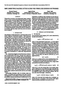
Although this problem turns out to have an efficiently computable solution, the larger problem of choosing the optimum layout of base stations turns out to be NP-complete. In fact, the BSP problem is NP-complete even when the sensor networks are restricted to be homogeneous, that is, restricted so that every sensor has the same range of transmission, power usage, and rate of message production. We give a reduction from the NPcomplete dominating set problem on unit disk graphs. Homogeneous sensor networks can be represented by geometric (or unit disk) graphs. We consider the BSP problem on several types of geometric graphs. In the case of the regular grid, we are able to give an analysis of the optimum layout of base stations. In fact, we show that all layouts that meets certain conditions are equally good. The other two types of geometric graphs that we consider are randomized and designed to approximate irregular sensor networks that might occur in the real world. We turn to several heuristic algorithms for solving the BSP problem on these types of geometric graphs. None of the efficient algorithms tested offers a guarantee on its performance, but in our experiments they perform well. The exhaustive search algorithm is guaranteed to give an optimum solution, and therefore is useful for comparison, but is impractical on examples with more than a couple of base stations. The local search hill-climbing algorithm is more practical and performs very well—it found optimum solutions for every case on which we also ran the exhaustive search. The greedy algorithm is more efficient, but does not generally perform as well. In Figure 1 we give an example of a solution found by one of the algorithms tested. The graph is the largest connected component of a geometric graph on uniformly distributed vertices. The large white vertices are the base stations, as positioned by the algorithm. The gray vertices form a vertex separator for the base stations and constitute the “bottleneck” for the rate of data production and flow. The rest of the paper is organized as follows: In the next section, we briefly summarize previous related research and compare it with the work in this paper. In Section III, we show how to compute the maximum possible rate for a fixed layout of base stations by reduction to maximum flow. In that section we also give the NP-completeness proof for the base station positioning (BSP) problem. We describe several restricted classes of sensor networks, which can be represented by geometric graphs, and justify our interest in these classes in Section IV. A detailed analysis of the optimum layout in the special case of the regular grid follows in Section V. We discuss our selection of heuristic BSP algorithms IEEE INFOCOM 2004

Fig. 1. A uniform random sensor network on 300 nodes with four base stations. The large white vertices are the base stations. The smaller gray vertices constitute the “bottleneck”.

along with their relative merits and disadvantages in Section VI. In Section VII, we chart and evaluate the empirical performance of these algorithms. Finally, our concluding remarks and possible future directions are offered in Section VIII. II. R ELATED W ORK One aspect of the base station positioning problem is computing the maximum rate for a fixed layout of the base stations. Chang and Tassiulas [2], [3] consider a more general version of this problem. They formulate a routing multi-commodity flow problem with node capacities as a linear program, where the objective is to maximize the lifetime of the system. In [2], the authors note that if the transmitted power level and node capacity at each node are fixed, then the problem is equivalent to a maximum flow problem with arc capacities, although they do not explicitly give the analysis. We independently came to the same conclusion and give the maximum flow formulation in this paper. An advantage of explicitly analyzing this simpler version of the problem, which is all that is needed for our model, is the simple description of the optimum solution afforded by the max-flow min-cut theorem. Moreover, existing fast implementations of maximum flow algorithms (e.g., [4]) can be used to implement the base station positioning algorithms. Power-efficient distribution and collection of data in sensor networks has also been studied for other net0-7803-8356-7/04/$20.00 (C) 2004 IEEE

work models and optimization metrics. Florens and McEliece [5], [6] consider the effect of interference on inter-sensor communication and show how to obtain schedules with near-optimum makespan for data collection with a single base station. Their model, however, does not explicitly address power consumption. Other approaches include minimizing packet length through data compression [7], selectively shutting off sections of the network while maintaining connectivity [8], exploiting the clustered structure of networks [9], [10], and varying the routing strategy with time [11]. Another variation is online routing, where the rate of transmission and the message sequence may not be known in advance [12], [13]. The base station positioning problem has also been studied in the context of cellular (UMTS) networks. Galota et al. [14] exhibit a polynomial time approximation scheme that maximizes the overall utility of base station positioning for a fairly comprehensive model, which includes parameters such as construction costs, operating costs, customer satisfaction and noise interference. The proposed algorithm is significant from a theoretical standpoint, but would be difficult to implement. We also note that cellular network models are generally different from our network sensor model, since in such networks, nodes are not capable of forwarding other nodes’ messages. Another type of network closely related to our model is the packet radio network. In these networks, the power used by a vertex to transmit a message at distance d is typically modeled as cd−α , where c and α are parameters of the model. One problem is to assign transmission ranges to nodes so as to minimize total power, under the constraint that the network is strongly connected. Kirousis et al. [15] show algorithms and lower bounds for this problem when the nodes lie either on a line or in three-dimensional space. Clementi et al. [16] derive an approximation algorithm for the planar version, though it is apparently not known if an efficiently computable exact solution is possible for this case. We are not aware, however, of any work that considers the effect of base stations on power consumption in these networks. III. C OMPUTING

THE RATE OF TRANSMISSION

In our model, each sensor has the following characteristics: 1) Position (xv , yv ) in the unit square [0, 1] × [0, 1]. 2) Reachability radius rv ≥ 0: Sensor v can send messages to sensor w if the Euclidean distance between (xv , yv ) and (xw , yw ) is at most rv .

IEEE INFOCOM 2004

3) Relative importance iv > 0: The rate at which sensor v produces messages should be proportional to iv . 4) Capacity cv > 0: This is the number of messages that the sensor can send in unit time without violating its power constraints. The connectivity graph G of the sensor network is the digraph on vertex set V = {1, . . . , n}, where (v, w) is an edge if w is within the reachability radius of v . For a fixed collection of base stations B ⊆ V , a flow fv from vertex v is an assignment of nonnegative weights wp to all directed paths p that start at v and end at some base station b ∈ B . Given a collection of flows F and an vertex v of G, we use f (v) to denote the combined weight of the flows passing through v , i.e.,

f (v) = wp . f ∈F p∈f :v∈p

Similarly, for an edge e, let f (e) denote the combined weight of the flows going through e, in the direction of e. A routing strategy of rate ρ is a collection of flows f1 , . . . , fn that satisfy the following constraints: 1) Importance constraint: For each vertex v ∈ B ,  w = ρiv . p p∈fv 2) Capacity constraint: For each vertex v ∈ B , the total flow into v does not exceed the capacity of v , i.e., f (v) ≤ cv . We are interested in the maximum rate ρ∗ for which there exist flows satisfying these constraints. To obtain a handle on this value, it is useful to introduce another notion. A separator is an arbitrary subset of V − B ; we say a vertex v is separated by S if every path from v to B intersects S . Let L(S) denote the set of vertices separated by S . In particular, S ⊆ L(S). For any separator S , we observe that the flow originating from L(S) cannot exceed the total capacity of S , from where we obtain the following upper bound on any achievable rate:  cv ρ ≤  v∈S . v∈L(S) iv We show that this upper bound is achievable: Theorem 1: There existsa separator S such that the c maximum rate ρ∗ equals  v∈S viv . v∈L(S)

Proof: We will derive this statement by reduction from the max-flow min-cut theorem for directed flow networks with arc capacities. We construct an instance G (ρ) = (V  , E  ) of a digraph with arc capacities as follows:

0-7803-8356-7/04/$20.00 (C) 2004 IEEE

1) The vertex set V  consists of: a source node s; a sink node t; for each vertex (sensor) v ∈ V , a “receiver node” sv and a “sender node” tv . 2) (Type 1 arcs) For each vertex v ∈ V , G contains an arc s → sv of capacity ρiv . 3) (Type 2 arcs) For each base station b, G contains an arc sb → tb of infinite capacity. 4) (Type 3 arcs) For each vertex v ∈ V , G contains an arc sv → tv of capacity cv . 5) (Type 4 arcs) For each edge v → w of G, G contains an arc tv → sw of infinite capacity. We note that all finite (s, t) cuts in G have a special form: Any such cut is completely determined by a separator S , and consists of two types of arcs: (1) Type 1 arcs from s to vertices in V − L(S) and (2) Type 3 arcs determined by vertices in S . We now consider what happens to the minimum (s, t) cut in G (ρ) as we vary ρ continuously. When ρ = 0, the cut (s, V  − s) is a minimum (s, t) cut of G with value 0. By continuity, there must exist a largest value ρ∗ ∈ [0, ∞) for which (s, V  − s) is a minimum (s, t) cut. It follows that, at ρ = ρ∗ , a new minimum (s, t) cut (S  , V  − S  ) appears in the network. Let S be the separator in G that determines this cut. ∗  At ρ ∗ = ρ , the value of the cut (s, V − s) is the value of the cut v∈V ρ iv . On the   other hand,    ∗ (S , V − S ) is v∈L(S) ρ iv + v∈S cv . Since both of these cuts are minimum, they must be equal, from where:  cv ∗ ρ =  v∈S . v∈L(S) iv

It remains to show that ρ∗ can be interpreted as the rate of some routing strategy in G. Let fst denote a maximum (s, t) flow in G (ρ∗ ). Since (s, V  − s) is a minimum (s, t) cut in G (ρ∗ ), fst must saturate all of the arcs of type 1. For each v ∈ V , we now define fv as the portion of the flow fst that uses edge (s, sv ) ∈ E  . We obtain the flow fv in G by contracting type 3 arcs and ignoring type 1 and type 2 edges in fv . It is not difficult to check that the flows {fv } determine a routing strategy of rate ρ∗ for G. The proof of Theorem 1 suggests a natural algorithm for finding the flows (message paths) that achieve optimal rate for a fixed B : Reduce the instance to a network flow problem, as in the proof, and apply a maximum flow finding algorithm to the reduced instance. The maximum flow problem has been studied extensively, and admits a host of algorithms that do not only guarantee good worst-case behavior but also perform well in practice. For our empirical evaluation we used an implementation of the Goldberg-Tarjan algorithm [17] by Cherkassky and Goldberg [4]. IEEE INFOCOM 2004

In what follows, we will assume that cv = 1, iv = 1, and rv = r for all v . In the sensor network world, this essentially means that all sensors are alike. The condition cv = 1 means that all sensors renew their power at the same rate; iv = 1 means that they all have the same importance; rv = r means that their transmission radius (which is some function of their transmission power) is the same. In particular, in this case the connectivity graph becomes undirected. As we vary the positions of the base stations, the problem of finding a base station layout that achieves the best possible flow becomes hard, even in the restricted case cv = iv = 1, rv = r. More formally, we consider the following decision problem, which we call BSP (for base station positioning): I NPUT: A collection of vertex position pairs (x1 , y1 ), . . . , (xn , yn ) ∈ [0, 1] × [0, 1], a number of base stations 0 ≤ b ≤ n, a rate ρ ∈ [0, 1] P ROBLEM : Decide whether there exists a layout of b base stations on top of the vertices that admits a routing strategy of rate at least ρ Claim 1: The BSP problem is NP-complete. Proof: BSP is easily seen to be in NP, as the optimum base station positioning can be certified to achieve rate ≥ ρ by performing a maximum flow computation, using the reduction from the proof of Theorem 1. To show NP-hardness, we exhibit a reduction from dominating set on unit disk graphs. The NP-hardness of this problem is shown in [18]. We observe that a fixed layout of base stations B admits a routing strategy of rate 1 if and only if it is a dominating set for the connectivity graph: If B is a dominating set, then each vertex can send a flow of value 1 directly to an arbitrary neighbor in B . Conversely, suppose that B admits a flow of rate 1. Now consider the separator S consisting of all neighbors of B (except for the vertices in B itself). By our upper bound on the rate, we must have 1 ≤ |S|/|L(S)|, from where |V − B| = |L(S)| ≤ |S| = |neighbors of B|.

Therefore, every vertex in V − B is a neighbor of B , so B is a dominating set. It follows that BSP with ρ = 1 is equivalent to dominating set on unit disk graphs. IV. C LASSES

OF SENSOR NETWORKS

Given the apparent difficulty of solving the BSP problem exactly on general sensor networks, we restrict our attention to several classes of homogeneous networks. A homogeneous network is one in which all sensors are essentially the same, that is, cv = iv = 1 and rv = r

0-7803-8356-7/04/$20.00 (C) 2004 IEEE

for all sensors v . Such networks can be represented by geometric graphs. A graph G = (V, E) is called geometric with connectivity r if there is an edge e = (u, v) ∈ E if and only if dist(u, v) ≤ r. That is, there is an edge between two vertices if and only if the corresponding sensors are within each other’s transmission radius. We consider three classes of geometric graphs: the regular grid, the uniform random graph, and the preferential attachment graph. All graphs are contained in the [0, 1]×[0, 1] square of the Euclidean plane, which we call the unit square. In the regular grid, the vertices are spaced evenly at regular intervals in the unit square. The interval distances in the x and y directions are equal and depend only on the number of vertices. The grid models a type of sensor network that measures some characteristic of the environment at regular intervals of distance. Such a network might be used, for example, in agriculture. The uniform random graph is constructed by dropping points uniformly at random in the unit square. This graph is designed to imitate the types of networks that might be formed by a plane dropping sensors at random over a small area. These types of sensor networks may be constructed in environments which are not easily accessible or in which so many sensors are being deployed that it is not feasible to position them individually. The last class of geometric graphs we consider is the preferential attachment graph. The construction of the preferential attachment graph depends on a parameter p, where 0 ≤ p ≤ 1. The vertices are positioned sequentially as follows: with probability p, a vertex v is dropped uniformly at random in the unit square; with probability 1 − p, v is positioned uniformly at random in the disc of radius r about a vertex w, which is chosen uniformly at random from those vertices already positioned. (Note that if the disc of radius r about w is not contained within the unit square, v is positioned uniformly at random in the intersection of this disc with the unit square.) This class of graphs tends to have higher clustering than the uniform random graph, depending on the value of p, and models types of interaction that occur in more complex networks. It is inspired by proportional attachment models of the World Wide Web [19], [20], [21]. In the case of the regular grid, we are able to give a theoretical analysis of the optimum layout of base stations, which is confirmed by the results of the experiments. Instances of the other two classes of graphs are used to further test and evaluate the base station positioning algorithms. The algorithms we use are designed to work on connected graphs. Therefore, we filter instances of uniform random graphs and preferential attachment IEEE INFOCOM 2004

graphs so that only the largest connected component remains. V. A NALYSIS

FOR THE GRID

For the grid, it is convenient to rescale the bounding √ box by n − 1 so that the geometric distance between consecutive points becomes 1. We call a set W ⊆ V l-centered if the distance between any v ∈ W and the border of the grid is at least l. We call W l-dispersed if the distance between any pair of distinct v, w ∈ W is at least l. √ Theorem 2: Assume b = |B| = o( n/r). Let d = √ r( b + k), where k is a constant that does not depend on n, r, or b. All r-centered, d-dispersed base station layouts achieve the maximum rate. Moreover, the value of this rate is (πr2 − O(r))b/(n − b). For the analysis, it will be natural to approximate separators by continuous two-dimensional subsets of the plane, which we will call “planar separators”, as follows: We imagine replacing each vertex v in the separator by a unit square centered at (xv , yv ) with edges parallel to the coordinate axes. The number of vertices in the graph-theoretic separator then equals the area of its corresponding planar separator. More generally, a planar separator can be an arbitrary √ √ (measurable) set of points in the n × n grid. We say that planar separator S separates points p and q in the plane if every path from p to q contains a section of length at least r within S . Intuitively, this means that a “useful” planar separator must have “thickness” at least r. For a single vertex v ∈ V , we say that planar separator S separates v if S separates v from all the base stations. In general, the surface area of a planar separator may be smaller than the number of vertices in it. However, in what follows, the difference between the surface area and the number of vertices in a planar separator will be small enough to have a negligible effect on our computations, and ultimately no effect on the analysis. Given a convex polygon P in the plane, the l-envelope of P (Figure 2(a)), which we denote by envl (P ). is the curve obtained by applying the following transformation to P : 1) Translate every line segment e of P by a vector of length l perpendicular to e, pointing outward from P; 2) Connect the translated segments by circular arcs of radius l centered at the vertices of P . This definition can be extended, by continuity, to arbitrary closed convex curves C in the plane since any such curve C can be approximated arbitrarily closely

0-7803-8356-7/04/$20.00 (C) 2004 IEEE

envl (P )

beltl (P )

ext(S)

P

int(S) ∂int (S) S

∂ext (S)

Fig. 2. (a) The envelope and belt of a polygon; (b) The interior, exterior, and boundary of a separator.

by a polygon. We define the l-belt of C as the section of the plane between C and the l-envelope of C : beltl (C) = ∪l ∈[0,l] envl (C). It is not difficult to see that length(envl (C)) = length(C)+2πl and area(beltl (C)) = l · length(C) + πl2 . Let S be a separator that is contractible to a simple closed curve. By the Jordan curve theorem [22], S partitions the plane into three regions (Figure 2(b)): A bounded interior int(S), an unbounded exterior ext(S), and S itself. We write ∂int (S) for the boundary between S and int(S), and ∂ext (S) for the boundary between S and ext(S). Note that the r-belt of any closed convex curve separates int(S) from ext(S). Lemma 1: Among all separators in S of area at most A that contract to a simple closed curve and separate int(S) from ext(S), the r-belt of the circle of radius A r 2πr − 2 maximizes the area of int(S). Proof: Let S0 denote the separator that maximizes area(int(S)). It is not difficult to see that S0 must be the r-belt of some closed convex curve: Convexifying S0 may only increase area(int(S)), and among all convex curves S with fixed ∂int (S), the r-belt minimizes area(S). Let P = length(∂int (S0 )). Then area(S0 ) = rP +πr2 , so the problem of maximizing area(int(S)) for fixed area(S) is equivalent to the problem of maximizing area(int(S)) given P = length(∂int (S)). The celebrated isoperimetric theorem says that the optimum choice for S is the circle of radius P/2π . Proof of Theorem 2: Let S(v) denote the ball of radius r centered at v ∈ V , excluding v itself, and S0 = ∪v∈B S(v). We will show that if B is r-centered and ddispersed, then the ratio |S|/|L(S)| is minimized when S = S0 . By Theorem 1, it follows that the maximum achievable rate is b|S(b0 )| |S0 | = ρ∗ = |L(S0 )| n−b b(πr2 − O(r)) b(area(S(b0 )) − O(r)) = , = n−b n−b where b0 is an arbitrary base station.

IEEE INFOCOM 2004

We now relax our definition of “separator” to allow for arbitrary planar separator, and show that the planar version of S0 minimizes the ratio area(S)/area(L(S)). To reach a contradiction, suppose there exists a planar separator S such that area(S)/area(L(S)) < area(S0 )/area(L(S0 )). Without loss of generality, we may assume that each connected component of S separates two regions of the plane and contracts to either (1) a simple closed curve or (2) a simple open curve whose endpoints lie on the boundary of the grid. Moreover, the interiors of the type (1) curves are pairwise disjoint. This can be seen by case analysis over the possibilities for the topology of S , using the dispersion property of B . Now consider an arbitrary component S  of S of type (1). The argument for type (2) components is similar. Let B  = B ∩ int(S  ), and b = |B  |. We will show that the optimality of S implies b = 1, so that S  = S(b0 ), where b0 is the unique element of B  . First, suppose that b = 0, so that int(S  ) contains no base stations. We show that getting rid of this part of the separator only improves, i.e. decreases, the ratio area(S)/area(L(S)). In this case int(S  ) ∪ S  ⊆ L(S). Since S is optimal, area(S − S  ) area(S) ≤ area(L(S)) area(L(S) − (int(S  ) ∪ S  )) area(S) − area(S  ) . = area(L(S)) − area(int(S  ) ∪ S  ) This condition holds if and only if    area(S)/area(L(S)) ≥ area(S )/area(int(S ) ∪ S ), so that πr2 b area(S0 ) = n−b area(L(S0 )) area(S) area(S  ) ≥ ≥ . area(L(S)) area(int(S  ) ∪ S  )

By Lemma 1, for fixed area(S  ), the right-hand side is minimized when S  is the r-belt of a circle. Let R denote √ the radius of this circle, so that R + r ≤ n/2. Then 2πRr + πr2 r πr2 b r ≥ ≥√ ≥ , 2 n−b π(R + r) R+r n/2 √ from where b ≥ n/(1 + πr n/2), contradicting the √ assumption b = o( n/r). Now suppose that b ≥ 2. In this case, int(S  ) ∩ L(S) = ∅. We will show that area(S  ) > πr2 b = area(∪v∈B  S(v)), contradicting the optimality of S . Let C denote the convex hull of B  , and S  be the r-belt of C (Figure 3(a)). The set S  is the minimum area separator such that B  ⊆ int(S  ), and in particular

0-7803-8356-7/04/$20.00 (C) 2004 IEEE

S 

S 

C S



Fig. 3. The sets C  , S  and S  . The black dots indicate the base stations within int(S  ), and the shaded areas around them are neighborhoods of radius l/2.

area(S  ) ≤ area(S  ). Finally, let C  denote the d/2envelope of C , so that length(C  ) = length(C) + πd = area(S  )/r + π(d − r) ≤ area(S  )/r + π(d − r).

By the isoperimetric theorem, length(C  )2 /4π , so that

area(int(C  ))

≤

4π area(int(C  )) ≤ (area(S  )/r + π(d − r))2 .

Now consider the collection of disks centered at the points of B  of radius d/2 each (Figure 3(b)). Since B is d-dispersed, these disks are pairwise disjoint. Moreover, their union is completely covered by int(C  ), so that area(int(C  )) ≥ π(d/2)2 b , and √ πd b ≤ area(S  )/r + π(d − r). By the optimality of S  , area(S  ) ≤ πr2 b , so that √ πd b ≤ πrb + π(d − r) √ √ from where d ≤ r( b + 1) ≤√ r( b + 1), which contradicts the assumption d = r( b + k). An interesting case not covered by the analysis occurs √ when b = Ω( n/r). One suspects that, even past the √ point b = n/r, a flow of (πr2 −O(r))b/(n−b) remains feasible, but is not necessarily achieved by an arbitrary d-dispersed base station layout. VI. P OSITIONING

THE BASE STATIONS

Our analysis provides a way to evaluate different strategies for laying out base stations on an arbitrary network. In many current applications the positions of the base stations are usually limited by the positions of power sources. Often these sources are on the periphery of the network. However, in some situations it may be worth adding a power source at a different location to improve the power requirements at the sensors. Ideally, one would like to know what is the best layout of b base stations in the network. This is the BSP problem, defined in Section III, where we show IEEE INFOCOM 2004

that for a variable number of base stations, it is NPhard. The existence of a polynomial time approximation scheme for this problem is still an open question. To the best of our knowledge, it has not been studied before, and approximation algorithms with any guarantee on the approximation factor are not known. We designed and tested several heuristic algorithms for finding good layouts for the base stations. All of these algorithms use as a black box the procedure for computing the rate achieved by a particular configuration of base stations. We compare their performance to choosing the positions at random, as well as to a manual choice of base station positions on the periphery. A. Greedy Algorithm The greedy algorithm picks the position of base stations one-by-one in a greedy manner. That is, it consecutively chooses the position of each base station to improve the rate as much as possible, while keeping the previous base stations fixed. The greedy algorithm is deterministic and runs the black box procedure O(bn) times. When there is no choice of position for the next base station that improves the rate, we restrict the algorithm to choosing a position in L(S), the set of sensors on the side of the vertex separator opposite the base stations already positioned. This restriction becomes important in situations where L(S) has two or more disconnected components, since without it, the greedy algorithm might keep placing base stations on one side of the vertex separator, missing any future chance to improve the rate. Even with the restriction, this situation is a weak point of the greedy algorithm. A better algorithm needs the freedom to change the previously chosen positions of the base stations. B. Local Search Algorithm The local search algorithm starts with a random configuration of the base stations. Then it checks if the rate can be improved by moving any of the base stations to a neighboring node. If possible, it makes such a move and repeats. When no improvement is possible, the algorithm has reached a local maximum, at which point it records the current rate. The algorithm restarts from a different random configuration a linear (in the number of nodes) number of times, and it outputs the highest local maximum it encounters. The number of steps that the local search can take is bounded by the number of different discrete values for the rate that we allow, which is typically not very large (for example it’s 1000 when we consider the rate up to 3 significant digits).

0-7803-8356-7/04/$20.00 (C) 2004 IEEE

It is conceivable that one may be able to improve the local search algorithm by allowing it to make moves that decrease the rate. This is commonly known as a Metropolis algorithm. The difficulty in implementing this algorithm is choosing good transition probabilities. The transition probabilities should simultaneously give enough weight to high-rate layouts and guarantee fast mixing time for the random walk performed by the algorithm in the space of possible layouts. VII. E MPIRICAL

RESULTS AND OBSERVATIONS

We tested our algorithms on the three models of graphs described in Section IV: The regular grid, a uniform random graph, and a random graph with preferential attachment. We set iv = 1, for all v , so that all sensors need to generate data at the same rate: once per time step. We compare the amount of power that sensors require per time step for the best layouts of base stations found by each algorithm. Minimizing the power usage for a fixed data rate is the same as maximizing the data rate for fixed power, so we could equivalently compare the maximum data rates achieved for different layouts. We ran each algorithm on a 10 × 10 grid with radius 2.2, a uniform random graph with 300 vertices and radius 0.1, and on a preferential attachment graph with 300 vertices, radius 0.1, and p = 0.4. The best lower bound that we have on the optimum power usage is 1, since every sensor has to send out at least its own messages. One can find the optimum layout in time O(nb ) by exhaustive search, which is feasible for small values of b. In our examples on 300 nodes we used exhaustive search for up to three base stations. For comparison, we took 100 random samples of layouts and computed their power usage. It is no surprise that the choice of layout turns out to influence the power requirements very significantly. One possible strategy for positioning base stations is to choose the best out of a linear number of random samples. However, our simulation shows that in many cases employing the local search algorithm may result in a layout that has about half the power usage. We also experimented with choosing layouts of base stations on the periphery of the graphs, in an effort to mimic current practice. Our data seems to suggest that for a uniform random graph, this method generally does not lead to a good layout and performs worse than an average random layout and much worse than layouts found by our algorithms. Interestingly, for the preferential attachment model, peripheral layouts appear to perform almost as well a random layout, and we attribute that to the fact that human intuition works well on the preferential attachment graphs, because there are IEEE INFOCOM 2004

Fig. 4. Peripheral layout with five base stations on a preferential attachment graph.

Fig. 5. The optimum solution with 4 bases stations on 10 × 10 grid. 7 random samples greedy algorithm local search

0-7803-8356-7/04/$20.00 (C) 2004 IEEE

6

5 power useage rate

generally very clearly expressed clusters, many of which are close to the periphery. Figure 4 shows the peripheral layout with five base stations in the preferential attachment model. Our local search algorithm appears to find solutions that are close to the optimum. We are able to check this empirically for up to three base stations. In these cases local search found the optimum. We did not observe any significant improvement in the rate output by our implementation of the Metropolis algorithm as compared to the local search algorithm. The greedy algorithm also achieved lower power requirements than the random samples in general, but still did not do as well as the local search algorithm. On the other hand, it still has the advantage over the local search that it is deterministic and of small complexity. The results on a regular grid, shown on Figure 6, verified our analysis from Section V. Initially the optimum power usage is inversely proportional to the number of base stations. When the network becomes saturated with base stations, the added base stations yield smaller power savings. In our 10 × 10 example, there exists a solution with 8 base stations in which all sensors neighbor a base station. The solutions found by local search for the cases of one to four base stations are provably optimal. For example Figure 5 shows a way to pack 4 base stations in the square, which is an optimum solution found by local search. The greedy algorithm does not perform as well on the grid, because it does not manage to efficiently

4

3

2

1 1

Fig. 6.

2

3

4

5 6 number of base stations

7

8

9

10

Power usage for the grid.

pack the disks of base stations’ neighbors into the square. The measurements for the uniform random graph and the preferential attachment graph are shown in Figure 7 and Figure 8, respectively. VIII. C ONCLUSION We consider the problem of optimizing the positions of base stations in a data collecting sensor network to minimize the power consumed by the sensors. We show by simulation that significant improvements can be achieved by employing an algorithm such as local search to find a layout for the base stations. An interesting extension of our work would be the design of a routing protocol that uses the flow assignments found by our maximum flow procedure. One of the issues that such a protocol might need to address is the effect of interference between message transmissions. IEEE INFOCOM 2004

100

80 random samples peripheral placement greedy algorithm local search

90

random samples peripheral placement greedy algorithm local search

70

80 60

power useage rate

power useage rate

70 60 50 40

50

40

30

30 20 20 10

10

1

2

3 number of base stations

4

5

1

20 random samples peripheral placement greedy algorithm local search

18

3 number of base stations

4

5

random samples peripheral placement greedy algorithm local search

18

16

16

14

14 power useage rate

power useage rate

2

20

12 10 8

12 10 8

6

6

4

4

2

2 6

8

10

12

14

16

18

20

number of base stations

6

8

10

12

14

16

18

20

number of base stations

Fig. 7. Power usage for the uniform random graph with (a) 1-5 base stations (b) 6-20 base stations.

Fig. 8. Power usage for the preferential attachment graph with (a) 1-5 base stations (b) 6-20 base stations.

Another future direction we are considering is the design of a polynomial time approximation algorithm with a guarantee on the quality of the solutions it finds. Such an algorithm might not be practical to implement but would be interesting theoretically and potentially useful experimentally for evaluating other algorithms. A somewhat unnatural restriction of our model is the requirement that base stations be positioned at sensor locations. This restriction is useful because it ensures that the network connectivity is independent of the positions of the base stations. It would be interesting to study how relaxing this restriction affects the value of the flow. One possible approach might be to consider a discretized version of the problem, as one expects that small changes in the base station positions should not change the network connectivity. It is not clear, however, how to ensure that such an approach is computationally feasible. More generally, it would be interesting to consider a variant of our model in which a fraction of sensors are allowed to run out of power, as long as the network remains connected. We note that our analysis does not immediately extend to this version of the problem.

ACKNOWLEDGMENTS

0-7803-8356-7/04/$20.00 (C) 2004 IEEE

We thank David Culler, Eric Brewer, and Stephen Sorkin for helpful discussions, and an anonymous INFOCOM referee for useful comments. R EFERENCES [1] Alan Mainwaring, Joseph Polastre, Robert Szewczyk, David Culler, and John Anderson, “Wireless sensor networks for habitat monitoring,” in The First ACM International Workshop on Wireless Sensor Networks and Applications (WSNA), 2002. [2] Jae-Hwan Chang and Leandros Tassiulas, “Energy conserving routing in wireless ad-hoc networks,” in Proceedings of IEEE Infocom2000, 2000, pp. 22–31. [3] Jae-Hwan Chang and Leandros Tassiulas, “Fast approximate algorithms for maximum lifetime routing in wireless ad-hoc networks,” in NETWORKING 2000, Broadband Communications, High Performance Networking, and Performance of Communication Networks. 2000, vol. 1815 of Lecture Notes in Computer Science, pp. 702–713, Springer. [4] Boris Cherkassky and Andrew Goldberg, “On implementing push-relabel method for the maximum flow problem,” in Proceedings of the 4th International Programming and Combinatorial Optimization Conference, 1995, pp. 157–171. [5] C´edric Florens and Robert McEliece, “Scheduling algorithms for wireless ad-hoc sensor networks,” in Proceedings of the IEEE Global Telecommunications Conference 2002, 2002.

IEEE INFOCOM 2004

[6] C´edric Florens and Robert McEliece, “Packets distribution algorithms for sensor networks,” in Proceedings of IEEE Infocom2003, 2003. [7] Jim Chou, Dragan Petrovi´c, and Kannan Ramchandran, “A distributed and adaptive signal processing approach to reducing energy consumption in sensor networks,” in Proceedings of IEEE Infocom2003, 2003. [8] Sanjay Shakkottai, R. Srikant, and Ness B. Shroff, “Unreliable sensor grids: Coverage, connectivity and diameter,” in Proceedings of IEEE Infocom2003, 2003. [9] Vikas Kawadia and P. R. Kumar, “Power control and clustering in ad hoc networks,” in Proceedings of IEEE Infocom2003, 2003. [10] Rabiner Heinzelman, Anantha Chandrakasan, and Hari Balakrishnan, “Energy-efficient communication protocol for wireless microsensor networks,” in Proceedings of the Hawaii International Conference on System Sciences, 2000. [11] John Byers and Gabriel Nasser, “Utility-based decision-making in wireless sensor networks,” in Proceedings of IEEE MobiHOC 2000, 2000, pp. 143–144. [12] Koushik Kar, Murali Kodialam, T. V. Lakshman, and Leandros Tassiulas, “Routing for network capacity maximization in energy-constrained ad-hoc networks,” in Proceedings of IEEE Infocom2003, 2003. [13] Qun Li, Javed A. Aslam, and Daniela Rus, “Online power-aware routing in wireless ad-hoc networks,” in Mobile Computing and Networking, 2001, pp. 97–107. [14] Matthias Galota, Christian Glaßer, Steffen Reith, and Herbert Vollmer, “A polynomial-time approximation scheme for base station positioning in UMTS networks,” in Proceedings of the 5th Conference on Discrete Algorithms and Methods for Mobile Computing and Communications, 2001, pp. 52–59. [15] Lefteris Kirousis, Evangelos Kranakis, Danny Krizanc, and Andrzej Pelc, “Power consumption in packet radio networks,” Theoretical Computer Science, , no. 243, pp. 289–305, 2000. [16] Andrea E. F. Clementi, Paolo Penna, and Riccardo Silvestri, “On the power assignment problem in radio networks,” Electronic Colloquium on Computational Complexity (ECCC), vol. 1, no. 054, 2000. [17] Andrew Goldberg and Robert Tarjan, “A new approach to the maximum-flow problem,” Journal of the ACM (JACM), vol. 35, no. 4, pp. 921–940, 1988. [18] B. N. Clark, C. J. Colbourn, and D. S. Johnson, “Unit disk graphs,” Discrete Mathematics, vol. 86, pp. 165–177, 1990. [19] R´eka Albert and Albert-L´aszl´o Barab´asi, “Statistical mechanics of complex networks,” Review of Modern Physics, vol. 74, pp. 47–97, 2002. [20] David Aldous, “A tractable complex network model based on the stochastic mean-field model of distance,” 2003, math.PR/0304701. [21] Alex Fabrikant, Elias Koutsoupias, and Christos Papadimitriou, “Heuristically optimized trade-offs: A new paradigm for power laws in the internet,” in Proceedings of the 29th International Colloquium on Automata, Languages and Programming, 2002, pp. 110–122. [22] James R. Munkres, Topology: A First Course, Prentice-Hall, Inc., Englewood Cliffs, New Jersey, 1975.

0-7803-8356-7/04/$20.00 (C) 2004 IEEE

IEEE INFOCOM 2004