Coverage Area Management for Wireless

0

Sensor Networks Isabela G. Siqueira, Linnyer Beatrys Ruiz, Antonio A. F. Loureiro, and Jos´e Marcos Nogueira Department of Computer Science Federal University of Minas Gerais Av. Antˆonio Carlos, 6627 - Pampulha Belo Horizonte, Minas Gerais, Brazil CEP: 31270-010 Telephone: +55 31 3499-5860, Fax: +55 31 3499-5858 Email: {isabela,linnyer,loureiro,jmarcos}@dcc.ufmg.br

Isabela G. Siqueira is the corresponding author. Jos´e Marcos Nogueira is in sabbatical year at universities of UPMC/Paris6/LIP6 and Evry, France, granted by Capes/Brazil.

Abstract Wireless Sensor Networks (WSNs) have emerged as a solution for several applications. Their task is to provide monitoring information to the network observer by collecting data from sensing the environment. But for the WSNs to be useful, this information has to accomplish a certain level of QoS with an efficient use of the network resources. One of the most important QoS requirements for WSNs is area coverage. It measures how well do the networked sensors observe the environment. It is essential that the WSN be capable of reaching the desired coverage area level while prolonging the network lifetime, in an automatic manner. In this work we design and demonstrate a self-management service with this goal. This service, named a coverage area management service, is based on a density control function that manipulates the network redundancy in order to provide energy savings without sacrificing QoS for area coverage, even under failure circumstances. Simulation experiments conducted show that our proposed self-management service is practical and produces benefits for the network. Abstract In this work, we present a self-management service for Wireless Sensor Networks (WSNs) that automatically controls the network redundancy. Based on a density control function, this service improve the monitoring potential of the sensor nodes. Our simulation experiments show that this self-management service provides good and lasting coverage, as desired by WSNs applications.

I. I NTRODUCTION Recent advances in Micro-Electro-Mechanical Systems (MEMS), low-power computing and wireless communication enabled the design of sensor nodes capable of sensing, processing and communicating [1]. Although they have limited hardware and software resources, when in a great number they are able to perform a larger sensing task through collaboration. For that reason the networks formed by these nodes, the Wireless Sensor Networks (WSNs), have enormous potential

to improve our perception and control over the real world. Structural response to earthquakes, environmental monitoring, intelligent transportation systems, and military applications are some of the applications foreseen [2]. The sensor nodes have a simple task: to sense the environment and report the data found to a sink node. Nevertheless, the sensor nodes have strong restrictions and a simple task becomes a huge set of efficiency problems. To get it worse, WSNs will mostly be deployed in regions of hard (or impossible) physical access and the network will have to operate independently from any human interference. The network will have to be capable of managing itself, satisfying the required quality-of-service (QoS) even under failure circumstances. A network solution will play a fundamental role by promoting the WSN productivity, and, at the same time, extending its lifetime. The coverage area is one of the most important QoS requirements for WSNs. It values how well do the networked sensors observe the environment measuring the portion of the area that is observed by the sensing devices. In order to provide the QoS required by the applications, it is essential that the coverage area be maintained at a desired level. But to accomplish this with an efficient use of WSN resources is not a simple task. While the network redundancy has to be controlled, failures in the system can not be allowed to cause area coverage degradation. We refer to this problem as the “coverage area management problem”, which is the main subject of this work. In this work we design a coverage area self-management solution for WSNs that is based on a density control function. It is essential for the network configuration to be maintained at a level that will produce desired area coverage with a better network lifetime. The role of the density control function is to automatically control the network density in order to avoid redundant reports to be sent to the sink. This clearly helps reducing traffic, interferences, and latency. And it also saves energy, prolonging the WSN lifetime. For that, the density control function keeps the set of active

nodes at a minimum and saves redundant sensor nodes to be used only when necessary. At each moment, it finds the best possible network configuration that satisfies the coverage area needs. This allows the network to be self-maintained and make and efficient use of its own resources. For providing support to our coverage area management solution, we have opted for using MANNA management architecture [3]. This architecture was proposed with the goal to manage WSNs, taking into account the particular characteristics of this type of network. While a solution for the management of a traditional network considers only its functions and services, MANNA states that in WSNs we need to have a broader view of the network state before starting the execution of a function or a service. This state becomes a basic element that in the MANNA architecture is modeled as maps. In MANNA, our coverage area management solution is a self-management service that bases its decisions on three maps, namely topology, coverage, and energy. The service triggers the density control function for initially configuring the network and then keeps track of nodes state changes. When a failure occurs, the service calls the density control function again in order to replace the out-of-service nodes, obturating “holes” on the sensing field. In order to illustrate the concepts and evaluate the performance of the proposed coverage area management service, we conducted a set of simulation experiments. The sensing application we chose is the temperature monitoring of a given region. It could provide a temperature map of the region to some observer. In this application, the sensor nodes are responsible for collecting data temperature continuously along the time and reporting them periodically to the sink node, where the temperature map is built. The network we considered presents hierarchical organization, with single-hop communication between cluster-head and sensor nodes and between cluster-head and sink nodes (i.e., without relaying). Hence we can focus only in sensing coverage. The cluster-heads perform aggregation of data coming from the sensor nodes, reducing the network traffic.

Obviously, it is not the purpose of this work to provide a management solution to every kind of WSN. As well as almost every solution for these networks, management is also applicationspecific. The concepts, in contrast, are general and can help in designing specific solutions. We had to choose an application in order to illustrate and evaluate the management benefits. We emphasize that the solution we applied for this case study has to be adapted for other kinds of applications, such as event-driven ones. Simulation results are promising. We show that the adoption of a management solution not only provides WSN monitoring information (to the network operator) but also has good practical potential of self-management, extending the network lifetime with desired QoS guarantees and drastically reducing redundancy. This work is organized as follows. Section II presents the related work and puts into perspective our contributions. Section III discloses the coverage area management solution proposed in this work. Section IV describes the implemented system. Sections V and VI describe the simulation experiments and the results, respectively. Finally, Section VII presents our concluding remarks.

II. R ELATED W ORK

AND

C ONTRIBUTIONS

There are two distinct aspects of providing area coverage, although interrelated. The first concerns the formulations and algorithms to calculate and determine the actions, and the second concerns the actions and operations executed over the network to provide the service. In this paper, we are mostly interested in the second aspect. However, we are going to review the general ideas about area coverage in WSNs. The basic question about area coverage is: how well do the networked sensors observe the environment? The answer to this question defines the QoS of the sensing function. Coverage can be measured in terms of points in the space, areas, or volumes, depending on the phenomenon and

the measurement method. For instance, for vision applications, the coverage of a sensor node is usually defined in terms of a cone, and for temperature monitoring the coverage is defined by a position in the space, the same position where the sensor node is located. The case of temperature being discrete makes the coverage of all points a problem without practical solution. What is done is that the application defines an area around the sensor node as its coverage area, although the sensing device measures the temperature of a single point. Taking into account that the change in temperature is not significant in a range from the sensor (in the sensing range) it is often sufficient to measure the coverage area by considering that each sensor node senses a circular area around it. In this way, it is possible to create a larger continuous area by putting sensor nodes close to each other. In order to satisfy the coverage area desired level and at the same time prolong the system lifetime, i.e., in order to solve the coverage area management problem, it is essential that the network implements a density control function. For many applications the physical deployment of sensor nodes at precise and pre-defined locations, i.e., deterministically, is not feasible. In such a scenario, we can expect to have nodes spread irregularly on the monitoring region. For that reason, more nodes than needed will be deployed in order to increase the probability of having an operational network. And even if the deployment of sensor nodes is feasible, more nodes than needed will also be spread over the monitored region to avoid frequent replacements of out-of-service nodes and obtain a more fault-tolerant network. Thus, WSNs will mostly be, at least initially, dense networks. Many sensor nodes will be working on the same sensing event, generating redundant data that can lead to more traffic, probably causing interferences, increasing the latency of the network, and consuming more energy, a precious resource in WSNs. A density control function, in this context, will help controlling the network redundancy, hence reducing these problems that arise due to the

high density. Basically, there are two different types of algorithms dealing with coverage area problems, concerning where the calculations and decisions are made: centralized and distributed. Distributed algorithms are based on localized view of the network and environment [4]–[6]. Centralized algorithms, on the other hand, consider global view [7], [8]. The feasibility of each particular solution depends on the application specifics and in which services the network will be providing. Although WSNs are distributed in essence, the sensor nodes collaborate in favor of a common task. So, from another point of view, it has a centralized nature, since the final purpose of the network is to provide monitoring information to an external observer through the sink node. The management solution provided in this work considers a network operator having access to the sink node, what characterizes a centralized-based management approach. Despite the fact that the coverage area management service is automatic, i.e., it does not depend on the operator, the maps could be useful for performing other manual tasks. Also, the centralized approach can extend the network capacity and give more precise results when allocating the sensor nodes activities. Sensor nodes have very limited computing power and, depending on the order of calculations needed, localized algorithms are unfeasible. Regarding the negative scalability effects that should arise because of the centralized choice, mainly concerning traffic and delay, we assume hierarchical configuration and data aggregation to alleviate the problem. The use of a distributed approach, tough, could be evaluated in future work. In the present work we deal with the area coverage problem from a management perspective, proposing and evaluating a management solution that besides formulating a density control function to configure nodes activities and a failure detecting scheme, generates and updates dynamically the topology, coverage, and energy maps. The coverage area management is an important part of the

management architecture because it helps the network to be self-maintained. The management of WSNs was introduced in MANNA work [3], where the use of a management service to maintain coverage was anticipated, though not devised in detail. Unfortunately, none of the existing solutions take the coverage area problem from a management perspective, in which there is an operator monitoring the network and eventually triggering automatic functions that help configuring and healing the network. Even though some of the existing centralized solutions propose density controlling algorithms based on network monitoring input, they do not discuss the issues of acquiring and updating this information. WSNs have limited resources and hence the cost of obtaining up-to-date network information can not be unheeded. Furthermore, in these environments, which depend on wireless communication, it is surely not reasonable to rely on exact network state, which is an assumption of the previous existing centralized solutions. In this work, we define a coverage management service which is “active” during both the initial and operational phases of the WSN. The existing centralized solutions consider only the initial network configuration. This is not adequate since WSNs have a dynamic and unpredictable behavior and a node failure is a common event. However, the major contribution of this work is to propose a solution that can be integrated to other management services as part of a WSN self-management architecture. This is a very important aspect if we want to use WSNs in practical applications. It is not enough to propose and consider isolated solutions for particular problems in WSNs. We need to design the network considering its many aspects and propose integrated solutions. From the point of view of network management, the coverage management solution proposed in this work goes toward this direction. For deriving the centralized density control function, solutions have been proposed in previous work [7], [8]. Their goal was to guarantee the maximum coverage and minimum redundancy given

the available resources. In the former, the problem is formulated as a linear programming system, whereas in the latter a greedy algorithm is presented. Since the linear programming solution is not suitable for implementing automatic functions that have to provide quick responses, we opted for basing our density control function in some ideas of the greedy algorithm proposed in [8]. This greedy solution uses the network topology to select mutually exclusive subsets of nodes in such a way that each subset is responsible for covering completely its observation area. At regular intervals, there is a new set with a minimum number of active sensor nodes. We changed this solution a little bit in order to have only one set with a minimum number of active sensor nodes and act updating this configuration only when faults occur.

III. C OVERAGE A REA M ANAGEMENT The management architecture is responsible for supplying the basic resources needed by the coverage area management service. One of the most important resources is the network state, which is presented by MANNA in the form of maps. In particular, the coverage area management service makes use of three maps: topology, coverage, and energy. The topology map represents the coordinates of nodes and grouping information of nodes. The coverage map represents the administrative state of each node (if active or not). Finally, the energy map represents the residual energy of each node. The coverage area management service work as follows. At the network initial phase, the density control function is called to configure the initial virtual topology. While in the operation phase, the service executes a fault detection function that keeps track of the nodes states in order to detect failures. If a state change is identified, the service calls the density control function again in order to reconfigure the network. It chooses one or more backup nodes and puts them in service in order to obturate the coverage area hole.

The density control function is comprised of two automatic sub-functions: CalculateTurnOff and CalculateTurnOn. These functions calculate the states of the nodes and update the virtual topology. The function CalculateTurnOff is based on the network state at the beginning of its operation and establishes its initial virtual topology. The function CalculateTurnOn is based on the dynamic state of the network and acts upon a failure of a node, activating “backup” nodes turned off by the CalculateTurnOff function. In Section III-A and III-B, we present more details of both functions that were designed to have a low overhead, be easily implemented, and achieve the goals of the coverage area management service. They were mainly based in the algorithm proposed in previous work [8]. It is worth noting that other formulations for these functions can be provided and integrated to our management solution. In Section III-C we present the fault detection we designed for being integrated to the coverage area management service. We decided to design and implement our own fault detection mechanism because it was not found any work in the literature that was directly applicable to solve our problem. While the solution in [9] is related to event-driven networks, as opposed to continuous networks which is the concern in this work, the one presented in [10] has a very distant focus. Nevertheless, the existing purposes only attest but do not predict unavailability. It is worth saying that it was not the intention in this work to propose a novel failure detection scheme. But since there was no convenient solution, we decided to elaborate a simple one just to allow us to show a complete solution for the coverage area management service. Obviously, it could be substituted by more sophisticated solutions if they appear in the future.

A. CalculateTurnOff Function This function acts when the density control function is invoked initially, after the maps have been generated. The goal is to calculate a set with a minimum number of nodes that must be active.

This set is responsible for guaranteeing the maximum coverage of the monitoring area, i.e., the coverage of the maximum number points of interest (each sensor node represents such a point). This function deactivates all nodes that do not belong to the set. We assume that we have a heterogeneous, hierarchical, and single-hop network. Sensor nodes are responsible for collecting data from the environment and sending them to cluster-heads, which are more powerful in terms of hardware resources and communicate directly with the monitoring node. As a result, we can focus only in sensing coverage. We consider the following parameters when determining the set with the minimum number of active nodes: sensing range, coordinates and residual energy. The observation area of a sensor was modeled as a circle with its center at the node and the radius as the sensing range. In order to design this function, we opted for deriving the problem of choosing the subset of sensor nodes into the minimum set cover [11] classic combinatorial problem, to which there are well-known solutions. This problem can be stated as:

“Given a set of U elements and a collection of subsets of U , S = {S 1 , . . . , Sn }, find the minimum selection C of subsets from S that include all elements from U , i.e., in a such a way that every element of U be part of at least one of the selected subsets of S .”

Basically, we apply the minimum set cover algorithm [11] to solve this problem. We do a simple division of the region of interest in sub-areas to find out the set with minimum number of active nodes. The sub-areas represent the elements of the U set and the observation circle of each node represents one of the subsets of S , with elements of U . The sub-areas must be distinct and then a possible solution is to consider the intersection of the observation circles. Fig. 1 depicts this division. Each part is represented by a number, which corresponds to a sub-area.

[Figure 1 about here.] After the division in sub-areas, any minimum set cover solution solves the problem of choosing the minimum selection of sensor nodes which guarantee best possible coverage, which is NPComplete. For implementing our function we opted for a greedy algorithm (see Algorithm III.1) that brings close to optimal solution. Since it is essential that the function return be brief and simple, we argue that is a good choice.

Algorithm III.1: M INIMUM S ENSOR C OVERAGE (S) U ← every element covered by subsets in S C ← every subsets f rom S that uniquely cover any element of U U ← U-C while (U != φ)     A ← subset f rom S that covers the        largest number of U elements do    C ← C ∪ {A}        U ← U - A return (C)

Informally, we could list the following steps taken by the algorithm. It returns the identifications of the sensor nodes selected to be part of the minimum set cover. The others, as being redundant, can then be deactivated. 1) Identify the sensor nodes which uniquely cover a given region. Include them in the minimum set. 2) Mark as covered all regions that belong to the observation area of the selected sensor nodes.

3) Choose the sensor node which covers the largest number of regions not yet covered, giving priority to that with highest residual energy. Include it in the minimum set. 4) Mark as covered the regions inside the observation area of the sensor node just chosen. Repeat the previous step until all regions covered by at least one sensor node are covered by the sensor nodes included in the minimum set. The above algorithm can guarantee global coverage if the observation area of each sensor given as input is exact. Nevertheless, there is no localization algorithm for sensor nodes that gives a perfect result. Thus, the errors in localization can imply a coverage loss and for some applications with tight QoS requirements this could be undesired. If this is the case, the input observation area has to be shortened in order to accommodate the localization error. For example, if the localization error is up to 5.0% on each dimension, calculating the observation area with an sensing range reduced from 5.0% will guarantee coverage.

B. CalculateTurnOn Function This function is invoked when there is a coverage failure caused by the unavailability of a sensor node. In this case, we apply the minimum coverage algorithm not to the entire network but only to the nodes close to the node that failed. After executing the algorithm, the function sends messages to the nodes chosen to be active. Informally, it can be described as follows: 1) Identify all regions covered by the sensor node that failed. 2) Mark as covered all regions that belong to the observation area of the sensor node that failed and are covered by sensor nodes already active or are in process of becoming active. 3) Identify the sensor node which is inactive and covers the maximum number of regions not covered inside the observation area of the sensor node that failed, choosing the node with the highest residual energy. Include it in the minimum set.

4) Mark as covered the regions inside the observation area of the sensor node just chosen. Repeat the previous step until all regions that were covered by the sensor node that failed are covered by the sensor nodes chosen.

C. Fault Detection Function The fault detection function we designed can infer the existence of failures in two circumstances. The first one is when the data report of a determined node does not arrive or delays more than a certain threshold, but apparently the battery has not yet been totally consumed. This check allows the detection of a permanent failure caused by a security breach or an accidental physical failure (for instance, a damage produced by an animal that runs over the sensor node or a fire in the observation area) which could drive the sensor hardware to fail. Although this method of failure detection does not guarantee that the sensor node is really unavailable, given that a mere message loss or delay could have happened, it assures that temporary coverage breaches (caused by rain, fog, the vibration of deforestation machines etc.) will be perceptible. Also, this design choice helps the management application to adapt to configuration of the network into a redundancy level that guarantees coverage from the sink view, i.e., that accommodates the wireless link quality problem. Hence, in order to prevent coverage loss, it is essential to make anticipated decisions, even if it is not based in sufficient or accurate information. The second circumstance that may provoke failure detection is battery exhaustion. The manager decides to reactivate backup nodes when the energy capacity of the sensor node is not enough for supporting its tasks during the following time periods. If the manager concludes that the sensor node battery will not last until a backup node is successfully reactivated after the next check, it decides to trigger redundancy. In order to base the manager decision, the energy map gives the residual energy values of the sensor nodes.

IV. I MPLEMENTED S YSTEM In order to demonstrate the coverage area management service, we took a temperature monitoring WSN. We chose to implement a hierarchical WSN which executes an application of periodical temperature collecting. Over this network we applied the management services and functions which were relevant to the coverage area management service. We included in our simulations the following elements with its respective tasks: •

Sensor node. This element possesses a temperature sensor, being responsible for sensing the observation area. It has limited processing and battery capacity. At periodic intervals, it sends to the cluster-head node the minimum and the maximum temperature values collected. In the implementation of this element, we included intelligent code in order to make the sensor node supply management information. Hence, the sensor node is driven to incorporate its energy state into every temperature data message, send its initial configuration parameters (location coordinates, initial energy, sensing range etc.) to the cluster-head node, activate or deactivate its radio and sensor modules after having received a command, and, finally, be able to ask the cluster-head node about a possible change in its administrative state (when needed).

•

Cluster-head node. This element possesses a higher processing and battery capacity. It does not perform sensing, just aggregates the temperature data received from the sensor nodes into a single message and transmits it to the sink node. In the implementation of this element, we included a management agent, which is responsible for storing the management data from the sensor nodes in a MIB (Management Information Base). These data are eventually updated by or transmitted to the manager element. One of the most important information contained in the MIB is the current administrative state of the sensor nodes, which is determined by the

manager. The existence of this attribute is essential for the functioning of the coverage area management service.

•

Sink node. This element is responsible for receiving data collected inside the observation area. Hence, in this node the network observer can gather the desired temperature data. Besides, the sink node performs a set of manager tasks. In this element, automatic management functions based on a global view of the network state make decisions and send commands to the network. Since the manager element causes a huge amount of communication and processing, the sink node is a good choice for the location of the manager element. The sink node is normally located in a base-station that does not have much less restricted power when compared to cluster-head or sensor nodes. Thus, the network capacity is extended and the inclusion of functionalities is supported by less limited resources. In the sink node management information can be accessed by the network operator.

The network self-management we implemented is described as follows. We assume that the sensor nodes, after being turned on, perform an auto-configuration, becoming a member of the group which has the nearest cluster-head node as the leader (we suppose that the cluster-head nodes are predefined) and also discovering their location coordinates. The end of these activities marks time zero. At this moment, right after the topology is ready and the locations are discovered, each sensor node transmits its coordinates, its initial energy and its sensing range to the elected cluster-head. Each cluster-head node, in turn, aggregates the data received from the sensor nodes (members of the group it leads) during a determined time interval and forwards them in a single message of TRAP-INITIAL to the manager.

After having received the sensor nodes location coordinates parameters and becoming aware of the groups boundaries, the manager builds the topology map. In addition, the manager takes the sensing range and constructs the coverage map, mapping a sensing circle centered in each of the sensor nodes location coordinates. Finally, the manager takes the initial energy parameters received and builds the last map, the energy map. This map is updated continuously, given the residual energy values located inside every data message. It is only after the initial maps are done that the coverage area management service. The CalculateTurnOff sub-function from the density control function is called immediately. It performs the configuration of the virtual topology through the transmission of SET-OFF messages to the management agents (located in the cluster-head nodes). These messages specify the nodes identifications to be put out-of-service, i.e., to be turned off. At the time any agent receives a SET-OFF message it updates its MIB with the new administrative state of the related sensor node and forwards a command to inactivate it. When the sensor node receives this command, it understands that there is no need to start any sensing activity at the moment. On the other hand, if the sensor node does not receive the cited command, it understands that the sensing activities need to be initiated. In case the sensor node is chosen to stay out-of-service, it turns its communication interface and sensing module off, immediately. In order to receive new commands, the node is scheduled to wake up periodically and ask its responsible agent about a possible change in its administrative state. The question sent to the agent is represented by a REQUEST-ON message and the agent response by an ACK or a NACK, depending if the answer is positive (the sensor node is allowed to start sensing activities) or negative (the sensor node should remain out-of-service). On the other hand, if the sensor node is chosen to be active, it starts its sensing tasks. At each time period, the sensor node keeps collecting temperature data continuously. After the time period

expires, the sensor node elects the minimum and maximum values observed during the period and report the results to the cluster-head of its group. In the message sent with the data report, the sensor node also includes its energy value current at that time. This helps the manager to infer possible normal failures, i.e., failures caused by the exhaustion of battery, in order to try to heal the virtual topology. Every data report received by the cluster-head is stored in its memory and there remains until the end of the time period, when the cluster-head aggregates the whole received data (collected data and energy) in a single message that forwards it to the sink node. Finally, when the message arrives at the sink node, the manager extracts the energy information and the nodes identifications in order to update the maps. After the initial configuration is done, the network enters its operational phase. The coverage area management service stays active keeping track of nodes availability. In the case of failure, the CalculateTurnOn sub-function from the density control function chooses a backup node to be reactivated. A SET-ON message is transmitted to the cluster-head of this node which updates its MIB with the new administrative state. Thus, at the time the sensor node wakes up, it will receive the command to stay in activity, as described above.

A. One Remark about the Implementation One of the main difficulties for developing algorithms for WSNs is that message delivery is not guaranteed. This sentence is true also when a management application is concerned. Unfortunately, the consequences are even worse when the messages are sent in bursts. In order to reduce the impact of messages lost, we tried to include a little random (following an uniform distribution) delay between subsequent transmissions in a burst. On the other hand, we opted not to include retransmission mechanisms since we understand that messages lost should be treated as a normal fact in WSNs and that retransmission would incur a heavy overhead.

V. S IMULATIONS In order to demonstrate the pros and cons our self-management solution for a heterogeneous and hierarchical WSN, we conducted a set of simulation experiments in the Network Simulator (ns-2) [12], version 2.26. The strategy we adopted was to compare the performance of the same WSN with and without the use of management. Hence, two distinct scenarios were considered in the simulations. The first scenario taken into account represents an unmanaged WSN, i.e., we simulated just the temperature monitoring application. In this case the sensor nodes only collect temperature data periodically and report the minimum and maximum values. This data is aggregated by the clusterhead nodes and sent to the sink node. No other task is performed by any of the elements. In the second scenario, we introduced, in addition to the temperature monitoring application mentioned, the management application. The actions of each network element are exactly the ones as described in Section IV. For both scenarios we simulated normal failures in the sensor nodes, caused by battery exhaustion. We did not considered cluster-head failures. Since the battery consumption is a function of the nodes activities, we achieved this by carefully choosing the simulation time. It was set to 1500 s. All the simulations were repeated 33 times and for each simulation instance we varied the nodes disposition in the area and the seed for the random variables. In order to make a fair comparison, we used the same nodes disposition and seed for each simulation instance in both scenarios. Table I presents the values used concerning the network parameters. The configuration values used were based on real values, taken from MICA Motes [13] (sensor nodes) and WINS [14] (cluster-head nodes). The WINS nodes are more powerful than the MICA Motes and both are commercially available. Table II, in turn, shows the timing parameters used.

[Table 1 about here.] [Table 2 about here.]

VI. R ESULTS We present the results in two sections. In Section VI-A we show some network maps that illustrate the operation of the coverage area management service and in Section VI-B we describe the results concerning the performance of both simulated scenarios.

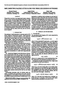
A. Coverage Area Management Service Operation Figs. 2 and 3 show maps in time of the nodes administrative state for a single simulation of the scenario with management. We chose 51 and 181 instants of the simulation time in order to reveal the initial configuration made by the manager and the healing of the configuration after failures, respectively. Fig. 2(a) shows a map of the network in time 51, as seen by the manager. At this time the initial configuration had just finished. As noticed, 18 sensor nodes were chosen to be active. These sensor nodes cover 99.46% of the observation area. The remaining 0.54% are not within the sensing range of any sensor node. It can be observed that the map comprises of only 116 sensor nodes, and not 120 (the total number of nodes). Due to the lost of messages loading nodes coordinates (TRAP-POSITION messages), 4 nodes could not be recognized by the manager. It is interesting to compare this map with the one shown in Fig. 2(b), which presents not the view of the manager, but the view of a global observer. As displayed, the real number of nodes in activity is 32, and not 18. The difference of 14 nodes are due to the lost of 4 TRAP-POSITION messages, as mentioned, summed with the lost of 10 messages loading the command to put the nodes out-of-service (SETOFF messages). Although the lost of SET-OFF messages represented 10.20% from the total sent, it

was still possible to turn 88 redundant nodes off, thus allowing a lot of energy savings. [Figure 2 about here.] Fig. 3 shows the global view of the network in time 181. By this time 32 nodes had exhausted their energy supply. As noticed, these nodes are exactly the ones which took part of the initial virtual topology as shown in Fig. 2(b). It is also observed that in time 181 other 19 nodes took part of the minimum set. These nodes cover 98.08% of the observation area. The other 1.92% was not in the range of observation of any sensor node and hence remained uncovered. [Figure 3 about here.]

B. Scenarios Performance For the purpose of measuring and comparing the performance of each scenario, we elected some metrics, which are:

•

Coverage. Portion of the interest points (in percentage) for which report data were produced in a time period. A coverage of 100% means that the sink node received the temperature values for every interest point inside the observation area.

•

Redundant data. Quantity of redundant data reports received by the sink node. Redundant data reports are measurements of an interest point that have already been sent by other sensor node referring to the same time period. By looking at this metric value one can derive the redundancy level of the network. The higher the redundancy level is, the higher is the sensing application network load, and the higher is the traffic in the network.

•

Delay. Difference in time between the sending an receiving time of a data report, measuring it end-to-end between sensor and sink node.

•

Data report. Quantity of data reports received by the sink node. It includes the redundant data reports.

•

Application messages. Quantity of the temperature monitoring application messages sent in the network.

•

Management messages. Quantity of management messages sent in the network.

Fig. 4 presents the coverage obtained for each scenario. The plot considers the average of the 33 simulations and refers to report data received in each time period (one period is equivalent to 10s of simulation). The results show the coverage in the view of the sink node and thus demonstrate the sensing QoS as perceived by the network observer. The curve exhibited for the unmanaged WSN shows that until the end of the 17th period the coverage value is almost 100% (it is not exactly 100% because there is a part of the area which can not be observed by any sensor, as mentioned in Section VI-A). In the middle of the 18th period, the network perishes completely. This is due to the facts that we the sensor nodes began with equal energy budget and that the application implies the same consumption behavior. The curve for the managed WSN, until the end of the 17th period exhibits similar behavior. As noticed, the coverage value is practically identical. The small degradation (near 0.30%) is mainly an effect of the reduction of the network redundancy. Since the number of data reports transmissions

related to the same interest point is diminished, the probability that a data report becomes lost is higher. If the application in question has a critic area coverage, a decrease in the theoretical sensing range in the virtual topology calculation would diminish this degradation. It is perceived that the first set of sensor nodes in activity tends to have their energy supply exhausted a bit before the end of the unmanaged WSN lifetime (almost 5 s). This happens because the management application causes the sensor nodes to consume energy with management tasks – basically the transmission of TRAP-INITIAL messages and the increase in the transmission time of the data report packet (since the energy value is included). Nevertheless, the manager succeeds quickly in healing the network by reactivating backup nodes, thus preventing a great coverage breach. After the 18th time period, any coverage obtained can be considered a profit, since the unmanaged WSN was not able to provide any coverage beyond this point. It is observed that until the end of the 27th time period the coverage gain is excellent, having a smooth decay until the 44th time period and a strong decay lately. We notice, therefore, that the coverage area management service can help improve the network lifetime significantly, although we could not quantify the benefits, since the coverage level taken as a satisfactory minimum changes from application to application, i.e., depends on the network targets. [Figure 4 about here.] Table III presents the results in relation to redundant data, report data, and delay, for both scenarios. The measurements were conducted during the network start until the time when the first sensor node in the unmanaged WSN stops producing. Thus, the values shown in Table III represent the behavior for both scenarios in a time period without any node failure. The confidence interval of the values is 95%. [Table 3 about here.]

The results shown in Table III prove that the use of the coverage area management service can actually help diminish redundancy. If we analyze the volume of redundant data sent, there was a reduction of 99.25%. This result is a function of the reduction on the quantity of data report messages transmitted (near 76.58%). Nevertheless, the results suggest that the management introduction has a disadvantage. It can be noticed that the delay is increased in approximately 33.22%. Unfortunately, the management services and functions generate an extra traffic that competes with the temperature monitoring application traffic. This was not an intuitive result since, as mentioned, the management helps reducing the application traffic and so the overall traffic. The main reason is that the management traffic flows from base-station to network, and not the opposite as the application traffic. A message flowing in opposite direction is harder to compete with. Other reasons for the increase in the delay include the fact that data report packets are longer in the managed WSN and that the management traffic volume is significant in both directions (base-station to network and also network to application) etc. Table IV presents the quantity of messages transmitted in the scenario with management during the whole network lifetime. The values are also within a 95% confidence interval. It compares management and application traffic volumes. As noticed, the management application inserts a great quantity of messages in the network traffic in order to conclude its tasks. This is also a contributing factor for the small degradation in coverage in the first moments of the network existence and also a significant increase in the delay, when compared to the scenario without management. [Table 4 about here.] The obtained results allow us to conclude that the use of management can bring significant benefits to the network lifetime. Although management services and functions rely on the introduction of new messages in the network or the alteration of old ones, definitely we could not identify any

negative impact that could hinder its utilization, at least for applications similar to the one considered in this work.

VII. C ONCLUSIONS Wireless Sensor Networks (WSNs) have emerged as a solution for several applications. Many research steps, tough, have to be taken in order for the WSNs to be practical and have a commercial appeal. The available sensor node architecture has still strong restrictions, what provokes the simple task of sensing and reporting to be a huge set of efficiency problems. Since these networks will be deployed in regions of hard (or impossible) physical access and the network will have to operate independently from any human interference, management will play a fundamental role. WSNs will have to manage themselves, executing self-maintenance functions in order to satisfy the required QoS, even under failure circumstances. In this work we propose a self-management service for maintaining the desired coverage area level. Area coverage is one of the most important QoS parameters in WSNs. If the sensor nodes do not sense and report back the environment data as supposed or the area coverage is guaranteed only for a small operation time, the network loses its purpose. The service proposed in this work tackles this problem through automatic functions. Besides satisfying coverage area needs, it helps prolonging the network lifetime. The main advantage of our solution is that it can be integrated to other management services as part of a WSN self-management architecture. It is not enough to propose and consider isolated solutions for particular problems in WSNs. We need to design the network considering its many aspects and propose integrated solutions. From the point of view of network management, the coverage management service proposed in this work goes toward this direction. Although in this work we take important steps towards having a complete self-management

solution for WSNs, there are still open issues when coverage area management is concerned. For instance, management functions need to be more flexible (more adaptable to application requirements and network dynamic properties), more efficient (imply lower energy and traffic cost) and more fault-tolerant (worried about every possible type of failure). Also, the use of rather different solutions should be analyzed, mostly in the context of distributed management, different WSN configurations (such as multi-hop networks), different WSN types (such as event-driven networks), and different sensing observation patterns.

ACKNOWLEDGMENTS The development and studies described in this article were completed as part of Sensornet Project (http://www.sensornet.dcc.ufmg.br), funded by CNPq/Ministry of Science and Technology/Brazil (Scientific and Technological Development Council). Some scholarships were given by CAPES/Ministry of Education/Brazil (Foundation Coordination for the Improvement of Higher Education Personnel).

R EFERENCES [1] I. Akyildiz, W. Su, Y. Sankarasubramaniam, and E. Cayirci, “A survey on sensor networks,” IEEE Communications Magazine, vol. 40, no. 8, pp. 102–114, 2002. [2] D. Estrin, R. Govindan, and J. Heidemann, “Embedding the Internet,” Communications of the ACM, vol. 43, no. 5, pp. 39–41, May 2000, special issue guest editors. [3] L. B. Ruiz, J. M. S. Nogueira, and A. A. F. Loureiro, “MANNA: A management architecture for wireless sensor networks,” IEEE Communications Magazine, vol. 41, no. 2, pp. 116–125, 2003. [4] W. Heinzelman, J. Kulik, and H. Balakrishnan, “Adaptive protocols for information dissemination in wireless sensor networks,” in Proceedings of the 5th ACM/IEEE International Conference on Mobile Computing and Networking (MOBICOM’99), Seattle, WA, USA, 1999, pp. 174–185.

[5] D. Tian and N. D. Georganas, “A coverage-preserving node scheduling scheme for large wireless sensor networks,” in Proceedings of the 1st ACM International Workshop on Wireless Sensor Networks and Applications (WSNA’02). Atlanta, GA, USA: ACM Press, 2002, pp. 32–41. [6] R. Wattenhofer, L. Li, P. Bahl, and Y.-M. Wang, “Distributed topology control for wireless multihop ad-hoc networks,” in Proceedings of the 20th IEEE Annual Conference on Computer Communications (INFOCOM’01), 2001, pp. 1388–1397. [7] S. Meguerdichian and M. Potkonjak, “Low power 0/1 coverage and scheduling techniques in sensor networks,” UCLA Technical Reports 030001, 2003. [8] S. Slijepcevic and M. Potkonjak, “Power efficient organization of wireless sensor networks,” in Proceedings of the IEEE International Conference on Communications (ICC’01), vol. 2, Helsinki, Finland, 2001, pp. 472–476. [9] L. B. Ruiz, I. G. Siqueira, L. B. e Oliveira, H. C. Wong, J. M. S. Nogueira, and A. A. F. Loureiro, “Fault management in event-driven wireless sensor networks,” in Proceedings of the 7th ACM/IEEE International Symposium on Modeling, Analysis and Simulation of Wireless and Mobile Systems (MSWIM’04), Venice, Italy, October 2004. [10] J. Staddon, D. Balfanz, and G. Durfee, “Efficient tracing of failed nodes in sensor networks,” in Proceedings of the 1st ACM International Workshop on Wireless Sensor Networks and Applications (WSNA’02). Atlanta, GA, USA: ACM Press, 2002, pp. 122–130. [11] M. R. Garey and D. S. Johnson, Computers and Intractability: A Guide to the Theory of Np-Completeness. New York, NY, USA: W. H. Freeman & Co., 1979. [12] “UCB/LBNL/VINT network simulator (ns-2),” April 1999, available at http://www.isi.edu/nsnam/ns. [13] MICA Wireless Measurement System, Crossbow Technology Inc., 2003, document Part Number: 6020-0041-01. Available at http://www.xbow.com. [14] G. J. Pottie and W. J. Kaiser, “Wireless integrated network sensors,” Communications of the ACM, vol. 43, no. 5, pp. 51–58, 2000.

L IST 1 2 3 4

OF

F IGURES

Example of area division according to sensing . . . . . . . . Nodes administrative state in time 51 . . . . . . . . . . . . . Nodes administrative state in time 181 (global observer view) Coverage in function of the network lifetime . . . . . . . . .

. . . .

. . . .

. . . .

. . . .

. . . .

. . . .

. . . .

. . . .

. . . .

. . . .

. . . .

. . . .

. . . .

28 29 30 31

Fig. 1.

Example of area division according to sensing

50

50

40

40

35

35

30

30

25

25

20

20

15

15

10

10

5

5

0

0 0

5

10

15

20

25 30 X position

35

40

45

50

(a) Manager view Fig. 2.

out−of−service in activity 45

Y position

Y position

out−of−service in activity 45

Nodes administrative state in time 51

0

5

10

15

20

25 30 X position

35

40

45

(b) Global observer view

50

50 out−of−service in activity dead

45 40 35

Y position

30 25 20 15 10 5 0 0

5

10

15

20

25

30

35

40

45

X position

Fig. 3.

Nodes administrative state in time 181 (global observer view)

50

100

unmanaged WSN managed WSN

Coverage (%)

80

60

40

20

0 10

20

30

40

50

60

Time period

Fig. 4.

Coverage in function of the network lifetime

70

80

90

100

L IST I II III IV

OF

TABLES

Network parameters . . . . . . . . . . . . . . . . . . . . . Timing parameters . . . . . . . . . . . . . . . . . . . . . . Results for the time period without sensor nodes failures . Messages transmitted in the managed WSN . . . . . . . .

. . . .

. . . .

. . . .

. . . .

. . . .

. . . .

. . . .

. . . .

. . . .

. . . .

. . . .

. . . .

. . . .

. . . .

. . . .

33 34 35 36

TABLE I N ETWORK PARAMETERS Parameter

Value

Number of nodes Observation area size Network type

120 50 m × 50 m Hierarchical and heterogeneous Follows an uniform distribution 1 Joule

Topology Initial energy (sensor nodes) Initial energy (cluster-head nodes) MAC Protocol Routing algorithm Bandwidth Radio propagation model Transmission power (sensor nodes) Transmission power (cluster-head nodes) Sensing range Energy consumed for communication (sensor nodes) Energy consumed for communication (clusterhead nodes) Energy consumed by cluster-head or sensor nodes in activity Node mobility

100 Joules IEEE 802.11 None (single-hop communication) 100 kbits/s TwoRayGround 5.064 mW (resulting range of 30.5 m) 0.282 W (resulting range of 140 m) 10 m 0.036 W (tx) and 0.005 W (rx) 1.176 W (tx) and 0.588 W (rx) 0.002 mJ

None

TABLE II T IMING PARAMETERS Element type

Sensor node

Cluster-head node

Sink node

Parameter

Value

Start time (uniform distribution) Transmission time of location coordinates Transmission time of the first report data Time interval between successive collected data transmissions Time period to stay out-of-service after a command Start time (uniform distribution) Transmission time of the first TRAP-INITIAL Time interval between successive TRAP-INITIAL transmissions Transmission time of the first aggregated data Time interval between successive aggregated data transmissions Time Interval between successive availability tests Timeout to wait for a data report of a sensor node after reactivating it

Between 5 and 10 s 10 s after start time 40 s after start time 10 s 10 s Between 0 and 5 s 12 s after start time 10 s 52 s after start time 10 s 1s 40 s

TABLE III R ESULTS FOR THE TIME PERIOD WITHOUT SENSOR NODES FAILURES Metric

Unmanaged WSN

Managed WSN

Redundant data Data report Delay

29,568.373 ± 220.676 1,679.879 ± 0.122 3.254 ± 0.181

4,949.529 ± 421.894 393.454 ± 22.710 4.335 ± 0.217

TABLE IV M ESSAGES TRANSMITTED IN THE MANAGED WSN Metric

Value

Application messages Management messages

6,696.909 ± 9.029 5,700.303 ± 62.470