LIFETIME ANALYSIS FOR WIRELESS SENSOR NETWORKS

A THESIS SUBMITTED TO THE GRADUATE SCHOOL OF NATURAL AND APPLIED SCIENCES OF THE MIDDLE EAST TECHNICAL UNIVERSITY

BY

BİLAL ÖĞÜNLÜ

IN PARTIAL FULFILLMENT OF THE REQUIREMENTS FOR THE DEGREE OF MASTER OF SCIENCE IN ELECTRICAL AND ELECTRONICS ENGINEERING

AUGUST 2004

Approval of the Graduate School of Natural and Applied Sciences.

__________________________ Prof. Dr. Canan Özgen Director

I certify that this thesis satisfies all the requirements as a thesis for the degree of Master of Science.

__________________________ Prof. Dr. Mübeccel Demirekler Head of Department This is to certify that we have read this thesis and that in our opinion it is fully adequate, in scope and quality, as a thesis for the degree of Master of Science.

_______________________________ Asst. Prof. Dr. Cüneyt F. Bazlamaçcı Supervisor

Examining Committee Members

(METU – EE)

____________________

Asst. Prof. Dr. Cüneyt F. Bazlamaçcı (METU – EE)

____________________

Prof. Dr. Semih Bilgen

(METU – EE)

____________________

Prof. Dr. Buyurman Baykal

(METU – EE)

____________________

Dr. Altan Koçyiğit

(METU – I I)

____________________

Prof. Dr. Hasan Güran

I hereby declare that all information in this document has been obtained and presented in accordance with academic rules and ethical conduct. I also declare that, as required by these rules and conduct, I have fully cited and referenced all material and results that are not original to this work.

Name, Last name

:

Signature

:

III

Bilal Öğünlü

ABSTRACT LIFETIME ANALYSIS FOR WIRELESS SENSOR NETWORKS Öğünlü, Bilal M.S., Department of Electrical and Electronics Engineering Supervisor: Asst. Prof. Dr. Cüneyt F. Bazlamaçcı August 2004, 79 pages Sensor technologies are vital today in gathering information about certain environments and wireless sensor networks are getting more widespread use everyday. These networks are characterized by a number of sensor nodes deployed in the field for the observation of some phenomena. Due to the limited battery capacity in sensor nodes, energy efficiency is a major and challenging problem in such powerconstrained networks. Some of the network design parameters have a direct impact on the network’s lifetime. These parameters have to be chosen in such a way that the network use its energy resources efficiently. This thesis studies these parameters that should be selected according to certain trade offs with respect to the network’s lifetime. In this work, these trade offs have been investigated and illustrated in detail in various combinations. To achieve this goal, a special simulation tool has been designed and implemented in this work that helps in analyzing the effects of the selected parameters on sensor network’s lifetime. OMNeT++, a discrete event simulator, provides the framework for the sensor network simulator’s development. Ultimately, results of extensive computational tests are presented, which may be helpful in guiding the sensor network designers in optimally selecting the network parameters for prolonged lifetime. Keywords: Wireless Sensor Networks, Energy Efficiency, Network Lifetime, Network Simulation, OMNeT++.

IV

ÖZ TELSİZ ALGILAYICI AĞLARIN YAŞAM SÜRESİ ANALİZİ Öğünlü, Bilal Yüksek Lisans Tezi, Elektrik ve Elektronik Mühendisliği Bölümü Tez Yöneticisi: Yrd. Doç. Dr. Cüneyt F. Bazlamaçcı Ağustos 2004, 79 sayfa Algılayıcı teknolojileri, belli bir ortam ile ilgili bilgi toplama konusunda yaşamsal öneme sahiptir ve telsiz algılayıcı ağların kullanımı gün geçtikçe daha da yaygınlaşmaktadır. Bu ağlar, birtakım çevresel olayları gözlemek amacı ile sahaya yerleştirilmiş belli sayıdaki algılayıcı modülden oluşur. Bu tür enerji kısıtı bulunan ağlarda, enerji verimliliği konusu, algılayıcı modüllerdeki sınırlı batarya kapasitesi nedeni ile çözülmesi gereken temel bir problemdir. Bazı ağ tasarım parametreleri ağın yaşam süresi üzerinde doğrudan bir etkiye sahiptirler. Bu parametreler, ağın kendi enerji kaynaklarını verimli olarak kullanmasını sağlayacak şekilde seçilmelidir. Bu tez, telsiz algılayıcı ağların yaşam süresi göz önüne alınarak ortaya konan belli dengelere göre seçilmesi gereken parametreler üzerinde yapılan bir çalışmayı içermektedir. Bu çalışmada, tüm bu dengeler, birçok kombinasyon göz önüne alınarak, detaylı bir şekilde incelenmiş ve açıklanmıştır. Bu amaca yönelik olarak, seçilen parametrelerin algılayıcı ağların yaşam süresi üzerine etkilerini inceleme konusuna yardımcı olacak özel bir simülasyon modeli tasarlanmış ve bu çalışmaya uygulanmıştır. Bir kesikli olay simülatörü olan OMNeT++, bahsi geçen bu algılayıcı ağlarının tasarlanması amacı ile bir çatı sunmaktadır. Sonuç olarak, ağın yaşam süresini uzatmak için, ağ parametrelerini optimum seçme durumunda olan tasarımcıya yol göstermede yardımcı olabilecek geniş sayıda sayısal testin sonuçları sunulmuştur.

V

Anahtar Sözcükler: Telsiz Algılayıcı Ağlar, Enerji Verimliliği, Ağ Yaşam Süresi, Ağ Simülasyonu, OMNeT++.

VI

To my loving MOTHER.

VII

ACKNOWLEDGEMENTS First and foremost, I express my sincere gratitude to my advisor of two years, Asst. Prof. Dr. Cüneyt F. Bazlamaçcı, for his supportive guidance and constructive criticism throughout this study.

My family have also been very supportive, not just during this study, but throughout my entire life. Their love provided me with the motivation and endeavor to accomplish this piece of work. They have always been a great source of encouragement and support. I especially want to thank them for instilling in me the many values that have become so important to me. They gave me so much that I can never pay them back. I will owe them gratitude and thankfulness forever.

Finally, I would like to thank everyone else who has supported me in one way or another throughout this study.

VIII

TABLE OF CONTENTS

ABSTRACT ........................................................................................................................................... IV ÖZ..............................................................................................................................................................V ACKNOWLEDGEMENTS...............................................................................................................VIII TABLE OF CONTENTS...................................................................................................................... IX LIST OF FIGURES .............................................................................................................................. XI LIST OF TABLES .............................................................................................................................. XII LIST OF ABBREVIATIONS ...........................................................................................................XIII 1. INTRODUCTION............................................................................................................................... 1 2. WIRELESS SENSOR NETWORKS: BACKGROUND AND RELATED WORK................... 6 2.1. MOTIVATION ......................................................................................................................... 6 2.1.1. History............................................................................................................................... 6 2.1.2. Current Trends.................................................................................................................. 7 2.1.3. Challenges....................................................................................................................... 10 2.2. ISSUES IN WIRELESS SENSOR NETWORKS .................................................................. 11 2.2.1. Characteristics of a Wireless Sensor.............................................................................. 11 2.2.2. An Application Example: Environmental Data Collection............................................ 12 2.2.3. Energy Model.................................................................................................................. 14 2.2.4. Data Aggregation............................................................................................................ 15 2.2.5. Reactive and Proactive Networks................................................................................... 17 2.2.6. Communication ............................................................................................................... 17 2.2.7. Network Layer and Routing............................................................................................ 18 2.3. SYSTEM PARAMETERS ..................................................................................................... 19 2.3.1. Time-Varying Node Density ........................................................................................... 19 2.3.2. Battery Capacity ............................................................................................................. 19 2.3.3. Communication and Sensing Ranges ............................................................................. 20 2.3.4. Query Period................................................................................................................... 20 2.3.5. Utility............................................................................................................................... 21 2.3.6. Lifetime............................................................................................................................ 21 3. PROBLEM DEFINITION ............................................................................................................... 22 3.1. 3.2. 3.3. 3.4.

PROBLEM STATEMENT ..................................................................................................... 23 SOLUTION APPROACH AND NETWORK CONFIGURATION ..................................... 24 CONSTRAINTS ..................................................................................................................... 25 REQUIREMENTS AND ASSUMPTIONS ........................................................................... 27

4. DESIGN AND IMPLEMENTATION OF A SENSOR NETWORK SIMULATION EXPERIMENT...................................................................................................................................... 29 4.1. 4.2.

WHAT IS OMNET++?........................................................................................................... 29 THE SIMULATION IMPLEMENTATION .......................................................................... 31

IX

5. SIMULATION STUDY.................................................................................................................... 40 6. CONCLUSION.................................................................................................................................. 56 REFERENCES ...................................................................................................................................... 61 APPENDIX A: USER MANUAL FOR THE SIMULATION AND ANALYSIS TOOL............. 63 APPENDIX B: THE SPECIFIC SOURCE CODES......................................................................... 66 APPENDIX C: THE RESULT SHEET.............................................................................................. 71

X

LIST OF FIGURES

Figure 1. A snapshot of the simulation ............................................................................................... 34 Figure 2. A snapshot of the simulation when the nodes set their connections ............................... 35 Figure 3. Two snapshots of the gates, first one is used for only connection but the second one is used for both connection and routing purposes. .............................................................. 36 Figure 4. Two snapshots of the messages, first one is inter-nodal message and second one is intra-nodal message ............................................................................................................. 36 Figure 5. Two snapshots of the sensor nodes, first one just generated the message but second one is about to send it.................................................................................................................. 37 Figure 6. A snapshot of the user interface of the simulation............................................................ 38 Figure 7. Lifetime of the Network vs. Communication Radius - 1.................................................. 41 Figure 8. Lifetime of the Network vs. Communication Radius -2................................................... 42 Figure 9. Lifetime of the Network vs. Communication Radius - 3.................................................. 43 Figure 10. Lifetime of the Network vs. Query Period....................................................................... 44 Figure 11. Lifetime of the Network vs. Node Density - 1.................................................................. 45 Figure 12. Lifetime of the Network vs. Node Density – 2 ................................................................. 46 Figure 13. Lifetime of the Network vs. Node Density - 3.................................................................. 47 Figure 14. Lifetime of the Network vs. Communication Radius - 4................................................ 48 Figure 15. Lifetime of the Network vs. Communication Radius - 5................................................ 49 Figure 16. Lifetime of the Network vs. Communication Radius - 6................................................ 50 Figure 17. Lifetime of the Network vs. Communication Radius -7................................................. 51 Figure 18. Lifetime of the Network vs. Node Density - 4.................................................................. 52 Figure 19. Lifetime of the Network vs. Node Density - 5.................................................................. 53 Figure 20. Lifetime of the Network vs. Node Density - 6.................................................................. 54 Figure 21. The user interface of the Excel file ................................................................................... 64

XI

LIST OF TABLES

Table 1.

The parameters and their selected values……………………………32

Table C.1. The Result Sheet……………………………………………………….72

XII

LIST OF ABBREVIATIONS

CMOS

:

Complementary Metal Oxide Semiconductor

CPU

:

Central Processing Unit

ID

:

Identity

Kb

:

Kilobit(s)

KB

:

KiloByte(s)

MAC

:

Medium Access Control

MANET

:

Mobile Adhoc NETwork

ME

:

Minimum Energy

MH

:

Minimum Hop

MIPS

:

Million Instructions Per Second

MSVC

:

MicroSoft Visual C

OMNeT++

:

Objective Modular Network Testbed in C++

PDA

:

Personal Digital Assistance

QoS

:

Quality of Service

RF

:

Radio Frequency

TDMA

:

Time Division Multiple Access

WSN

:

Wireless Sensor Network

W

:

Watt

WWW

:

World Wide Web

XIII

CHAPTER 1 INTRODUCTION

In the near future, the improvements in digital circuit technology will allow the integration of functionalities for information gathering, processing, and communication in tight packaging, perhaps even on a single chip. Information gathering functionalities are performed by the actual sensors, e.g., devices to measure temperature, air pollution, pressure, etc. Information processing functionalities rely essentially on processing units like microprocessors or microcontrollers, memory, and their interconnection. Information communication functionalities are performed by wireless communication devices, typically communicating in the radio spectrum, sometimes visible or infrared light being other options. Finally, some other support functionalities like power supply, etc., are required to build a complete sensor node. It is envisioned that, in future, wireless sensor networks will be an integral part of our lives. Sensor nodes can be used for continuous sensing, event detection, location sensing, and local control of actuators. The concepts of micro-sensing and wireless connection of these nodes promise many new application areas. Some application categories are military, environment, health, home and other commercial areas. A sensor network is composed of a number of sensor nodes, which are densely deployed either inside the phenomenon area or very close to it. The position of sensor nodes need not be engineered or pre-determined. This allows random deployment in inaccessible terrain or disaster relief operations. On the other hand, this also means that sensor network protocols and algorithms must possess selforganizing capabilities.

1

After deployment, these nodes are generally stationary and self-organized into a network to gather information and send it to the control center where end-user can retrieve the data. In essence, sensor networks will provide the end user with intelligence and a better understanding of the environment. Another unique feature of sensor networks is the cooperative effort of sensor nodes. While the capabilities of any single device are minimal, the composition of hundreds of devices offers radical new technological possibilities. The power of wireless sensor networks lies in the ability to deploy large numbers of tiny devices that assemble and configure themselves as network nodes. Unlike traditional wired systems, deployment costs would be minimal. Instead of having to deploy wires through protective conduits, installers simply have to place small size devices at the territory. The network could be incrementally extended by simply adding more devices – no rework or complex reconfiguration. Generally, when people consider wireless devices they think of items such as cell phones, personal digital assistance (PDA), or laptops. These items cost hundreds of dollars, target specialized applications, and rely on the pre-deployment of extensive infrastructure support. In contrast, wireless sensor networks use small, lowcost embedded devices for a wide range of applications and do not rely on preexisting infrastructure. The vision is that such a device will cost less than $1 by 2010. Unlike traditional wireless devices, wireless sensor nodes do not need to communicate directly with the nearest high power control center, but only with their neighbors. Instead of relying on a pre-deployed infrastructure, each individual sensor becomes part of the overall infrastructure. Peer-to-peer networking protocols provide a mesh-like interconnect to shuttle data between the many of tiny embedded devices in a multi-hop fashion. The envisioned flexible mesh architectures dynamically adapt to support introduction of new nodes or expand to cover a large geographic region. Additionally, the system can automatically adapt to compensate for node failures.

2

Since sensor nodes are densely deployed, neighbor nodes may be very close to each other. Hence, multihop communication in sensor networks is expected to consume less power than the traditional single hop communication. Furthermore, the transmission power levels can be kept low, which is highly desired in covert operations. Multihop communication can also effectively overcome some of the signal propagation effects experienced in long-distance wireless communication. One of the most important constraints on sensor nodes is the low power consumption requirement. Sensor nodes carry limited, generally irreplaceable, power supplies. Many sensors may be deployed with non-rechargeable batteries. Since the sensor nodes will die one by one during the operation of the network, all the network requirements must be met with minimum power consumption due to battery limitations and, for many applications, the inability to recharge these batteries. In sensor networks, a decrease in the number of available sensor nodes can deeply degrade the network performance, due to either some areas being not monitored or some data being not transferred through the network. Furthermore, it may be infeasible to replace thousands of nodes in hostile or remote regions. Therefore, while traditional networks aim to achieve high quality of service (QoS) provisions, sensor network protocols must focus primarily on power conservation. They must have inbuilt trade-off mechanisms that give the end user the option of prolonging network lifetime at the cost of lower throughput or higher transmission delay. Many researchers are currently engaged in developing schemes that fulfill these requirements. In this study, we describe a simplified architecture for self-organizing wireless sensor networks. A wireless sensor network of the type investigated here refers to a group of sensors, or nodes, deployed randomly over a defined terrain. These sensor nodes are capable of sensing specific information within their sensing range. The nodes are linked by a wireless medium to perform distributed sensing tasks. Connections between nodes are formed using radio communications. The ultimate aim of a node is actually to send the information that it gathers locally to the

3

destination, which is called the user node. While doing that, the main concern is to consume energy in an optimum way. Our claim is that significant reductions in energy consumption can be achieved if wireless sensor networks are designed specifically with minimum energy consumption requirement in mind. In order to maximize the lifetime of a wireless sensor network, we must minimize the energy consumption within the entire network. The way sensor networks are organized internally plays an important role in decreasing the energy budget to perform certain functions, and therefore proper design of the sensor network architecture is an important goal to be pursued. There are several parameters mainly related to the network lifetime. These are initial battery capacity, communication radius, query period and node density. These parameters have certain trade offs in terms of the lifetime and therefore the relations between these parameters should be investigated to support our claim. In this study, after the description of these relations, we illustrate the trade offs by various combinations of the sensor network parameter values. A simulation tool, which helps in analyzing the effects of the parameters on sensor network lifetime is designed for this purpose and implemented by means of a discrete event simulator environment, OMNeT++. The thesis is organized as follows: Chapter 2, “Wireless Sensor Networks: Background and Related Work”, explains in detail what a wireless sensor network is and emphasizes the key concepts and some system parameters in sequence. A literature survey on past studies on these concepts is also presented. Chapter 3, “Problem Definition”, describes what the problem solved in this thesis is and gives detailed information about our approach. Constraints, limitations and assumptions are all addressed in this chapter.

4

Chapter 4, “Design and Implementation of a Sensor Network Simulation Experiment”, presents the development of the simulation tool. OMNeT++, a discrete event simulator environment is used as the framework for this purpose. Although our simulation study aims to evaluate the trade offs between the network parameters that affect the lifetime, the developed simulator can be modified and extended to be used for various other sensor network related purposes. Chapter 5, “Simulation Study”, explains the work environment necessary for collecting the arranged results and also includes plots and their analysis. Chapter 6, “Conclusions”, summarizes the findings and contributions of this study and outlines possible directions for future research. At the end, the result tables and the graphics are illustrated in the appendices. In addition, the algorithms designed are presented as C++ code and the user manuals for the simulation tool and the designer guide interface are all included in the appendices.

5

CHAPTER 2 WIRELESS SENSOR NETWORKS: BACKGROUND AND RELATED WORK

2.1. MOTIVATION

2.1.1. History

Since the first wireless digital network, ALOHANET, debut in 1971 at the University of Hawaii, wireless networks have experienced explosive growth in mobile and personal communications. Wireless networks provide users with extended computing capabilities and mobility. The existing wireless networks are classified into two categories: infrastructure and ad hoc networks [1]. The infrastructure network architecture contains a wired backbone, which connects to a special switching node called base station. Communication between hosts has to go through the base station. An ad hoc network on the other hand, is a self-organizing system consisting of hosts that do not rely on the presence of any fixed network infrastructure. A cellular network belongs to the first type and a mobile ad hoc network (MANET) belongs to the second type. Recently a number of short-range wireless networking systems have been developed. Bluetooth intends to replace the wire and provides RF connection between devices. It is a star network where a master node is able to have up to seven active slave nodes attached to it to form a piconet. The time-division multiple access (TDMA) schedule

6

is centrally assigned, and all nodes are synchronized to the master in this system. Another commercial short-range system, HomeRF, is a single-hop ad hoc network. In contrast to all these networks, the emerging wireless sensor networks, simply sensor networks, are new family of networks. Sensor networks normally comprise of many nodes. After deployment, these nodes are generally stationary and self-organized into a network to perform a higher-level sensing task. Within a sensor network, wireless sensor nodes gather acoustic, magnetic, or seismic information and send the information to a control center or base station, where the end-user can retrieve the data. The emergence of wireless sensor networks requires a new wireless system design paradigm. Although similar to traditional personal communications networks and wireless data networks in some respects, wireless sensor networks need to function in a fundamentally different manner since they are carrying out a very different task than cell phones, pagers, and Bluetooth wireless network interface cards. The increased dynamic nature of the network means that previously used personal communication network system design techniques will not necessarily produce adequate solutions. The data flow in wireless sensor networks is controlled by a new generation of protocols, designed to handle the data rates and quantities generated by the sensors and to do so using very little power.

2.1.2. Current Trends

Recent advances in wireless communications and electronics have enabled the development of low-cost, low-power, multifunctional sensor nodes that are small in size and communicate in short distances. These tiny sensor nodes, which consist of sensing, data processing, and communicating components, leverage the idea of sensor networks.

7

Sensor networks represent a significant improvement over traditional sensors, which are deployed in the following two ways [2]: ™

Sensors can be positioned far from the actual phenomenon, i.e., something

known by sense perception. In this approach, large sensors that use some complex techniques to distinguish the targets from environmental noise are required. ™

Several sensors that perform only sensing can be deployed. The positions of

the sensors and communications topology are carefully engineered. They transmit time series of the sensed phenomenon to the central nodes where computations are performed and data are fused. In some application scenarios, replenishment of power resources might be impossible. Sensor node lifetime, therefore, shows a strong dependence on battery lifetime. In a multihop sensor network, each node plays the dual role of data originator and data router. The disfunctioning of few nodes can cause significant topological changes and might require re-routing of packets. Hence, power conservation and power management take on additional importance. It is for these reasons that researchers are currently focusing on the design of power-aware protocols and algorithms for sensor networks. In other mobile and ad hoc networks, power consumption has been an important design factor, but not the primary consideration, simply because power resources can be replaced by the user. The emphasis is more on QoS provisioning than the power efficiency. In sensor networks though, power efficiency is an important performance metric, directly influencing the network lifetime. Application specific protocols can be designed by appropriately trading off other performance metrics such as utility with power efficiency. Sensor networks may consist of many different types of sensors such as seismic, low sampling rate magnetic, thermal, visual, infrared, acoustic and radar, which are able to monitor a wide variety of ambient conditions that include the following [3]:

8

™

Temperature,

™

Humidity,

™

Vehicular movement,

™

Lightning condition,

™

Pressure,

™

Soil makeup,

™

Noise levels,

™

The presence or absence of certain kinds of objects,

™

Mechanical stress levels on attached objects, and

™

The characteristics such as speed, direction, and size of an object. These are some of the proposed applications found in the literature for

wireless sensor networks, but by no means are they the only ones. One of the attractive features of this technology is the potentially large number of areas to which it can be applied. Realization of these and other sensor network applications require wireless ad hoc networking techniques. Although many protocols and algorithms have been proposed for traditional wireless ad hoc networks, they are not well suited for the unique features and application requirements of sensor networks. To illustrate this point, the differences between sensor networks and ad hoc networks [4] are outlined below: ™

The number of sensor nodes in a sensor network can be several orders of

magnitude higher than the nodes in an ad hoc network. ™

Sensor nodes are densely deployed.

™

Sensor nodes are prone to failures.

™

The topology of a sensor network changes very frequently.

™

Sensor nodes are limited in power, computational capacities, and memory.

™

Sensor nodes may not have global identification (ID) because of the large

amount of overhead and large number of sensors.

9

2.1.3. Challenges

A sensor network design is influenced by many factors, which include fault tolerance; scalability; production costs; operating environment; sensor network topology; hardware constraints; transmission media; and power consumption. These factors are addressed by many researchers. However, none of these studies have a full-integrated view of all factors that are driving the design of sensor networks and sensor nodes. These factors are important because they serve as a guideline to design a protocol or an algorithm for sensor networks. Unlike traditional well-structured computer networks, where connecting devices to the network using a relatively static network configuration is often cumbersome, sensor networks are unstructured and consist of very large number of sensors. Building self-organizing sensor networks is difficult for the following main reasons: First, many different types of sensors with a range of capabilities may be deployed with different specialized network protocols and application requirements. Datacentric networks, in which data is more important than any other information like the location of the nodes, are becoming common in sensor networks. With many mixed types of sensors and applications, sensor networks may need to support several data-centric network protocols simultaneously. Second, these mixed types of sensor nodes may be deployed incrementally and spontaneously with little or no preplanning. The networks must be extendible to include new types of sensor nodes and services. They must be deployed spontaneously to form efficient ad-hoc networks using sensors with limited computational, storage and short-range wireless communication capabilities. The

10

nodes should then rapidly coordinate with each other to detect, track and report activities and disseminate the information efficiently through the impromptu network of sensors. Third, the sensor network must react rapidly to changes in the sensors composition, task or network requirements, device failure and degradation of sensor nodes. Sensor devices may be deployed in very harsh environment, and subject to destruction and dynamically changing conditions. The configuration of the network will frequently change due to constant changes in reachability of sensors, power availability and task requirements. The network protocols must be survivable in spite of device failures and frequent real-time changes. The sensor network must be secure in the face of this open and dynamic environment. In short, the challenge is to map the overall system requirements down to individual device capabilities, requirements and actions. Critical sensor information must be disseminated through transactions and dynamic query processing modules supported by the appropriate distributed services and network protocols to solve the problems of dispersion, disconnection, dynamic reconfiguration and limited power availability. The underlying principle for building self-organizing sensor networks that can overcome the above challenges is to provide the fundamental mechanisms upon which other networking and system services may be spontaneously specified and reconfigured.

2.2. ISSUES IN WIRELESS SENSOR NETWORKS

2.2.1. Characteristics of a Wireless Sensor

11

The architecture of a sensor node's hardware consists of the usual components like processor, memory, wireless interface, power supply, as well as the sensor devices. An individual sensor device can be either an actual sensor or an actuator (for uniformity, both are referred to as “sensor device”). A single sensor node can contain a single or multiple sensor devices of the same or different types. In principle, a sensor should be able to tell a host the kind of measurements it can make, its range, accuracy, linearization and signal conditioning requirements. Each sensor thus becomes an entire electronic system - complete with transducer, amplifier, analog-todigital converter, microprocessor and lookup table. In brief, the concept of wireless sensor networks is based on a sensor resulting into a simple equation: Sensing + CPU + Radio = Thousands of potential applications [9]. As soon as the capabilities of a wireless sensor network are understood, hundreds of applications spring to mind. It seems like a straightforward combination of modern technology.

2.2.2. An Application Example: Environmental Data Collection

The environmental data collection application is characterized by having a large number of nodes continually sensing and transmitting data back to a set of base stations that store the data using traditional methods. These networks generally require very low data rates and extremely long lifetimes. In a typical usage scenario, the nodes will be evenly distributed over an outdoor environment. The distance between adjacent nodes will be minimal yet the distance across the entire network will be significant.

12

After deployment, the nodes must first discover the topology of the network and estimate optimal routing strategies [7]. The routing strategy can then be used to route data to a central collection point. Environmental data collection applications typically use tree-based routing topologies where each routing tree is rooted at high-capability nodes that sink data. Data is periodically transmitted from child nodes to parent nodes up to the treestructure until it reaches the sink. With tree-based data collection, each node is responsible for forwarding the data of all its descendents. Nodes with a large number of descendants transmit significantly more data than leaf nodes. These nodes can quickly become energy bottlenecks. Once the network is configured, each node periodically samples its sensors and transmits its data up the routing tree towards the base station. The typical environmental parameters being monitored, such as temperature, light intensity, and humidity, does not change quickly enough to require higher reporting rates. In addition to large sample intervals, environmental monitoring applications do not have strict latency requirements. Data samples can be delayed inside the network for moderate periods of time without significantly affecting application performance. In general, the data is collected for future analysis but not for real-time operation. As the network ages, it is expected that nodes will fail over time. Periodically the network will have to reconfigure itself to handle node/link failures or to redistribute network load. The most important characteristics of the environmental monitoring requirements are long lifetime, low data rates and relatively static topologies. Additionally, it is not essential that the data be transmitted in real time back to the

13

central collection point. The data transmission can be delayed inside the network as necessary in order to improve network efficiency.

2.2.3. Energy Model

The main task of a sensor node in a sensor field is to detect events, perform quick local data processing, and then transmit the data. Power consumption can hence be divided into three domains: sensing, data processing and communication. In general, a sensor node may consist of several components. The main components are a sensor, a processor, a radio, a battery, external memory, and peripherals (e.g. a voltage regulator, debugging equipment or peripherals to drive an actuator, etc.). In the presented model, the first four components are considered. The external memory can be neglected in this stage since its use of energy is rather complex and needs an own energy model if the memory is a relevant part of the functional behavior of the sensor node and not only used for storage. The peripherals can also be quite different and, thus, cannot be integrated in an energy model of a sensor node in a uniform way. The usage of energy by the other components is independent of the current energy state of the battery, which implies that the reduction of the energy state of the battery depends only on the actions of these other components. Based on these assumptions, it remains to give models for the energy consumption of the three major components, i.e., the sensor, the processor and the radio. In a wireless sensor network, communication is the major consumer of energy. To better grasp this idea; let us compare energy costs of data transmission via radio and data processing. Taking the example described in [8], for ground-to-ground transmission, it costs 3J of energy to transmit 1Kb of data to a distance of 100m. On the other hand, a general-purpose processor with the modest specification of 100

14

million instructions per second (MIPS)/W processing capability executes 300 million instructions for the same amount of energy. In this section, we present a basic version of an energy model for a sensor node. The aim of the model is to predict the current energy state of the battery of a sensor node based on historical data on the use of the sensor node and the current energy state of the battery. The model most often used for the RF system is the path loss model, in which the received power is Pr = Pt . r -a, where r is the distance between the transmitter and the receiver, a is the distance-power gradient, and has values between 2 and 4, depending on the characteristics of the communication medium, and Pt is the transmitting power. We assume that all nodes have the same power threshold for the signal detection, and we consider this value normalized to one. Therefore, the transmitting power Pt needed to support a link of length r is r a. The energy consumption of a wireless node has two components, i.e. transmitting power and the receiving/processing power. We can consider the transmitting power to be the dominate power consumption factor. We can assume that omni-directional antennas are used, which means that if a node transmits at power level r a, any node within the distance of r of it can receive the signal. The factor a represents signal attenuation and is adjusted depending on the model used. For free space environment a = 2 and for noisy urban environment a = 4 [10]. In a noiseless rural environment a can be taken as 2.

2.2.4. Data Aggregation

Sensor data are different from the data associated with traditional wireless networks in that it is not the actual data itself that is important. Rather, the analysis of

15

data, which allows end-user to determine something about the environment that is being monitored, is the important result of a sensor network. For example, if the sensors are monitoring an area for surveillance purpose, the end-user does not need to see the data from each of the sensors but needs to know if there was an intrusion in the area being monitored. Hence, automated models of combining or aggregating the data into a small set of meaningful information are required. In addition, to help avoid information overload, data aggregation, also known as data fusion, can combine several unreliable data measurements to produce a more accurate signal by enhancing the common signal and reducing the uncorrelated noise. The classification on the aggregated data may be by a human element or be automated. A data aggregation at a routing node is the combination of data from different sources, and can be implemented in a number of ways. The simplest data aggregation function is duplicate suppression. Duplicate suppression is already practiced in commercial wireless messaging networks. Other aggregation functions could be max, min, or any other function with multiple inputs. One of the important benefits of data aggregation is efficiency in energy consumption. The energy gain due to data aggregation can be quite significant particularly when there are many sensor nodes (information sources) that are many hops away from the sink node (user node) [12]. For modeling purposes we can make a simplifying assumption - the aggregation function is such that each intermediate node in the routing transmits a single aggregate packet even if it receives multiple input packets one after another. We will refer to the information received by the sink when it has obtained the messages transmitted by all sources in a given flow (whether or not these messages are aggregated) as a “datum”.

16

2.2.5. Reactive and Proactive Networks

There exist two types of information dissemination in wireless sensor networks. One of them results from a stimulus, the other one occurs once the user has a query. The network in which the former exists is called reactive network. The latter is for a proactive network. Proactive networks only update (send) information that they sense on demand. In contrast, reactive networks update (send) their information by stimuli in the field. For sensor networks that experience greater dynamic changes, reactive routing algorithms are more appropriate, whereas for those that are more static and experience infrequent topological change, proactive routing algorithms are more efficient [5].

2.2.6. Communication

Any sensor node will be equipped with wireless communication devices. The preferred way of communication for the energy efficiency is radio-frequency communication. The radio will be expected to provide simple modem functionality, accepting and delivering a bit-serial stream of a simple serial interface and converting this into a bit-serial stream over the radio interface. In addition, a more advanced radio subsystem is also conceivable that already handles simple frame detection or similar functionality. Either approach can be used in a sensor node with the appropriate modification of the device drivers/physical layer protocols. Important aspects in selecting appropriate devices for a prototype are the ability to perform transmission power control. Low cost, small form factor, and power efficiency will play a major role for future products (and are considered by the manufacturers of the sensor nodes), but play a minor role within the definition of the architecture.

17

2.2.7. Network Layer and Routing

Sensor nodes are scattered densely in a field either close to or inside the phenomenon area. The ad hoc principle does not usually fit the requirements of the sensor. The networking layer of sensor networks is usually designed according to the following principles: ™

Power efficiency is always an important consideration.

™

Sensor networks are mostly data centric.

™

Data aggregation is useful only when it does not hinder the collaborative

effort of the sensor nodes. Having considered the above principles, the following well-known approaches can be used to select an energy efficient route: ™

Minimum energy (ME) route: The route that consumes ME to transmit the

data packets between the sink and the sensor node is the ME route. ™

Minimum hop (MH) route: The route that makes the MH to reach the sink is

preferred. Note that the ME scheme selects the same route as the MH when the same amount of energy is used on every link. Therefore, when nodes broadcast with the same power level without any power control, MH is then equivalent to ME [6].

18

2.3. SYSTEM PARAMETERS

2.3.1. Time-Varying Node Density

In designing a sensor network, a user usually has a fixed cost budget that places an upper bound on the total number of nodes that can be deployed. Furthermore, the physical environment may put a constraint on the number of nodes that can be deployed. Density relates to the number of nodes that have to be deployed in order to achieve the desired objective. If no runtime technique is used, all nodes die approximately at the same time. This is by assuming that all sensor nodes with almost similar initial energy content are deployed at almost the same time and by assuming that they also see similar traffic. In such scenarios, density of the network remains constant at the initial density for certain time and then suddenly drops to zero. However, several cooperative cell-based strategies have been proposed to minimize the energy consumption in a sensor network. These are indeed feasible because in general, sensor networks are envisioned to be dense networks consisting of many nodes. In such scenarios, nodes die at different times and the density of the network decreases in a more uniform manner. Thus, a design recipe must enable one to estimate the lifetime and to tune the parameters to satisfy the user’s needs [5].

2.3.2. Battery Capacity

In wireless sensor networks, replenishment of power resources might be impossible. As time progresses, several nodes die and thus the density of the nodes decreases. The initial energy content of the nodes imposes an upper bound on the

19

network lifetime. Sensor node lifetime, therefore, shows a strong dependence on battery capacity. The aim of the designer must be to predict the current energy state of the battery of a sensor node based on historical data on the use of the sensor node and the initial energy state of the battery.

2.3.3. Communication and Sensing Ranges

A key design parameter for any wireless sensor network is its communication range and sensing range. While there is an argument that the coverage of the network is not limited by the transmission range of the individual nodes, the transmission range does have a significant impact on the minimal acceptable node density. If nodes are placed too far apart it may not be possible to create an interconnected network or one with enough redundancy to maintain a high level of reliability. Most application scenarios have natural node densities that correspond to the granularity of desired sensing level. If the radio communication range demands a higher node density, additional nodes must be added to the system to increase node density to a tolerable level [5].

2.3.4. Query Period

In a data-collecting network, effective sampling rate is a primary parameter. We define the effective sampling rate as the inverse of the query period in which sensor data at each individual sensor can be taken and be communicated to a collection point in a data collection network. Fortunately, environmental data collection applications typically have sampling rates of a few samples per minute.

20

However, in addition to the sampling rate of a single sensor, we must also consider the impact of the multi-hop networking architecture on a node’s ability to relay the data of surrounding nodes effectively.

2.3.5. Utility

The utility in essence represents the overall useful information that can be received by the user. Mathematically, it is defined as the product of probability of connectivity and accuracy [5]. The design problem is quite complex to formulate mathematically but in our simulation study, we have measured utility by using the observed throughput at the user node. Hence our utility interpretation is as follows: Utility = (What I got) / (What I’m expecting)

2.3.6. Lifetime

Finally, a user would be concerned of how long the network can last and deliver. For cases, where the user wants the network to detect objects with a desired accuracy as long as possible, optimizing the lifetime becomes important. For other cases, where the area needs to be monitored only for a fixed period of time, the lifetime is known a priori and thus a user would like the network to be designed for just the required amount of time. The lifetime of the network is then defined as the time where the utility falls below a certain user-defined threshold [5]. This threshold is called the user satisfaction limit.

21

CHAPTER 3 PROBLEM DEFINITION

In Chapter 2, we discussed the various properties of wireless sensor network and sensor nodes. The given properties of the sensor network may vary due to varying conditions in which the network is deployed. Some properties may attenuate due to the effect of others. The wireless sensor network closely resembles an ad hoc network deployment. In these networks, neither the initial configuration of the nodes is known nor the connection between the nodes. When the wireless sensor network is established in an unknown environment, it is quite difficult to set up an efficient network initially. Each node will try to establish a single edge routing path to the sink through the router nodes. In a monitoring type of scenario, data acquired for each sensor node is more important than the source and location of the node. The role of any wireless sensor network is to support the detection notifications, coordinate the signal processing functions and communication protocols under a stringent energy constraint. In a broader sense, a wireless sensor network is formed from the integration of sensing, signal processing, and communication functions.

22

3.1. PROBLEM STATEMENT

The way sensor networks are organized internally may play a role in decreasing the energy budget to perform certain functionalities, and therefore proper design of the sensor architecture is an important goal to be pursued. To maximize the lifetime of the network, we need to minimize the energy dissipation for communication by reducing the number of sensing and receiving operations and reducing the transmission distance. To maximize the lifetime of the network, we need to minimize the energy dissipation in the network by adjusting the energy related parameters of the network. There are several parameters mainly related to the network lifetime. These are initial battery capacity, communication radius, query period and node density. These parameters are thought to have certain trade offs in terms of the lifetime and therefore the relations between these parameters should be thoroughly investigated. The present study aims to describe these relations and find out their trade off characteristics by trying out various parameter combinations. For this purpose, a simulation tool that helps in analyzing the effects of the parameters on sensor network lifetime has been designed and implemented by means of OMNeT++, a discrete event simulator environment [13]. To be able to analyze the results, the simulation can be iterated many times with various parameter combinations. The trade offs between the parameters we are dealing with may vary according to the configuration chosen. Eventually, a user interface collecting the results of the iterations is to be prepared for guiding the sensor network designer in optimally selecting the parameters proposed to improve the lifetime of the network.

23

3.2. SOLUTION APPROACH AND NETWORK CONFIGURATION

In this section, we discuss a method of setting up a network topology for wireless sensor networks and discuss how sensor generated data flows through the network before arriving at the sink node. In this section, also we mention an efficient algorithm called Minimum Hop (MH) Routing Algorithm. The application of MH Routing on wireless sensor networks was discussed in the previous chapter. In order to conserve battery power, it is better to use a reactive and energy efficient routing protocol. The ‘dynamic’ version of the MH Routing Algorithm discussed briefly in the previous chapter is a protocol that determines a minimum hop route only when required. This protocol is more survivable since reactive routing does not have a single point of failure and allow multiple routes between nodes. In the following, the self organizing network formation and the problem solution approach is outlined: A topology implementing MH Routing Algorithm is first constructed. It is a self-configuring wireless topology connecting all nodes and each node has no more than one routing edge which goes out from the node. The constructed topology is a simple realization of the existing wireless network architecture with an emphasis of features exploited by the MH Routing Algorithm. In this work, we aim to simulate a prototype wireless sensor network. Simulating a suitable and application specific wireless network with various control parameters such as initial battery capacity, communication radius, query period, and node density is particularly difficult. Therefore, we have made some assumptions to realize our scenario as a simulation. These assumptions are presented at the end of this chapter.

24

A sensor network is required to be self-configurable when deployed. The major goal of the deployment is to cover the maximum area within which the network functions with ease. There are various different ways that the sensors follow to establish a network. The nodes have to communicate efficiently with their neighbors after the formation of the network. Nodes need to act as both routers and sources. Due to the limited transmission range, communication has to be performed over multiple hop paths. All active nodes sense data. Among them, some nodes also act as relay nodes to relay data to the user node. The nodes have the following properties: ™

The user node is fixed and has sufficient power supply; also, it has no energy

constraints. ™

All sensor nodes in the network are energy constrained. In addition, they are

immobile.

3.3. CONSTRAINTS

Sensor networks are most valued for their small size, signal processing capabilities, and versatility to form wireless ad hoc networks. Their ability to operate without pre-existing infrastructure makes them useful in virtually any environment. However, this independence from the infrastructure also imposes a new set of constraints.

25

One such constraint is shorter radio range, which can lower the network connectivity. Due to low antenna height, ground level features have a strong effect on propagation loss. Small rocks, plants, or even mild undulation in the terrain can create significant variations in radio channel characteristics. Furthermore, radio signal strength tends to drop off with higher exponent at a smaller distance than those with higher antenna. Another factor that affects network connectivity is node density. When density is low, the network can be severely fragmented due to a low average nodal degree – the average number of neighbors within the radio transmission range. To compensate for low node density, radio power needs to be raised to extend the transmission range. The most significant constraint on network operation is energy limitation. Lacking infrastructural support, each node depends on small and low capacity batteries as the energy source, and cannot expect replacement when operating in hostile or remote regions. As nodes deplete their batteries, there will be a gradual reduction of network connectivity and sensor coverage, which degrades the sensing and signal processing performance and introduce some dynamics in network topology. Most protocols, whether on the signal processing, networking, MAC, or physical layers, do not consider their impact on external situation such as network connectivity because they are designed for infrastructure networks in which any component failures are restored quickly, by either outside agents or sophisticated automatic recovery schemes. For such networks, loss of connectivity is a rare event that has little statistical significance to overall performance; therefore it is not a factor in system design and testing. For mobile networks, many protocols attribute the loss of connectivity to the mobility of nodes, not to energy depletion caused by the execution of the algorithm. Therefore, the task of handling mobility assumes far more importance than energy conservation.

26

In contrast, because of their very limited energy resources and lack of maintenance after deployment, wireless sensor networks are required to operate under degraded capacity for the system lifetime duration such that the overall system performance becomes highly dependent on the energy efficiency.

3.4. REQUIREMENTS AND ASSUMPTIONS

In general, the following is desired when establishing a wireless sensor network. 1.

Route computations should be distributed since centralized routing in a

dynamic network is costly even for fairly small networks. 2.

Broadcast should be avoided as far as possible because broadcasts are highly

unreliable in wireless sensor networks. 3.

Data gathered is generally more important than the position from where the

data is gathered. The exact position may be required during special cases like unmanned robotic explorations. 4.

Typical processing cost is much lower than communication costs. Hence,

when the nodes are not communicating they process raw data. For our problem and simulation experiments, we will assume the following: 1.

The wireless medium is ad hoc and the generic topology will be based on the

distribution of the nodes on the terrain and radio propagation characteristics. We will assume that the radio propagation is noise free with ideal conditions.

27

2.

Before applying the MH algorithm, the sensor nodes are assumed to be

placed randomly in the terrain. 3.

The terrain is taken to be flat with no direct obstruction of radio waves

transmitted. 4.

Nodes deployed in this topology are assumed to form a fully connected

graph. In other words, every node is capable of establishing a communication link to every other node in its neighborhood. 5.

There is unidirectional transfer of data from the leaves to the sink.

6.

All nodes are assumed to be identical, consisting similar type of sensors,

communication device and processing unit. 7.

To carry out the deployment of the nodes and to start all to operate at the

same time, a global manager is assumed and implemented. Every node is capable of finding its neighbor. The neighbor identified need not to be in line of sight.

28

CHAPTER 4 DESIGN AND IMPLEMENTATION OF A SENSOR NETWORK SIMULATION EXPERIMENT

A simulation testbed for the problem introduced in the previous chapter was implemented in OMNeT++, a discrete event simulator environment. For this purpose, OMNeT++ simulation tool was installed on top of MSVC++ Version 6.0 that is already running on an NT Based Windows Operating System. In performing these simulation experiments, our goal is to understand the energy efficiency tradeoff between the sensor network parameters affecting the lifetime. Prior to explaining the configuration used for the simulation, it seems logical to introduce the OMNeT++ simulator tool first.

4.1.

WHAT IS OMNET++?

OMNeT++ is an object-oriented modular discrete event simulator. The name itself stands for Objective Modular Network Testbed in C++. OMNeT++ has its distant roots in OMNeT, a simulator written in Object Pascal by Dr. György Pongor.

The simulator can be used for modeling:

29

™

Communication protocols

™

Computer networks and traffic modeling

™

Multi-processor and distributed systems

™

Administrative systems

™

Any other system where the discrete event approach is suitable. An OMNeT++ model consists of hierarchically nested modules. The depth of

module nesting is not limited, which allows the user to reflect the logical structure of the actual system in the model structure.

Some of the properties of the nested modules are: ™

Modules communicate with message passing. Messages can contain

arbitrarily complex data structures. ™

Modules can send messages either directly to their destination or along a

predefined path, through gates and connections. ™

Modules can have parameters which are used for three main purposes: to

customize module behavior; to create flexible model topologies (where parameters can specify the number of modules, connection structure etc); and for module communication, as shared variables. ™

Modules at the lowest level of the module hierarchy are to be provided by the

user, and they contain the algorithms in the model. During simulation execution, simple modules appear to run in parallel, since they are implemented as coroutines (sometimes termed lightweight processes). To write simple modules, the user does not need to learn a new programming language, but he/she is assumed to have some knowledge of C++ programming.

30

OMNeT++ simulations can feature different user interfaces for different purposes: debugging, demonstration and batch execution. Advanced user interfaces make the inside of the model visible to the user, allow him/her to start/stop simulation execution and to intervene by changing variables/objects

inside

the

model.

This

is

very

important

in

the

development/debugging phase of the simulation project. User interfaces also facilitate demonstration of how a model works. Since it is written in C++, the simulator is basically portable; it should run on most platforms with a C++ compiler. OMNeT++’s advanced user interfaces support X-Windows, DOS and are portable to Win3.1/Win95-98/WinNT/Win2000/WinXP. OMNeT++ has been extended to execute the simulation in parallel. Any kind of synchronization mechanism can be used. One suitable synchronization mechanism is the statistical synchronization, for which OMNeT++ provides explicit support [13].

4.2.

THE SIMULATION IMPLEMENTATION

The simulator is designed to model a wide range of physical sensor network sizes, node densities and offered message rates. The location of the user node, i.e., the sink node, is randomly placed at the left edge of a rectangle of dimensions 800cm x 500cm; the other network nodes are randomly placed within the rectangle. The simulator was configured with the following parameters: ™

Physical array area is 800 x 500 (centimeter);

™

Nodes in the area are randomly and uniformly distributed;

™

Length of the inter-nodal messages is 7 bits;

31

™

Messages are generated periodically with a period of T (query period);

™

Maximum connectivity capacity of a node is equal to the number of nodes in

the area; ™

The processing delay is assumed to be 1 sec for each sensor node;

™

The user satisfaction limit is accepted as 0.2 for the network utilization.

™

The power consumption amount corresponding to sending a packet is 1 unit

of energy which is C x R2 , where R is the communication radius in centimeter and C is a scaling constant. In this example, 1 unit of energy is taken as (R/100) 2 [11]. The simulator has an optional color graphics (animation) mode. In this mode, the physical layout of the generated network is displayed; a color code identifies the state of each node and each inter-nodal message. Verification of the simulation was simplified by performing simulations in its animation mode, at a pace slow enough for a human expert to observe and record all simulated network behavior and compare it to that expected. The raw data is placed in a Microsoft Excel-readable file for post processing. The simulations were performed over a wide range of input parameter combinations which are depicted in Table 1 below:

Table 1. The parameters and their selected values PARAMETERS

Low

Medium

High

Initial Battery Capacity (mJ):

1000

2000

3000

Communication Radius (cm):

300

400

500

Query Period (sec):

10

20

30

Node Density (# of nodes):

15

30

45

32

The Simulator was designed with the relatively narrow goal of modeling the behavior of wireless sensor networks, so several potential network nonidealities (listed and discussed in the previous chapter) are neglected, and some simplifications of network traffic are assumed (including defining all messages to be identical in length). For many potential applications, such as temperature sensing (wireless thermostats), the message model used is a good approximation of reality; for others, such as security systems, which may have more bursty, correlated message generation, other message models would be appropriate. It is possible to conduct the simulation on randomly generated sensor networks, which are defined by the following four parameters: ™

Initial Battery Capacity,

™

Communication Radius,

™

Query Period,

™

# of Nodes (denotes also the node density since the terrain is fixed).

One can change either of the parameters to produce a different network. In our simulation, we use a rectangular grid as the sensing area, one of the corners being fixed at the origin. The simulator randomly distributes the sensor nodes to the sensing area, each node having a predefined initial energy capacity. The size of each data packet (inter-nodal message) is chosen to be 7 bits for simplicity after all encapsulations in intra-nodal layers. In this scenario, we measure the network lifetime as the simulation time passes. For each parameter combination, ten random networks are generated and the results are averaged. The scenario implemented is as follows: Once the simulation is initialized, randomly distributed sensor nodes are generated. Then, the nodes set up their connections with the neighbors and the routing paths are established according to the MH Routing Algorithm applied to sensor networks.

33

To implement this algorithm on a self-configured sensor networks, the grades assigned to the sensor nodes were used as follows. First of all, the user node, which will be the root of the tree, gets the lowest grade, say “0”; and then its neighbors get the next grade that is “1”; by using this method each sensor node takes the next grade of the neighbor having lowest grade among the other neighbors. Having been assigned all grades, each node prefers lower grade node, which is actually the node having minimum hop to the user node, to establish its connection. By using this methodology, minimum hop routes are formed from the source sensor nodes to the sink. Moreover, all edges have the same weight as 1.

Figure 1. A snapshot of the simulation

Figure 1 illustrates the nodes that are randomly scattered around the territory.

34

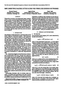
Figure 2. A snapshot of the simulation when the nodes set their connections

In Figure 2, it is shown that the nodes detect their neighbors and determine the route to sink (the user node). All nodes and the user node are stationary. The sensor network is modeled as a collection of these nodes, which transmit and receive packets over their radio channels. The channels are also modeled as specific entities, which receive messages from the nodes.

35

Figure 3. Two snapshots of the gates, first one is used for only connection but the second one is used for both connection and routing purposes.

Figure 3 shows the connection channels. A channel, which is a member of the route, is depicted at the right hand side. The other one is for an ordinary channel. Inter-layer communication within a single node is accomplished by means of message passing. When a packet is generated at a node, it is passed down from layer to layer; until it reaches the radio layer (which is called “layer0”) of the sensing node.

Figure 4. Two snapshots of the messages, first one is inter-nodal message and second one is intra-nodal message

36

In Figure 4, the packet properties are shown. A packet, which is encapsulated and to be sent from one node to the other, is depicted at the left hand side. The other one is a newborn message and has not been encapsulated yet. The radio layer generates an over the air packet, and sends it to the channel entity reserved for the routing. The channel entity than simulates the conditions of a radio channel, and delivers the packet to its neighbor, which is in the route among the nodes close enough to receive it (within the communication range). The simulation sensor model is depicted in Figure 5, below:

Figure 5. Two snapshots of the sensor nodes, first one just generated the message but second one is about to send it

37

For aggregation process, each intermediate node in the routing paths transmits a single aggregate packet even if it receives multiple input packets one after another. In other words, successive packets coming to a router node are to be aggregated and the node generates only one packet to represent all those aggregated packets. As the simulation progress, the nodes, which are under heavy traffic, begin to die one after another. The network will be accepted as alive until the time at which the user node is not satisfied with the utility level of the network any more. This time value is called the “lifetime” of the network, which is the output of the simulation for a particular parameter configuration. “After taking the definition of the utility in Chapter 2 into account, utility evaluation of this simulation is performed as follows. The user nodes expects to get all packets generated by the sensor nodes in the defined period, but it gets some of them due to some failures that have occurred on the way and due to the data aggregation used. Therefore, the utility takes a value between 0 and 1. The user is then satisfied with values that are greater than the threshold defined in Chapter 3, Problem Definition.”

Figure 6. A snapshot of the user interface of the simulation

38

In Figure 6, the output screen of the simulator is shown. Especially, in this illustration, it is understood that the user node has become isolated and therefore the simulation was stopped. The iterations are conducted until the results of all combinations are gathered. The number of iterations is: # of iterations = (# of possible values for a parameter) (# of parameters concerned) That is; 34 = 81 Moreover, for each parameter combination, we generate 10 random networks, that; The total # of iterations = 34 x 10 = 810 The next chapter, Simulation Study, interprets the results of this extensive simulation study.

39

CHAPTER 5 SIMULATION STUDY

We now present our simulation results showing the sensor network lifetime for the parameter configuration chosen. All simulations were performed in a simulation testbed in OMNeT++, a discrete event simulator environment [13], on a network of: ™

Two dimensional field of 800 x 500 cm.

™

Randomly distributed nodes on the field.

™

For each combination of the parameters, 10 simulations were run and

averaged. ™

Any runs resulting in unconnected graphs which can happen occasionally

when the values of node density and communication radius are low, were also taken into account to be able to get realistic results. The selected parameter values are again summarized in the following: B = {1000, 2000, 3000} amounts of battery capacity in mJ were used. R = {300, 400, 500} were used as communication radius in cm. T = {10, 20, 30} were taken as the query period in sec. N = {15, 30, 45} nodes scattered; one of them being the user node. In performing these simulation experiments, our goal is to understand the relations between our design parameters. In order to do that, results of many iterations were recorded on an Excel Sheet, which were then processed with a Macro

40

Program running on this excel sheet. We got 54 different unique plots as a result and 14 crucial plots of them are examined and analyzed in the following paragraphs. In the following plots, two of the parameters are fixed and the remaining two are varying. The fixed parameter values are shown at the bottom of each figure.

Figure 7. Lifetime of the Network vs. Communication Radius - 1

For the configuration seen above (i.e., query period and node density being fixed as 10 and 15, respectively), Figure 7 compares the lifetime of the network as the communication radius and initial battery capacity are varied. The figure illustrates that as the communication radius increases up to a point, the lifetime increases and beyond that point, it begins to fall. This is mainly due to the fact that

41

beyond that certain point of the communication radius, the nodes start consuming much power and this will cause them to die soon..

Figure 8. Lifetime of the Network vs. Communication Radius -2

Similar to Figure 7, Figure 8 and 9 also compare the lifetime of the network as the communication radius and the initial battery capacity are varied. The selected configurations in these plots are the node density parameter being 30 and 45 in Figures 8 and 9, respectively. It is seen from these figures that as the communication radius increases, the lifetime decreases. One thing to note in Figure 8 is the optimal value of the communication radius, which may be around 300cm for this

42

configuration. As the battery capacity increases, the margin between the lifetime values for the different communication radius becomes wider as well.

Figure 9. Lifetime of the Network vs. Communication Radius - 3

Moreover, Figure 9 illustrates a catastrophic decrease in the lifetime while the communication radius augments for this configuration. This is mainly because of the fact that in this configuration the number of nodes is high and this causes much more traffic on the network and therefore it means there will be much more power consumption per node while the communication radius increases. Hence, increasing the number of nodes in the terrain for a better coverage may lead to marginal increase after a certain point and also communication radius increases drops the life

43

considerably in such cases. The figure also shows that as the initial battery capacity increases, the lifetime increases at this ratio.

Figure 10. Lifetime of the Network vs. Query Period

For the configuration seen above (i.e., communication radius and node density fixed at 300 and 15, respectively), Figure 10 compares the lifetime of the network as the query period and the initial battery capacity are varied. It is illustrated that the increase in both the initial battery capacity and the query period causes the lifetime to increase significantly. These increases are almost linear. It is possible to conclude from this plot that there is a linear relationship between the query period and the lifetime and also between the initial battery capacity and the lifetime. This is because both of these parameters have some contribution to the network in only

44

nodal base. This means both the initial battery capacity and the query period have a direct effect on the sensor node’s lifetime. Hence, for example, if the lifetime of the nodes is increased two times then the network’s lifetime will also increase two times (i.e. by the same amount).

Figure 11. Lifetime of the Network vs. Node Density - 1

Figure 11, 12, and 13 compare the lifetime of the network as the node density and the initial battery capacity are varied. In Figure 11, the communication radius is taken as a fixed value of 300cm. It is clearly seen from this figure that when the node density goes up, the lifetime increases by decreasing amount. This is mainly due to the fact that increasing in the node density beyond a certain point causes the traffic to

45

be crowded. These figures also show that for given configuration there is a linear relation between the initial battery capacity and the lifetime.

Figure 12. Lifetime of the Network vs. Node Density – 2

For the configuration seen above (the communication radius is 400cm), Figure 12 compares the lifetime of the network as the initial battery capacity and the node density are varied. It can be seen from the figure that as if we are looking into a window showing that the lifetime is in steady state condition for this configuration given. Actually, there is an optimum value of the node density for this case. While the node density is increasing, before and after the optimum value of the node density, the lifetime is smaller than that of the optimum value.

46

Figure 13. Lifetime of the Network vs. Node Density - 3

In Figure 13, where the communication radius is 500cm, the lifetime of the network is illustrated as the initial battery capacity and the node density are varied. It is depicted in the figure that when the communication radius is 500cm, while the node density increases from 15 nodes to beyond 45 nodes, the lifetime begins to drop for this configuration given. This is because, for 500cm of communication radius, optimum value of the node density is less than 15 nodes, hence going further from that value of the node density causes the lifetime to fall slowly.

47

Figure 14. Lifetime of the Network vs. Communication Radius - 4

For the configuration seen in Figure 14, 15, and 16; it compares the lifetime of the network as the communication radius and the query period are varied. The node density is taking the value of 15, 30, and 45 nodes in Figure 14, 15, and 16, respectively. Figure 14 shows that as the communication radius increases up to a point, the lifetime increases; beyond that point the lifetime begins to fall. This is mainly due to the fact that the power consumed for transmission is related to the square of the distance and beyond a certain point of the communication radius, the nodes begins to consume much power and this will cause them to die soon. This optimum communication radius is around 400cm for this configuration chosen. It can also be seen in all those three figures that while the query period increases, the

48

lifetime goes up. This is because the scale of the lifetime of the network increases when the lifetime of a sensor node is extended.

Figure 15. Lifetime of the Network vs. Communication Radius - 5

In Figure 15, the fixed value of node density is taken as 30 nodes per area. It is illustrated in the figure that when the node density becomes 30 nodes per the area, the result in the previous scenario is different. In this case, as the communication radius increases, the lifetime begins to decrease. This is because the node density chosen is so large that one cannot find an optimum value for the communication radius by increasing it further any more. We can also extract from the figure that the optimum value for the communication radius is around 300cm

49

Figure 16. Lifetime of the Network vs. Communication Radius - 6

For the configuration seen above, the node density is 45 nodes per area, Figure 16 illustrates that when the node density become 45 nodes per the area, the result in the previous scenario is not so different. In this case, as the communication radius increases, the lifetime continues to decrease, but at this case a bit more quickly. This is because the node density chosen is too large to find an optimum value for the communication radius by increasing it further. It can be examined in the figure that, the optimum value for the communication radius is maybe around 200cm.

50

Figure 17. Lifetime of the Network vs. Communication Radius -7

For the configuration seen above, Figure 17 compares the lifetime of the network as the node density and the communication radius are varied. The selected fixed values are 3000mJ and 10 sec for the initial battery capacity and the query period, respectively. When the node density is high, it is clearly seen in the figure that as the communication radius increases, the lifetime falls rapidly. When the node density is medium, the figure shows that as the communication radius goes up, the lifetime falls gradually. When the node density is low, the figure shows that as the communication radius increases, the lifetime reaches it optimum value for the value of the communication radius, around 400cm. This is because; for all the different

51

values of the node density there is one optimal value of the communication radius. By looking the plots, we can understand somehow these values those are; for 45 nodes per the area, approximately 200cm; for 30 nodes per the area, approximately 300cm; for 15 nodes per the area, approximately 400cm.

Figure 18. Lifetime of the Network vs. Node Density - 4

For the entire configurations seen in Figure 18, 19, and 20; the figures compare the lifetime of the network as the query period and the node density are varied. It is observed from Figure 18 that as the node density goes up to a certain value, which is 45 nodes per the area here, the lifetime increases. This is mainly due to the fact that; for the constant communication radius, there is an optimum value for

52

the node density; beyond that value the lifetime begins to drop. It can also be seen in all those figures that increase in the query period causes the lifetime to increase, as stated in the pervious plots. There is one thing to note in Figure 18; as the node density goes up, the increase in the lifetime attenuates and the plot becomes almost flat.

Figure 19. Lifetime of the Network vs. Node Density - 5

Figure 19 compares the lifetime of the network as the communication radius is fixed at the value of 400 cm. The figure shows that as the node density goes up; the lifetime is almost steady for this configuration. This is mainly because of the fact that; for this value of the communication radius, the lifetime is robust against the

53

change in the number of nodes. It is depicted in the figure that increase in the query period does not change this attitude. There is one thing to note in the figure; as the node density goes up to a higher value, the increase in the lifetime become attenuate and the plot starts to fall. This is due to the fact that when the node density increases the number of massage in the network in a period will also increase and this will cause the lifetime to tend to go down.

Figure 20. Lifetime of the Network vs. Node Density - 6

As a last plot, Figure 20 represents the lifetime of the network as the query period and the node density are varied. In this case the communication radius is chosen to be 500cm. For this configuration, it is understood from the figure that as

54

the node density goes up, the lifetime begins to fall slowly. This is because; for this value of the communication radius, a node in the network consumes higher amount of energy to send a message with respect to the previous two values of the communication radius. The figure also shows that; as the node density goes up to a higher value, the decrease in the lifetime becomes larger and the plot starts to fall rapidly. This is as a result of the fact that when the node density increases, the number of massages in the network in a period will also increase and this will cause the lifetime to be attenuate.

55

CHAPTER 6 CONCLUSION

Recent advances in wireless communications and electronics have enabled the development of low-cost, low-power, multifunctional sensor nodes that are small in size and communicate in short distances. These tiny sensor nodes, which consist of sensing, data processing, and communicating components, leverage the idea of sensor networks. In some application scenarios, replenishment of power resources might be impossible. Sensor node lifetime, therefore, shows a strong dependence on battery lifetime. In a sensor network, each node plays the dual role of data originator and data router. The disfunctioning of few nodes can cause significant topological changes and might require re-routing of packets. Hence, power conservation and power management take on additional importance. It is for these reasons that researchers are currently focusing on the design of power-aware protocols and algorithms for sensor networks. In other mobile and ad hoc networks, power consumption has been an important design factor, but not the primary consideration, simply because power resources can be replaced by the user. The emphasis is more on QoS provisioning than the power efficiency. In sensor networks though, power efficiency is an important performance metric, directly influencing the network lifetime. Application specific protocols can be designed by appropriately trading off other performance metrics such as utility with power efficiency. Building self-organizing sensor networks has some challenges. All are related to map the overall system requirements down to individual device capabilities, requirements and actions. The underlying principle for building self-organizing

56

sensor networks that can overcome the challenges is to provide the fundamental mechanisms upon which other networking and system services may be spontaneously specified and reconfigured. The way sensor networks are organized internally may play a role in decreasing the energy budget to perform certain functionalities, and therefore proper design of the sensor architecture is an important goal to be pursued. To maximize the lifetime of the network, we need to minimize the energy dissipation for communication by reducing the number of sensing operations and reducing the transmission distance. There are several parameters mainly related to the network lifetime. These are initial battery capacity, communication radius, query period and node density. Since these parameters have certain trade offs in terms of the lifetime; the relations between these parameters are thoroughly investigated in this thesis. The thesis first presents a simplified system architecture for wireless sensor nodes that is capable of addressing the strict requirements of wireless sensor networks. This architecture has been applied to the developed simulation tool. We actually present a generalized architecture, which addresses the key issues that arise when building a wireless sensor network device with strict power consumption requirements. We have identified the core application scenario of environmental data collection. To validate our general architecture we have realized the following scenario: A prototype of the wireless sensor network was simulated. Simulating a suitable and application specific wireless network with the desired control parameters that are initial battery capacity, communication radius, query period, and node density was particularly difficult. Therefore, to realize the scenario as a simulation, we have made some assumptions that were defined in Problem Definition Chapter.

57

The sensor network when deployed requires itself to be able to configure and start building the network. The major goal of the deployment is to cover the maximum area within which the network will be able to function with ease. The sensor node in the network communicates efficiently with its neighbors after formation. Nodes act as both routers and sources. Due to the limited transmission range, hops are established so that the information flows from the source to the sink (i.e. user node) through the best possible way. The scenario briefly mentioned above was implemented in OMNeT++, a discrete event simulator environment. For this purpose, OMNeT++ simulation tool was installed on top of MSVC++ Version 6.0 that is already running on a NT Based Windows Operating System. In performing these simulation experiments, our goal was to understand the energy efficiency tradeoff between the sensor network parameters affecting the lifetime. Verification of the simulation was simplified by performing simulations in its animation mode, at a pace slow enough for a human expert to observe and record all simulated network behavior and compare it to that expected. The raw data is placed in a Microsoft Excel-readable file for post processing. These simulations were performed over a wide range of input parameter combinations. As a result, we got 54 different unique plots and we examined 14 crucial plots of them as illustrated in Simulation Study Chapter. In brief, four parameters were considered in this study. Two of them, initial battery capacity and query period, have directly effects on a sensor node’s lifetime. In other words, change in these parameters causes the lifetime of the network to go up linearly. In contrast, the other parameters, communication radius and node density, have trade offs in terms of the network’s lifetime.

58

We would like to note that the results of this study are somehow applicable to any kind of multihop sensor system (not only radio sensors; but also for example, underwater acoustic sensors). As a main contribution to the sensor networks, this study presents a guide to a designer. First of all, it is better for the designer to examine the whole report in order to get a feeling about the parameters of the sensor networks. After that, he/she ought to observe the results of the parameters‘selected combinations by using the analyses tool in MS Excel. After all, to be able to construct the design, the designer is supposed to execute his/her own parameter values in the simulation tool. While our specific approach is an important first step, much further research is needed in developing a detailed and accurate understanding of the interplay between the parameters considered in this study. We envision that the simulation tool designed for this analysis will play an instrumental role in the design and implementation of new application specific sensor networks. Additional exploration of network behavior as nodes fail is important. When does the network partition? How do mixes of nodes with different initial power levels affect the results? These results are likely to be sensitive to the traffic mix. Finally, experimentation is needed to validate these results with physical hardware in actual scenarios. While the platforms presented here are ready to meet the demands of realworld commercial applications, the technology enabling wireless sensor networks will continue to evolve. As advances in CMOS processes and RF radio technology are incorporated into next-generation wireless sensor nodes, the power consumption and lifetime will continually improve. The upcoming technology advances will most likely be applied to decreasing the power consumption of the device. In turn, this will enable a reduction of physical size of the energy storage required for any given application. All application

59

scenarios can benefit from reduced power consumption, which is translated into longer network lifetime. Fifteen years from now, wired sensors will be a “behind-the-scenes” technology that has grown to impact every aspect of our lives. All factory and machine command and control systems will have switched over to relying on wireless sensing and control points. The millions of miles of cumbersome wiring we hear about in building control and automation systems will be replaced by an invisible wireless mesh. The devices themselves will become as commonplace as today’s light switches and thermostats. They will be tiny, cheap, commodity pieces of silicon that interact with the physical world. Today we give little thought to modern electrical grid and what our lives would be like without it. Tomorrow we will give little thought to wireless sensor network technology and the system that have grown to impact every aspect of our lives.

60

REFERENCES

1.

C. E. Jones, K. M. Sivalingam, P. Agrawal, J. Chen, “A Survey of Energy Efficient Network Protocols for Wireless Networks”, Wireless Networks, Vol. 7, no. 4, pp. 343-358, 2001.

2.

C. Intanagonwiwat, R. Govindan, D. Estrin, “Directed Diffusion: A Scalable and Robust Communication Paradigm for Sensor Networks”, Proceedings of The Sixth Annual ACM/IEEE International Conference on Mobile Computing and Networking (Mobicom 2000) Boston, MA, pp. 56–67.

3.

D. Estrin, R. Govindan, J. Heidemann, S. Kumar, “Next Century Challenges: Scalable Coordination in Sensor Networks”, ACM Mobicom, Washingtion, USA, August 1999, pp. 263–270.

4.

C. Perkins, “Ad Hoc Networks”, Addison-Wesley, Reading, MA, 2000.

5.

S. Adlakha, S. Ganeriwal, C. Schurgers, M. Srivastava, "Density, Accuracy, Latency

and

Lifetime

Tradeoffs

in

Wireless

Sensor

Networks-

A

Multidimensional Design Perspective", Networked and Embedded Systems Lab (NESL), Electrical Engineering Department, UCLA 56-125B Eng. IV, UCLAEE Dept., Los Angeles, CA, 2003. 6.

I.F. Akyildiz, W. Su, Y. Sankarasubramaniam, E. Cayirci, “Wireless Sensor Networks: A Survey”, Computer Networks, Vol. 38, 2002, pp. 393-422.

7.

A. Woo, D. Culler, “Evaluation of Efficient Link Reliability Estimators for LowPower Wireless Networks”, Technical Report, UC Berkeley, November 2003.

61

8.

G. J. Pottie, W. J. Kaiser, “Wireless Integrated Network Sensors,” Commun. of the ACM, Vol. 43, No. 5, May 2000, pp. 51–58.

9.

K. Sohrabi, J. Gao, V. Ailawadhi, G. J. Pottie, “Protocols for Self-Organization of A Wireless Sensor Network”, IEEE Personal Communications, Vol. 7, No. 5, Oct. 2000, pp. 16-27.

10. V. Rodoplu, T. H. Meng, “Minimum Energy Mobile Wireless Networks” IEEE Journal on Selected Areas in Communications, Vol. 17, No. 8, August 1999. 11. Y. Yu, R. Govindan, D. Estrin, “Geographical and Energy Aware Routing: A Recursive Data Dissemination Protocol for Wireless Sensor Networks”, Technical Report UCLA/CSD-TR-01-0023, UCLA Computer Science Dept., May 2001. 12. B. Krishnamachari, D. Estrin, S. Wicker, “The Impact of Data Aggregation in Wireless Sensor Networks”, International Workshop on Distributed Event-Based Systems - DEBS02, July 2002. 13. OMNeT++ Home Page On The Web: http://www.omnetpp.org/

62

APPENDIX A USER MANUAL FOR THE SIMULATION AND ANALYSIS TOOL

A simulation testbed for the problem introduced in the previous chapter was implemented in OMNeT++, a discrete event simulator environment. For this purpose, OMNeT++ simulation tool was installed on top of MSVC++ Version 6.0 that is already running on an NT Based Windows Operating System. Therefore, the designer should do the following in order: ™

Install MSVC++ compiler on the operating system which can be NT, Win32

or Unix based, ™

On top of this compiler, install OMNeT++ simulation environment,

™

Copy the project and paste it into the samples directory of the OMNeT++,

™

Then the project is ready to be fetched from there by using the “Open

Workspace” command which is in the “File” menu, The parameters, which are in both “omnetpp.ini” file and “globaldef.h” file, are supposed to be adjusted according to the design. The parameters and their possible values are: ™

NNODES

{15, 30, 45};

™

NRJ_INITVAL

{1000, 2000, 3000};

63

™

INITSSTRENGTH

{300, 400, 500};

™

T

{10, 20, 30}.

Having set and saved these values in the files mentioned above, the remaining is to compile and run the project. The designer can conduct the iterations as many times as they want for a configuration chosen from the values given above. Finally, by using the results obtained, the “Macro Programmed Excel” file can be filled in. The Excel file is composed of three parts that are a result sheet, a computation module and a user interface. Here, the user interface will be introduced. In addition, the result sheet will be given in Appendix C.

Figure 21. The user interface of the Excel file

As it can be seen in Figure 21, by using the radio button, the configuration required can be obtained and in addition to the series axis, x and y-axis labels can be defined. After that, for the parameter chosen as the series axis, to be able to get all series plot, all the values of that parameter must be clicked on in order (L, M, and H).

64

Ultimately, the plot showing the relationship of the parameters with the configuration chosen will be able to be generated automatically by the macro program written.

65

APPENDIX B THE SPECIFIC SOURCE CODES

//------------------------------------------------------------------// file name: application.cpp // // - contains the implementation of application class // //------------------------------------------------------------------#include "application.h" void application::initialize() { bbaccessModule::initialize(); } void application::activity() { double Utility=1.0; int NMessageExpected =NNODES-1; int NMessageArriving=0; int sim=(int)(simTime()/10); int c=0; while(1) { if (ID!=0) // source creates messages and sends them each T seconds { UPDATECOLOR(c++); if (KIND==1) { break; } // send this message cMessage * msg = new cMessage("testmsg"); msg->setKind(M_HIGHLOW); send(msg,"lowergate_out");

66

wait(T); } else { cMessage *msga; msga = receive(); delete msga; NMessageArriving++; ev