Oriented Stochastic Data Envelopment Models: Derivation and Application ∗ Frantiˇsek Br´azdik† CERGE-EI‡ June 24, 2004

Abstract In this paper the efficiency dominance principle is used to derive oriented chance constrained models for stochastic data envelopment analysis. These models account for stochastic noise in the data used for envelopment analysis. The assumed form of error structure allows linearizing deterministic equivalents of stochastic models. To solve the linearized form of the model the interior point methods for solving linear programming problems are used. The computed efficiency scores are compared to stochastic frontier approach scores and scoring differences across used method are summarized. Keywords: stochastic data envelopment analysis, linear programming, efficiency JEL classification: C14, D24, C61

∗

This research was supported by a World Bank Fellowship. Email: [email protected] ‡ A joint workplace of the Center for Economic Research and Graduate Education, Charles University, Prague, and the Economics Institute of the Academy of Sciences of the Czech Republic. Address: CERGE-EI, P.O. Box 882, Politick´ ych vˇezˇ n˚ u 7, Prague 1, 111 21, Czech Republic †

1

1

Introduction

Data envelopment analysis (DEA) involves an alternative principle for extracting information about a population of observations, so called decision making units (DMUs), that are described by the same quantitative characteristics. This is reflected by the assumption that each DMU uses the same set of inputs to produce the same set of outputs, but the inputs are consumed and outputs are produced in varying amounts. Farrell (1957), Farrell and Fieldhouse (1962) in his seminal papers on productive efficiency stimulated research on approaches for production frontier search. DEA, developed by Charnes, Cooper and Rhodes (1978), involves an alternative approach to SFA, developed at the same time by Aigner, Lovell and Schmidt (1977), for efficiency evaluation of the population observations of decision processes. The DEA approach is a nonparametric approach to production frontier estimation and the DEA approach requires specification of the production possibility set properties instead of production function form that is required by SFA. In contrast to parametric approaches for information extraction, the objective of the DEA is to identify the smallest set that satisfies production possibility properties. Further, the estimated frontier is used to calculate the relative measure (among the elements of analyzed DMU set) of the DMU’s technical efficiency, where efficient DMUs are elements of the frontier. The general stochastic model is defined as: yj = f (xj , β)+ej , where xj represents inputs, β unknown parameters of production function f (xj , β) and yj represents output of DMUj . The composed error term ej is considered as inefficiency in DEA approach. In the SFA approach (e.g. Aigner et al. (1977), Meeeusen and van den Broeck (1977)) the error component ej is decomposed into a stochastic random component and a technical efficiency component. Therefore, together with the fact that DEA is an extreme point method the noise in data leads to mistakes in DEA efficiency scores. The dilemma of the efficiency evaluation approach choice depends on the trade off between the minimal specification that favors DEA and the handling of stochastic error in measuring DMU efficiency that favors SFA. To compete with SFA in error handling, the stochastic data envelopment analysis (SDEA) approach was developed by considering the value of inputs and outputs as random variables in the SDEA model specification. Present SDEA approaches lead to chance constrained optimization problems that consume an extensive amount of computational time for the optimal solution search even for the simple stochastic models. Random disturbances are incorporated in the SDEA model on the assumption that the probabilistic distribution of disturbances is

2

known. In this paper, two classes of efficiency dominance are defined. According to these dominance definitions the two classes of stochastic models are derived. In the process of the model development, proportional input reduction and output augmentation is introduced in the models and by use of the simplified error structure and linearization methods the linear deterministic models are derived. To solve linearized models, the interior point methods for linear programming problems are used and the large sized problems are solved with a significantly reduced amount of computational time in comparison with solving chance constrained optimization problems. The following section reviews the literature on DEA and SDEA. In the third section, notation is introduced. The fourth section defines production possibility set properties that will be used to construct stochastic models in the following sections. Two model classes will be derived according to different approaches of stochastic error inclusion. Subsequently, the model’s error structure is presented and incorporated in the model and the derivation of linearized models is described. This is followed by the introduction of the efficiency measure that is used to construct the oriented models that are linearized. The tenth section describes numerical methods that used to solve derived models. The eleventh section contributes to present development in production efficiency measurement. According to Mortimer (2002) more studies on SFA and DEA efficiency scores comparison are needed to evaluate the results consistency across different methods. I compare SDEA, DEA and SFA efficiency scores for Indonesian rice farms. The comparison reveals inconsistency between efficiency ranks acquired by SFA approach and DEA approaches.

2

Literature review

As Charnes, Cooper, Lewin and Seiford (1994) explain in their introduction, the story of data envelopment analysis begun with Edwardo Rhodes’s dissertation, which was the basis for the later published paper by Charnes et al. (1978). In his dissertation, E. Rhodes used the production efficiency concept by Farrell (1957) to analyze the educational program for disadvantaged students in the USA. Rhodes compared the performance of students from schools participating and not participating in the program. The performance was recorded in terms of inputs and outputs, e.g.:“increased self-esteem” (measured by psychological tests) as output and “time spent by mother reading with child” as input. The subsequent work on efficiency evaluation of multiple inputs and outputs technology led to Charnes et al. (1978), where the CCR model for DEA was formulated. The introduced CCR model is derived for the technology with constant returns

3

to scale. This fact is reflected in the shape of the production possibility frontier when the frontier is formed by a single ray. The efficient DMU is an element of the production possibility frontier set up by frontier ray. To handle the variable returns to scale, introduced by Farrell and Fieldhouse (1962) in to the SFA framework, the CCR model was extended by Banker, Charnes and Cooper (1984). Since the BCC model’s frontier is a piecewise linear set, Banker et al. (1984) defined weak efficiency (a weakly efficient DMU has nonzero slacks) and efficiency (an efficient DMU has zero slacks). Further, only the efficient DMUs are elements of the estimated production possibility set frontier in the framework of the BCC model. As many applications suggest, two capabilities that make DEA a powerful tool are the capability of handling multiple inputs-outputs models and that the production function form is not required. The efficiency scores in various industries are examined e.g. in air transportation Land, Lovell and Thore (1993), fishing Walden ˇ coviˇc, Halick´ and Kirkley (2000), banking Sevˇ a and Brunovsk´ y (2001), Byrnes and Valdmanis (1989) where 123 US hospitals were covered and Halme and Korhonen (1999) examines dental care units. The expanding number of papers devoted to DEA helped to identify the limitations of the DEA approach. An analyst should keep these limitations in mind when choosing whether or not to use DEA. DEA is good at estimating the “relative” efficiency of a DMU but not in “absolute” efficiency estimation. In other words, DEA reveals how well DMU is doing compared to other DMU but not compared to a “theoretical maximum.” This is the result of the analyst’s limitation in knowledge of the true production function. Figure (1) shows the difference between the true production frontier and the estimated production frontier. Since DEA is an extreme point technique, noise (even symmetrical noise with zero mean) such as measurement error can cause significant problems because the solution to optimization problems is sensitive to changes in data. As a consequence of this, theoretical attempts to incorporate these errors were made. SDEA applications are based on the theoretical paper by Land et al. (1993), where the authors used their new models to examine the efficiency of the same schooling program for disabled scholars as in Charnes et al. (1978). In Land et al. (1993), the authors offered the prospect of stochastic data envelopment analysis and constructed their own model (the LLT model). They introduced the stochastic component to DEA and derived the LLT model as a chance constrained version of BCC output oriented model in envelopment form. Further, Land et al. (1993) transformed these problems to their deterministic non-linear equivalents, which allowed them to determine the efficient DMUs.

4

Olesen and Petersen (1995) presented a different approach to incorporating the stochastic component into DEA. Olesen and Petersen (1995) assumed that the inefficiency of DMU can be decomposed into true inefficiency and disturbance term and derived the OP model from the multiplier formulation of the BCC model. The approaches of Land et al. (1993) and Olesen and Petersen (1995) to SDEA are compared by Olesen (2002) and the weaknesses of both approaches are identified. The LLT model is criticized because it does not account for all the correlations that can occur in disturbances. Olesen (2002) criticizes the OP model proposed by Olesen and Petersen (1995) because the OP model ignores correlation between DMUs and the related weakness of the OP model is omission of the fact that a convex combination of two DMUs has a lower variance than the DMUs themselves, except for the case where the input output i.d. vectors are perfectly correlated. Straightforward remedy for the OP model is to take the union of confidence regions for any linear combination of the stochastic vectors themselves rather than using a piecewise linear envelopment of the confidence regions. Olesen (2002) implemented this idea and derived the combined chance constrained model in his paper. The theoretical paper by Huang and Li (n.d.) sketches stochastic models with the possibility of variations in inputs and outputs and introduced stochastic efficiency dominance. Huang and Li (n.d.) defined the efficiency measure of a DMU via joint probabilistic comparisons of inputs and outputs with other DMUs which can be evaluated by solving a chance constrained programming problem. By utilizing the theory of chance constrained programming, deterministic equivalents are obtained for both situations of multivariate symmetric random disturbances and a single random factor in production relationships. Li (1998) obtained a linear deterministic equivalent via programming theory under the assumption of the single random factor and the stochastic supporting hyperplane is use to analyze the returns to scale. In the following sections, I will derive oriented form of models derived Li (1998) and I will use the efficiency dominance principle to obtain chance constrained equivalents to one stage oriented DEA models. The papers by Gstach (1998) and Simar (2003) show that there are research directions in which the future developments on DEA and SDEA may be driven. Gstach (1998) proposes using DEA to estimate a pseudo frontier (nonparametric shape estimation) and then apply a maximum likelihood-technique to the DEA-estimated efficiencies to estimate the scalar value by which this pseudo-frontier must be shifted downward to get the true production frontier (location estimation). Simar (2003) proposes, for cases where noise to signal ratio is low, the bootstrapping method for improving the performance of the deterministic DEA frontier estimation.

5

Mortimer (2002) in his comparative study of SFA and DEA literature summarizes the results from SFA and DEA studies to identify the amount of correlation between scores in SFA and DEA comparative studies. Mortimer (2002) calls for more studies that will compare efficiency scores correlation across production efficiency approaches. The present studies show strong correlation (e.g. Ferro–Luzzi, Ramirez, Fl¨ uckiger and Vassiliev (2003)) or very low correlation (e.g. Lan and Lin (n.d.), Wadud and White (2000)) of obtained efficiency rankings. The major problems associated with solving the DEA models are the analysis of a large set of DMUs and the solutions with zero elements. The analysis of a large data set leads to large size optimization problems that can be costly to solve. The solutions with zero elements cause problems when these solutions are interpreted as inputs and outputs shadow prices. Gonzales-Lima, Tapia and Thrall (1996) present the primaldual interior-points computational methods as the methods that significantly improve the reliability of solution in comparison to simplex methods. The interior-points methods maximize the product of the positive components among solutions, which means that the number of zero components of the optimal solution is minimized. Due to this solution’s property it is easier to interpret the DEA models results. Therefore, as the part of the theoretical work the interior point method solver is constructed.

3

Notation

In this section, the notation and definitions are introduced. The definitions will be used to construct the stochastic DEA models in the next section. The notation in this paper coincides with the notation used in Li (1998) and Huang and Li (n.d.). The task is to analyze the set of DMUj where 1 ≤ j ≤ n. Each of the DMUs is described by a random vector x ˜j , x ˜j = (˜ x1j , . . . , x ˜mj )T of m input amounts (random variables) that are used to produce s outputs in amounts described by random vector y˜j , y˜j = (˜ y1j , . . . , y˜sj )T . These vectors are aggregated to matrices of random vectors of inputs and outputs, so the following matrix notation will be used: ˜ = (˜ matrix of inputs random vectors X x1 , . . . , x ˜n ) th ˜ i row of ’input’ matrix X ˜ = (˜ xi1 , . . . , x ˜in )T , i = 1, . . . , m ix ¯ = (¯ m × n matrix of expected inputs X x1 , . . . , x ¯n ) th ¯ i row of expected ’input’ matrix X ¯ = (¯ xi1 , . . . , x ¯in )T , i = 1, . . . , m ix matrix of outputs random vectors Y˜ = (˜ y1 , . . . , y˜n ) th ˜ r row of ’output’ matrix Y ˜ = (˜ yr1 , . . . , y˜rn )T , r = 1, . . . , s rx s × n matrix of expected outputs Y¯ = (¯ y1 , . . . , y¯n ) th r row of expected ’output’ matrix Y¯ r y¯ = (¯ yr1 , . . . , y¯rn )T , r = 1, . . . , s

6

Additional notation will be introduced in the following section where the error structure is described.

4

Stochastic efficiency dominance

In contrast to the deterministic approach to envelopment analysis, DMUs are characterized by distribution moments in a stochastic approach. The production possibility set is defined by use of inputs and outputs means. Further, the second moments are used in the transformation from the chance constrained problem to its deterministic equivalent and in the approach with a chance constrained production possibility set. In this section, two classes of efficiency dominance will be defined. The first definition will be used to create almost 100% chance constrained models. The second dominance definition will be used to define chance constrained models. These models will be derived in the following sections, where the theorems that relate the efficiency dominance definition and constructed models will be mentioned. is defined as Definition 1. General stochastic production possibility set T ⊂ Rm+s + follows: T = {(˜ x, y˜) | outputs y˜ can be produced using inputs x ˜} This definition of the stochastic production possibility set relates to random vectors that characterize DMUs and it means that not all observations of DMUs are required to be an element of stochastic production possibility set. Further, the function form is not known, therefore the estimate of production possibility set is identified by the properties that the production possibility set should fulfill. Almost 100% confidence production possibility set T constructed from the set of DMUj , j = 1, . . . , n should fulfill following properties: ˜ Y˜ λ) ∈ T. Property 1. Convexity: If (˜ xj , y˜j ) ∈ T, j = 1, . . . , n and λ ∈ Rn+ , ⇒ (Xλ, Property 2. Minimum extrapolation: T is the intersection of all sets satisfying convexity and inefficiency property and subject to that each of the observed random vectors (˜ xj , y˜j ) ∈ T, j = 1, . . . , n. From these two properties follows that less output can be produced with the same inputs and this reflects the situation when some amount of inputs is wasted in the production process. The production possibility set exhibits the following property: x, y¯) ∈ T and x ≥ x ¯, then (x, y¯) ∈ T. Property 3. Inefficiency property: If (¯ If (¯ x, y¯) ∈ T and y ≤ y¯ then (¯ x, y) ∈ T.

7

˜ y˜ ≤ Y˜ λ, λ ≥ 0} satisfies the aforementioned The set T0 = {(˜ x, y˜) | x ˜ ≥ Xλ, properties. T0 is the stochastic generalization of the production possibility set of the constant returns to scale production function as used by Charnes et al. (1978) in the derivation of the CCR model. Similarly, the stochastic generalization of the ˜ production possibility set T1 for the BCC model, where T1 = {(˜ x, y˜) | x ˜ ≥ Xλ, y˜ ≤ Y˜ λ, eT λ = 1, λ ≥ 0} also satisfies the properties postulated for the stochastic production set. Later in this paper, the set T1 and its modifications will be used to derive models with variable returns to scale as in a deterministic case. Generally, the parameterized production possibility set Tϕ can be defined as fol˜ y˜ ≤ Y˜ λ, ϕ(eT λ) = ϕ, λ ≥ 0}. Tϕ includes the cases of T1 lows: Tϕ = {(˜ x, y˜) | x ˜ ≥ Xλ, and T0 for choice of parameter ϕ, ϕ ∈ {0, 1}. The concept of efficiency in DEA (based on the following relative efficiency definition) is used to define the α−stochastic efficiency dominance. Definition 2. Relative Efficiency: A DMU is to be identified as efficient on the basis of available evidence if and only if the performances of other DMUs does not show that some of its inputs or outputs can be improved without worsening some of its other inputs or outputs. The point in the production possibility set is identified as the efficient point of the production possibility set if there is no other production point that produces more output without consuming more input, or consumes less input without producing less output. This leads to the following efficiency domination definition of production possibility set element: Definition 3. Efficiency dominance: The point (x, y) is not dominated in the sense of efficiency if @ (x∗ , y ∗ ) in production possibility set such that x∗ ≤ x or y ∗ ≥ y with at least one strict inequality for input or output components. This definition demonstrates the efficiency concept of DEA and is used to derive the deterministic models, where is no possibility of a violation of the production possibility set properties or efficiency dominance. In the deterministic environment, the non-dominated elements of the production possibility set frontier set up the production envelopment surface and the Figure (1) shows the set of DMUs divided into efficient and inefficient DMUs. The efficient DMUs (represented by not dominated points) are used to set up the estimate of the production possibility frontier. The elements of the production possibility frontier estimate dominate in efficiency the other elements of the production possibility set. In the stochastic framework, the efficiency domination violations are allowed with the probability α, 0 ≤ α ≤ 1. In chance constrained programming methodology the 8

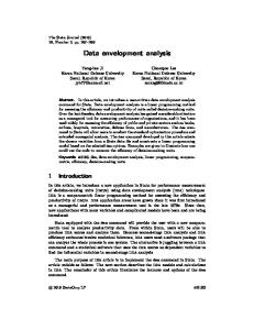
term 1 − α is interpreted as the modeler’s confidence level and α is interpreted as the modeler’s risk. The risk equals the probability measure of the extent to which specific conditions are violated. In the almost 100% confidence approach, the efficiency dominance can be violated with probability α and the production possibility constraints are almost certainly not violated. In the chance constrained model, it is allowed to violate the constraints specifying the production possibility set with probability α. For the case of the almost 100% confidence chance constrained approach, let’s consider the case where relative efficiency can be violated due to random errors and therefore the α-stochastically efficiency of point is defined as follows: x∗ , y˜∗ ) ∈ Tϕ is called Definition 4. α-stochastic efficiency of point in set Tϕ : (˜ α–stochastically efficient point associated with Tϕ ⇔ if the analyst is confident that (˜ x∗ , y˜∗ ) is efficient with probability 1 − α in the set Tϕ . This definition means that point (˜ x∗ , y˜∗ ), considered as α-stochastically efficient, is dominated (in the sense of efficiency dominance) by any other point in Tϕ with a probability less or equal to α. Using the definition of efficient point the efficiency of DMUj is defined as follows: Definition 5. α-stochastic efficiency of DMUj : DMUj is α–stochastically efficient in set Tϕ ⇔ (˜ xj , y˜j ) is point associated with DMUj and (˜ xj , y˜j ) ∈ Tϕ is an α–stochastically efficient production point in the set Tϕ . These definitions and the aforementioned properties of the set Tϕ straightforwardly imply that for efficient DMUj and for any λ such that ϕ(eT λ) = ϕ, λ ≥ 0 the expression ˜ ≤x P rob(Xλ ˜j , Y˜ λ ≥ y˜j ) ≤ α holds with at least one strict inequality in input–output constraints. To illustrate the DEA and SDEA approach, Figure (1) shows the deterministic frontier and compares it to the true production possibility frontier. The solid piecewise linear line is the unknown true production possibility frontier and the dashed line is the DEA estimate of this production possibility frontier. In Figure (2) the same DMUs are pictured and the set of α-efficiency dominant DMUs is pictured as a grey shaded area. A comparison of Figures (1) and (2) shows that the deterministic production possibility set frontier is a subset of the stochastic possibility set frontier. Due to this fact more DMUs can be identified as efficiency dominant in the stochastic framework than in the deterministic. 9

For the definition of chance constrained efficiency, the production possibility set needs to be redefined. The convexity property is replaced by confidence convexity defined as follows: Property 4. Confidence convexity: If C((˜ xj , y˜j ), α) ∈ T, j = 1, . . . , n and λ ∈ Rn+ , ˜ Y˜ λ), α) ∈ T. The confidence region C((˜ ⇒ C((Xλ, xj , y˜j ), α) is Cartesian product of input and output confidence intervals Ci ((˜ xj ), α), Cr ((˜ yj ), α) for all i = 1, . . . , m; and r = 1, . . . , s; where these confidence intervals are the smallest sets such that P rob(xi ∈ Ci ((˜ xij ), α)) = α, P rob(yr ∈ Cr ((˜ yrj ), α)) = α for i = 1, . . . , m; r = 1, . . . , s. The parameterized production possibility set that satisfies confidence convexity and minimal extrapolation property can be defined as follows:    P rob(i x ˜λ ≤ x ˜∗i ) ≥ 1 − α, i = 1, . . . , m;    ∗ ) ≥ 1 − α, r = 1, . . . , s; . TϕCC (α) = (x∗ , y ∗ ) ∈ Rm+s : P rob( y ˜ λ ≥ y ˜ r + j     T n ϕ(e λ) = ϕ, λ ∈ R , λ ≥ 0 In the almost 100% confidence approach, the production possibility set is the envelope of random vector mean values. In contrast to this, the production possibility set is a convex envelope of confidence regions that are Cartesian products of confidence intervals for means of input and output random vectors that represent observed DMUs. For the purpose of the derivation of chance constrained models, the α-chance constrained efficiency dominance and DMUj efficiency are defined in the following way: Definition 6. α-chance constrained efficiency: Point (˜ x∗ , y˜∗ ) ∈ TϕCC (α) is not dominated in the sense of chance constrained efficiency if @ (˜ x, y˜) ∈ TϕCC (α) such that P rob(˜ xi ≤ x ˜∗i ) ≥ 1 − α, for i = 1, . . . , m and P rob(˜ yr ≥ y˜r∗ ) ≥ 1 − α, for r = 1, . . . , s holds with at least one strict inequality in input or output inequalities. Definition 7. α-chance constrained efficiency of DMUj : DMUj is α-chance constrained efficient ⇔ (˜ xj , y˜j ) is point associated with DMUj and (˜ xj , y˜j ) ∈ TϕCC (α) is α-chance constrained efficient production point in TϕCC (α). In the following sections, the α-stochastic efficiency definition will be used to derive the almost 100% chance constrained problems as in Li (1998). Further, by the specifications of projection direction on the envelopment surface these models will be oriented and linearized. The same process will be applied to models according to the α-chance constrained efficiency definition and it will be shown that this definition can be used to derive the same chance constrained generalization of deterministic models as are presented in Cooper, Deng, Huang and Li (2002). 10

4.1

Stochastic model

In this section, the derivation of the almost 100% confidence chance constrained problem is reviewed. The derived model is the stochastic equivalent of the additive DEA model and will be the basis for the further theoretical development of SDEA models. In the following subsection, specific assumptions about the error structure in the data are made and the stochastic model is transformed into its deterministic equivalent. Now, from the set properties it follows that: ˜ ≤x ˜ −x {Xλ ˜j , Y˜ λ ≥ y˜j } ⊂ {eT (Xλ ˜j ) + eT (˜ yj − Y˜ λ) < 0}1 and using the probability properties the following inequality is derived: ˜ ≤x ˜ −x P rob(Xλ ˜j , Y˜ λ ≥ y˜j ) ≤ P rob(eT (Xλ ˜j ) + eT (˜ yj − Y˜ λ) < 0). Therefore, for λ such that ϕ(eT λ) = ϕ and λ ≥ 0 the condition ˜ −x P rob(eT (Xλ ˜j ) + eT (˜ yj − Y˜ λ) < 0) ≤ α is a sufficient condition for DMUj to be α–stochastically efficient. Using the sufficient condition for α–stochastic efficiency of DMUj , Cooper, Huang, Lelas, Li and Olesen (1998) constructed the following almost 100% confidence chance constrained problem (in matrix notation) for the efficiency evaluation of DMUj , j = 1, . . . , n: ˜ −x max P rob(eT (Xλ ˜j ) + eT (˜ yj − Y˜ λ) < 0) − α

(1)

λ

s.t.

P rob(i x ˜λ < x ˜ij ) ≥ 1 − ²,

i = 1, . . . , m;

P rob(r y˜λ > y˜rj ) ≥ 1 − ²,

r = 1, . . . , s;

ϕ(eT λ) = ϕ, λ ≥ 0, where ² is non–Archimedean infinitesimal quantity.2 The optimal solution of problem (1) is related to stochastic efficient point by using the following theorems: Theorem 1. Let DMUj be α-stochastically efficient. The optimal value of the objective function in the chance constrained programming problem (1) is less than or equal to zero. ˜ ≤x The inequality type change is due to the additional restriction that {Xλ ˜j , Y˜ λ ≥ y˜j } holds with at least one strict inequality. 2 This means that ² is less than any positive real number. According to chapter ”Computational P Aspects of DEA” in Charnes et al. (1994), ² < minj=1,...,n 1/ m i=1 xij is selected in the calculations of these models. 1

11

Theorem 2. If the optimal value objective functional of problem (1) is greater than zero, then DMUj in not α-stochastically efficient.3 Theorem (2) implies that if the maximum value of the chance functional ˜ −x P rob(eT (Xλ ˜j ) + eT (˜ yj − Y˜ λ) < 0) exceeds α, then DMUj is not α–stochastically efficient. The value of the chance functional of additive model represented by problem (1) can be used as the simplest efficiency measure when interpreted as the sum of input excess and output slack. In the following sections, sophisticated efficiency measures will be introduced.

4.2

Error structure

In this subsection, the error structure that allows transforming the model from a chance constrained problem to a linear deterministic equivalent is introduced and the linearization approach by Cooper et al. (1998) is summarized. The following structure of m inputs and s outputs of DMUj driven by normally distributed shocks is considered: x ˜ij = x ¯ij + aij ζij

i = 1, . . . , m;

y˜ij = y¯ij + bij ξrj ,

r = 1, . . . , s;

where it is assumed E(ζij ) = E(ξrj ) = 0, j = 1, . . . , n and following variancecovariance structure of errors for all DMUs:4 V ar(ζij ) = V ar(ξrj ) = σε2

1 ≤ i ≤ m; 1 ≤ r ≤ s; 1 ≤ j ≤ n;

Cov(ζij , ζkl ) = 0

1 ≤ i, k ≤ m; 1 ≤ j, l ≤ n;

Cov(ξrj , ξkl ) = 0

1 ≤ r, k ≤ s; 1 ≤ j, l ≤ n;

Cov(ξrj , ζil ) = 0

1 ≤ r ≤ s; 1 ≤ i ≤ m; , 1 ≤ j, l ≤ n.

Under this error structure follows: E(xij ) = x ¯ij , E(yrj ) = y¯rj and for variance 2 2 V ar(xij ) = (aij σε ) , V ar(yrj ) = (brj σε ) . When ε = ξij = ξkl = ζrj = ζil , for 1 ≤ r ≤ s; 1 ≤ i ≤ m; 1 ≤ j, l ≤ n is assumed then the assumed error structure collapses to single factor symmetric error structure where ε follows normal distribution with E(ε) = 0, V ar(ε) = σε2 . To simplify the matrix description of the shock effects to DMUs the following vector notation is introduced: 3

These theorems are corollaries of Theorem (3) in Cooper et al. (1998). For linearization procedure the standard normal distribution N (0, 1) can be assumed. The scaling of the measurement units is used when numerical problems with tiny diagonals of the input-output variance matrices occurs, therefore more generally assumption of N (0, σε2 ) is used. 4

12

aj = (a1j , . . . , amj )T , bj = (b1j , . . . , bsj )T , j = 1, . . . , n; i = 1, . . . , m, r = 1, . . . , s; i a = (ai1 , . . . , ain ), r b = (br1 , . . . , brn ), and these vectors are aggregated to construct the following matrices of input and output variations: Am×n = (a1 , . . . , an ), Bs×n = (b1 , . . . , bn ). Using the properties of normal distribution it is derived that i x ˜λ − x ˜ij is distributed 2 2 according to N (i x ¯λ− x ¯ij ; (i aλ−aij ) σε ) and (r y˜λ− y˜rj ) ∼ N (r y¯λ− y¯rj ; (brj − r bλ)2 σε2 ). Applying the inverse of cumulative distribution function Φ(α), the constraints and objective function in the almost 100% confidence chance constrained problem (1) can be rewritten and the following non-stochastic equivalent is derived: ¯ −x minλ eT (Xλ ¯j ) + eT (¯ yj − Y¯ λ)+ ¯ | σε Φ−1 (α) + | eT (Aλ − aj ) + eT (¯bj − Bλ) s.t. ¯λ ≤ x ¯ij + | i aλ − aij | σε Φ−1 (²), i = 1, . . . , m, ix −1 y¯rj ≤ r y¯λ+ | brj − r bλ | σε Φ (²), r = 1, . . . , s, T ϕ(e λ) = ϕ, λ ≥ 0.

(2)

To linearize constraints the absolute value terms from constraints in problem (2) are removed. The absolute values terms in the constraints are decomposed into the difference of two positive numbers and into the objective function the cumulative term P P ²( sr=1 (q1r + q2r ) + m i=1 (h1i + h2i )) is added. This constraint modification does not affect the optimal solutions of problem (2). Therefore, problem (2) is equivalent to the following problem with linear constraints: minλ,qkr ,hki

s.t.

¯ −x eT (Xλ ¯j ) + eT (¯ yj − Y¯ λ)+ T ¯ | σε Φ−1 (α)+ + | e (Aλ − aj ) + eT (bj − Bλ) Ps Pm +²( r=1 (q1r + q2r ) + i=1 (h1i + h2i )) ¯λ ≤ x ¯ij + (h1i + h2i )σε Φ−1 (²), ix i = 1, . . . , m, i aλ − aij = h1i − h2i , −1 y¯rj ≤ r y¯λ + (q1r + q2r )σε Φ (²), brj − r bλ = q1r − q2r , r = 1, . . . , s, T ϕ(e λ) = ϕ, λ ≥ 0, qkr ≥ 0, hki ≥ 0, k = 1, 2.

(3)

In the following step, the absolute value from the objective function is removed. The inverse of cumulative distribution function Φ(α) takes a positive or negative 13

values, to account for this factor let’s define δ such that:    −1 if α < 0.5; δ= 0 if α = 0.5;   1 if α > 0.5. The absolute value term in the objective function is the sum of the absolute value terms in constraints; therefore, the decomposition that was used in constraints is just substituted in the objective function. Thus as in Li (1998), the absolute value terms are eliminated from the objective function and the following problem with a linear objective function is obtained: minλ,qkr ,hki

s.t.

¯ −x eT (Xλ ¯j ) + eT (¯ yj − Y¯ λ)+ T −1 ¯ +δ(e (Aλ − aj ) + eT (bj − Bλ))σ ε Φ (α)+ Ps Pm +²( r=1 (q1r + q2r ) + i=1 (h1i + h2i )) ¯λ ≤ x ¯ij + (h1i + h2i )σε Φ−1 (²), ix i = 1, . . . , m, i aλ − aij = h1i − h2i , −1 y¯rj ≤ r y¯λ + (q1r + q2r )σε Φ (²), brj − r bλ = q1r − q2r , r = 1, . . . , s, T ϕ(e λ) = ϕ, λ ≥ 0, qkr ≥ 0, hki ≥ 0, k = 1, 2.

(4)

Problem (4) is known as the envelopment formulation of the DEA model, because the optimal solution identifies the projected point on to the envelopment surface for DM Uj . Now, define e as the vector of ones and as in Li (1998) the dual problem (5) to primal problem (4) is stated as follows: maxµ,ν,η,ω,ψj s.t.

µT y¯j − ν T x ¯j − η T bj − ω T aj − ϕψj µT y¯l − ν T x ¯l − η T bl − ω T al − ϕψj ≤ 0, l = 1, . . . , n; −1 −1 −1 −σε Φ (ε)µ + η ≥ −σε (Φ (ε) + ε)e − δσε Φ (α)e, −σε Φ−1 (ε)µ − η ≥ −σε (Φ−1 (ε) + ε)e + δσε Φ−1 (α)e, −σε Φ−1 (ε)ν − ω ≥ −σε (Φ−1 (ε) + ε)e − δσε Φ−1 (α)e −σε Φ−1 (ε)ν + ω ≥ −σε (Φ−1 (ε) + ε)e + δσε Φ−1 (α)e, µ ≥ e, ν ≥ e, η, ω, ψj unconstrained.

For the DMUj represented by point (˜ xj , y˜j ), the stochastic hyperplane: P rob(cT x ˜j + dT y˜j + fj ≤ 0) = 1 − ² 14

(5)

is supporting hyperplane for Tϕ at (˜ xj , y˜j ) if and only if cT x ˜j + dT y˜j + fj + Φ−1 (²)σε | cT aj + dT bj |= 0

(6)

and for ∀ (˜ x, y˜) ∈ Tϕ : cT x ˜ + dT y˜ + fj + Φ−1 (²)σε | cT aj + dT bj |≥ 0.

(7)

The derived problem (5) is known as the multiplier problem because the optimal solutions (µ∗j , νj∗ , ηj∗ , ωj∗ , ψj∗ ), j = 1, . . . , n, for the set of problems (5) set up the supporting hyperplanes used for production possibility set frontier estimation. The unique optimal solution (µ∗j , νj∗ , ηj∗ , ωj∗ , ψj∗ ) of problem (5) such that µ∗j T (bj − bk ) + νj∗ T (aj − ak ) − Φ−1 (²)σε (| µ∗j T bj − νj∗ T aj | − | µ∗j T bk − νj∗ T bk |) ≥ 0, ˜j +fj∗ ≤ 0) = 1−², for k = 1, . . . , n, identifies stochastic hyperplane P rob(µ∗j T y˜j −νj∗ T x where fj∗ = −ηj∗ T bj − ωj∗ T aj − ϕψj∗ + Φ−1 (²)σε | µ∗j T bj − νj∗ T aj |. The identified almost 100% confidence hyperplane is supporting hyperplane to Tϕ at DM Uj . In a case without an unique solution of problem (5), the supporting hyperplane for Tϕ at (˜ xj , y˜j ) is not uniquely identified. The supporting hyperplanes for the analyzed DMUs are used to construct the estimate of the production possibility frontier. Further, the sign of fj will be related to the returns to scale type in the section on returns to scale.

5

Efficiency measure

The solution of problems (4) and (5) consists of a projected point and the supporting hyperplane. The optimal solution of the envelopment problem (4) identifies the pro¯ ∗ , Y¯ λ∗ ) on the supporting hyperplane adjacent to DM Uj . jected point (ˆ xj , yˆj ) = (Xλ j j ¯ ∗ , Y¯ λ∗ ) is the optimal solution of the envelopment problem (4) and it The point (Xλ j j is an element of the hyperplane obtained as the solution of the multipliers problem (5). In this section, the projected point and envelopment defining hyperplane will be utilized to create the inefficiency measure for the DM Uj . For the purpose of a simple inefficiency measure creation, the distance measure of a discrepancy between the expected and projected point can be used. Therefore the simple inefficiency measure is (ˆ xj , yˆj ) − (¯ xj , y¯j ). This discrepancy measure expresses the difference between the efficient frontier represented by the projected point (ˆ xj , yˆj ) and the present position of DM Uj . Starting from (¯ xj , y¯j ), different projection paths on the corresponding part of the envelopment surface can be followed. Therefore various projected points and inefficiency measures can be created. The choice of projection path means the specification of the type of strategy that must to be used 15

to enhance efficiency. In the following derivation of the efficiency measure, directions of lowering inputs and increasing in outputs will be distinguished. First, for inputs of DMUj let’s denote eij ∈ R+ , eij = x ¯ij − i x ¯λ, i = 1, . . . , m and m define vector ej ∈ Rx , ej = (e1j , . . . , emj ). If P rob(i x ˜λ < x ˜ij ) > 1 − ² there must exist eij > 0, i ∈ {1, . . . , m} such that P rob(eij ≤ x ˜ij − i x ˜λ) = 1 − ². Therefore, for inputs of DM Uj , by following the path −ej the inputs can be decreased and the projected point is moved towards the production possibility frontier. This projection direction is pictured in Figure (5) as the input reduction direction. The point DMU5i is the input oriented projection of DMU#5. When the path of input reduction is used in the construction of the point projected on the production possibility frontier the input oriented DEA model is created. Similarly, the DEA output oriented model is derived using the vector of output slacks sj ∈ Rs+ , sj = (s1j , . . . , ssj ), srj = r y¯λ−¯ yrj , r = 1, . . . , s. For r ∈ {1, . . . , s} such that P rob(r y˜λ > y˜rj ) > 1 − ² exists srj > 0 for which the following equality holds; P rob(r y˜λ − y˜rj ≥ srj ) = 1 − ².5 The path sj projects DMUj on to the production possibility frontier in an outputs augmenting direction. This projection point is shown on Figure (5) as the point DMU5o. Next, to determine the maximal scale effects in inputs reduction or outputs augmentation, the projection paths sj , ej are decomposed to a proportional increase (decrease) of output (input) and residual as follows: sj = ρ¯ yj + δsj , ej = γ x ¯j + δej , where a proportional increase of outputs ρ and proportional decrease of inputs γ are defined as follows: ρ=

minr=1,...,s

γ = mini=1,...,m

yˆrj − y¯rj ≥ 0, y¯rj x ¯ij − x ˆij ≥ 0, x ¯ij

and δej ≥ 0, δsj ≥ 0, j = 1, . . . , n.6 Next as in Ali and Seiford (1993), the new variables for the output oriented model are defined as φ = 1 + ρ and for the input oriented model θ = 1 − γ. From the construction of the scaling parameters, the optimal value of θ (φ for input output problem) satisfies θ ≤ 1 (φ ≥ 1). The maximal output scale effect is identified by maximal φ and the maximal input reduction is identified by the minimal θ. For the identification of scale effects and efficiency evaluation two stage models are constructed. In the first model stage, the maximal φ or minimal θ is found 5

The same approach applies for the α-chance constrained problem. Note that at least one component of each δ is zero, because of the projection on to the production possibility frontier. 6

16

to identify the maximal proportional effect. In the second stage of modelling, the identified scale effect is utilized to optimize for envelope distance and the DMU’s efficiency is evaluated. Thus, in the first stage x ¯j is replaced with θ¯ xj in constraints and the maximal input reduction is identified by the minimal value of θ. The optimal solution to the first stage for DMUj is denoted as θˆj . Then θˆj is used in the second stage where x ¯j is replaced by θˆj x ¯j in problem (1) and the efficiency score is evaluated. Similarly, for the input oriented model y¯j is replaced by φ¯ yj and the maximal output augmentation is identified by φˆj . As in the input oriented case, the efficiency of the DMUj is evaluated by the model where y¯j is replaced by φˆj y¯j in problem (1). These two stage models are summarized in Table (2). ˆ In these models, the values of φˆ−1 j and θj can be used as the inefficiency measures. For φˆj = 1 (θˆj = 1) the point is the boundary point of Tϕ but does not necessarily represent the efficient point. The DMUj is identified as efficient if for proportional scaling parameter φˆj = 1 (θˆj = 1) and the second stage models identifies DMUj as α-stochastically efficient. The additional condition is interpreted as the sum of slacks and for α-stochastic efficiency it is required that it holds with probability 1 − α and using this condition for efficiency evaluation a class of weakly efficient points is defined. As the weakly efficient point is considered such point that fulfills only the condition on optimal value of the proportional scaling parameter φˆj = 1 (θˆj = 1).

6

Oriented SDEA models

The two stage oriented models described in Table (2) can be collapsed to one onestage model. In both stages the objective function optimization is subject to the same constraints, the only difference being the objective function. To merge these stages in one optimization problem, the non-Archimedean ² is used as a weight for the second stage objective function. The presence of non-Archimedean ² in the objective function allows such proportional movement towards the frontier that it drive out the slacks optimization. In the following sections almost 100% confidence chance constrained oriented models will be defined and their linearization will be presented. Output oriented model In this section, the almost 100% confidence chance constrained output oriented problem is linearized. The one stage model, derived from

17

the two stage optimization model presented in Table (2) is stated as follows: ˜ −x max φ + ²(P rob(eT (Xλ ˜j ) + eT (φ˜ yj − Y˜ λ) < 0) − α)

(8)

λ,φ

s.t.

P rob(i x ˜λ < x ˜ij ) ≥ 1 − ²,

i = 1, . . . , m;

P rob(r y˜λ > φ˜ yrj ) ≥ 1 − ²,

r = 1, . . . , s;

ϕ(eT λ) = ϕ; λ ≥ 0. After, the same linearization procedure, applied to problem (1) and described in the previous section, is used, and the following model is derived: ¯ −x maxλ,qkr ,hki ,φ φ − ²[eT (Xλ ¯j ) + eT (φ¯ yj − Y¯ λ)+ −1 ¯ +δ(eT (Aλ − aj ) + eT (φ¯bj − Bλ))σ ε Φ (α)]+ Pm Ps +²( r=1 (q1r + q2r ) + i=1 (h1i + h2i )) s.t. ¯λ ≤ x ¯ij + (h1i + h2i )σε Φ−1 (²), ix i = 1, . . . , m, i aλ − aij = h1i − h2i , −1 φ¯ yrj ≤ r y¯λ + (q1r + q2r )σε Φ (²), φbrj − r bλ = q1r − q2r , r = 1, . . . , s, T ϕ(e λ) = ϕ, λ ≥ 0, qkr ≥ 0, hki ≥ 0, k = 1, 2.

(9)

Input oriented model Similarly, as for the output oriented model represented by problem (8), the almost 100% confidence chance constrained input oriented model will be derived. The one stage model is created by merging the two stage optimization process presented in Table (2). The one stage model is stated as follows: ˜ − θ˜ min θ − ²(P rob(eT (Xλ xj ) + eT (˜ yj − Y˜ λ) < 0) − α)

(10)

λ,θ

s.t.

P rob(i x ˜λ < θ˜ xij ) ≥ 1 − ²,

i = 1, . . . , m;

P rob(r y˜λ > y˜rj ) ≥ 1 − ²,

r = 1, . . . , s;

ϕ(eT λ) = ϕ; λ ≥ 0. Applying the same linearization procedure as for the output oriented model the following linear deterministic equivalent of the input oriented almost 100% chance con-

18

strained model is derived: ¯ − θ¯ minλ,qkr ,hki ,θ θ + ²[eT (Xλ xj ) + eT (¯ yj − Y¯ λ)+ −1 ¯ +δ(eT (Aλ − θaj ) + eT (¯bj − Bλ))σ ε Φ (α)]+ Ps Pm +²( r=1 (q1r + q2r ) + i=1 (h1i + h2i )) s.t. ¯λ ≤ θ¯ xij + (h1i + h2i )σε Φ−1 (²), ix i = 1, . . . , m, i aλ − θaij = h1i − h2i , −1 y¯j λ ≤ r y¯ + (q1r + q2r )σε Φ (²), brj − r bλ = q1r − q2r , r = 1, . . . , s, T ϕ(e λ) = ϕ, λ ≥ 0, qkr ≥ 0, hki ≥ 0, k = 1, 2.

(11)

∗ , h∗ , φ∗ ) of problem (9) ((λ∗ , q ∗ , h∗ , θ ∗ ) for problem The optimal solution (λ∗ , qkr ki kr ki (11)) is used to evaluate the efficiency of DMUj . When the output (input) oriented model is used, the DMUj is α-stochastically efficient if the following two conditions are satisfied: 1. φ∗ = 1 (θ∗ = 1); ¯ ∗−x ¯ ∗ )|σε Φ−1 (α) ≥ 0 2. eT (Xλ ¯j ) + eT (φ∗ y¯j − Y¯ λ∗ ) + |eT (Aλ∗ − aj ) + eT (φ∗¯bj − Bλ ¯ ∗ − θ∗ x ¯ ∗ )|σε Φ−1 (α) ≥ 0). (eT (Xλ ¯j ) + eT (¯ yj − Y¯ λ∗ ) + |eT (Aλ∗ − θ∗ aj ) + eT (¯bj − Bλ As mentioned in the section on efficiency measure introduction, a class of weakly efficient DMUs can be defined. The analyzed DMUj is identified as weakly efficient when the optimal solution of the associated problem satisfies φ∗ = 1 or θ∗ = 1.

7

Chance constrained DEA model

As in the section on almost 100% chance constrained models, inputs and outputs are considered to be jointly normally distributed and the following chance constrained version of DEA model is constructed: ¯ −x min eT (Xλ ¯j ) + eT (¯ yj − Y¯ λ)

(12)

λ

s.t.

P rob(i x ˜λ < x ˜ij ) ≥ 1 − α,

i = 1, . . . , m;

P rob(r y˜λ > y˜rj ) ≥ 1 − α,

r = 1, . . . , s;

ϕ(eT λ) = ϕ λ ≥ 0; The Problem (12) is related to the definition of chance constrained efficiency domination introduced by Definition (6) by the following theorem:

19

Theorem 3. Let DMUj be an α-stochastically constrained efficient. Then for all λ such that P rob(i x ˜λ ≤ x ˜∗i ) ≥ 1 − α, P rob(r y˜λ ≥

y˜j∗ )

≥ 1 − α,

ϕ(eT λ) = ϕ, λ ∈ Rn ,

i = 1, . . . , m; r = 1, . . . , s; λ ≥ 0,

(13)

¯ −x we have eT (Xλ ¯j ) + eT (¯ yj − Y¯ λ) = 0. Proof: Suppose there exists λ∗ such that it fulfills constraints (13) and − − + ¯ ∗−x eT (Xλ ¯j ) + eT (¯ yj − Y¯ λ∗ ) > 0. Then there exists s+ r or si ∈ R+ , sr , si > 0 such − that P rob(r y˜λ∗ − y˜rj ≥ s+ xij − i x ˜λ∗ ≥ si ) ≥ 1 − α. According r ) ≥ 1 − α or P rob(˜ ˜ ∗ , Y˜ λ∗ ) which contradicts to Definition (6) the DMUj is dominated by the point (Xλ the assumption in the theorem that DMUj is α-chance constrained efficient. Applying the same orientation procedure as for almost 100% chance constrained problems the two stage problems are derived. These two stage chance constrained problems are summarized in Table (3). As for problem (1) the dual problem to problem (12) can be derived and the optimal solutions are used to identify the supporting hyperplanes to analyzed DMUs and to set up the production possibility frontier estimate. The same linearization procedure as was used to linearize problem (1) and described in previous section is applied after the two stage problem is merged in one optimization problem. The following oriented and linearized chance constrained models are derived: Output oriented model ¯ −x maxλ,qkr ,hki ,φ φ − ²(eT (Xλ ¯j ) + eT (φ¯ yj − Y¯ λ)+ Ps Pm −²( r=1 (q1r + q2r ) + i=1 (h1i + h2i )) s.t. ¯λ ≤ x ¯ij + (h1i + h2i )σε Φ−1 (α), ix i aλ − aij = h1i − h2i , y¯j λ ≤ φr y¯ + (q1r + q2r )σε Φ−1 (α), φbrj −r bλ = q1r − q2r , ϕ(eT λ) = ϕ, λ ≥ 0, qkr ≥ 0, hki ≥ 0,

20

i = 1, . . . , m, i = 1, . . . , m, r = 1, . . . , s, r = 1, . . . , s, k = 1, 2, i = 1, . . . , m, r = 1, . . . , s.

(14)

Input oriented model ¯ − θ¯ minλ,qkr ,hki ,θ θ + ²(eT (Xλ xj ) + eT (¯ yj − Y¯ λ))+ Ps Pm +²( r=1 (q1r + q2r ) + i=1 (h1i + h2i )) s.t. ¯λ ≤ θ¯ xij + (h1i + h2i )σε Φ−1 (α), ix i aλ − θaij = h1i − h2i , y¯j λ ≤r y¯ + (q1r + q2r )σε Φ−1 (α), brj −r bλ = q1r − q2r , ϕ(eT λ) = ϕ, λ ≥ 0, qkr ≥ 0, hki ≥ 0,

i = 1, . . . , m, i = 1, . . . , m, r = 1, . . . , s, r = 1, . . . , s,

(15)

k = 1, 2, i = 1, . . . , m, r = 1, . . . , s.

∗ , h∗ , φ∗ ) of Similarly, as for Problems (11) and (9), the optimal solution (λ∗ , qkr ki ∗ , h∗ , θ ∗ ) for problem (15)) can be used to evaluate the efficiency problem (14) ((λ∗ , qkr ki of DMUj as in the previous section. The DMUj is chance constrained efficient if the following two conditions are satisfied:

1. φ∗ = 1 (θ∗ = 1); ¯ ∗ −x ¯j ) = 0 and eT (φ∗ y¯j − Y¯ λ∗ ) = 0 2. All expected values of slacks are zero: eT (Xλ T ∗ ∗ T ∗ ¯ −θ x (e (Xλ ¯j ) = 0 and e (¯ yj − Y¯ λ ) = 0). To simplify the evaluation of efficiency score the following two efficiency measures for stochastic models which are stochastic equivalents for measures introduced by Tone (1993), are proposed: µ ¶ T ¯ ∗ − θ∗ x eT (Xλ ¯j ) e y¯j ∗ Input oriented: χj = θ + , T e x ¯j eT Y¯ λ∗ µ ¶ T eT (φ∗ y¯j − Y¯ λ∗ ) e x ¯j −1 ∗ Output oriented: τj = φ − . T T ¯ e y¯j e Xλ∗ The proposed efficiency measures τ and χ have following properties: 1. 0 ≤ τj , χj ≤ 1 2. χj = 1, τj = 1 ⇔ DMUj is chance constrained efficient 3. τj and χj are units invariant measures 4. τj and χj are monotonic increasing in inputs and outputs 21

5. τj and χj are decreasing in the relative values of the slacks 6. τj = φ∗ , χj = θ∗ ⇔ the expected values of all slacks are zero. These measures make it easier to evaluate the efficiency score of DMUj because they take into account the values of maximal proportional increase and the slacks (residuals) values.

8

Introducing returns to scale

Further development of the aforementioned DEA models requires the inclusion of the returns to scale type to the model specification. As it is mentioned in the section 2 the CCR model was used to analyze the set of DMUs that were using the production function with constant returns to scale. The BCC model and its variations were developed to analyze the production function with variable returns to scale. The same methodology will be used here to develop the stochastic DEA models with variable (VRS), non-increasing and non-decreasing returns to scale. To introduce the returns to scale in to the stochastic, the concept by Banker et al. (1984) is used in terms of expected values in the following definition: Definition 8. Returns to scale. Let DMUj be stochastically efficient and the point Zδ = ((1 + δ)¯ xj , (1 + δ)¯ yj ) is point in δ–neighborhood of (¯ xj , y¯j ) : • The Non-Decreasing returns to scale are present ⇔ ∃ δ ∗ > 0 such that Zδ ∈ Tϕ for δ ∗ > δ ≥ 0 and Zδ ∈ \ Tϕ for − δ ∗ < δ < 0 • The Constant returns to scale are present ⇔ ∃ δ ∗ > 0 such that Zδ ∈ Tϕ for | δ |< δ ∗ • The Non-Increasing returns to scale are present ⇔ ∃ δ ∗ > 0 such that Zδ ∈ \ Tϕ ∗ ∗ for δ > δ ≥ 0 and Zδ ∈ Tϕ for − δ < δ < 0. The various types of returns to scale are reflected by different shapes of the production possibility set frontier that is set up by the intersection of supporting hyperplanes identified by solutions of multiplier problems. In the case of constant returns to scale (the CCR model by Charnes et al. (1978)) the envelopment surface consists of a single half line that passes through origin as it is shown in Figure (3). Figure (3) also presents the production possibility frontier of the model with the variable returns to scale that is referred to as the BCC model. In the case of VRS presence the frontier is a piecewise linear set. These types of returns to scale of 22

production possibility set are parameterized via the selection of ϕ and constraint type associated with the ϕ as follows: ( 0 Constant returns to scale (CCR model) ϕ= 1 Variable returns to scale (BCC model). Since the α-stochastically efficient point (˜ xj , y˜j ) satisfies condition (6), for the point Zδ = ((1 + δ)¯ xj , (1 + δ)¯ yj ) can be derived: cT (1 + δ)˜ xj + dT (1 + δ)˜ yj + fj + (1 + δ)Φ−1 (²)σε | cT aj + dT bj | = = (1 + δ)(cT x ˜j + dT y˜j + fj + Φ−1 (²)σε | cT aj + dT bj |) − δfj = −δfj .

(16)

Therefore the point Zδ ∈ Tϕ if and only if −δfj ≥ 0. Employing definition (8) the relation between returns to scale and the sign of fj is revealed. The returns to scale type is reflected in the type of the constraint ϕ(eT λ) = ϕ for ϕ = 1. The Table (1) summarizes the constraint variations and relates the constraint type on λ, the returns to scale type and frontier hyperplane characteristic.

9

Summary of SDEA models

In the previous sections the various models were derived and related to definitions of α-stochastic and chance constrained efficiency dominance. Table (4), which summarizes these models, is presented. It is evident that the models based on a different efficiency dominance definition lead to different evaluation of efficiency scores. It should be stressed that even the models using the same efficiency dominance definition but with different orientation choice lead to different results. Therefore, the choice of the efficiency dominance type, returns to scale and projection path to the envelopment surface (the set of dominating points in the production possibility set) is a crucial choice for the efficiency analysis. The important choice for efficiency score evaluation is the choice of the efficiency measure. The returns to scale choice affects the shape of the production possibility set envelopment. The restrictions on returns to scale are related to four types of the envelopment surface shape through the geometry of the production possibility set and these restrictions are interpreted as the restriction on λ in the envelopment problem or a restriction on supporting hyperplanes in the multiplier problem. The evaluation of efficiency score is based on distance measurement between the point that represents DMU and the associated point on the envelopment surface. This distance measure used in additive models is the most simple efficiency measure.

23

A more sophisticated efficiency measure is created using the measure of maximal proportional inputs reduction (output augmentation) while keeping the levels of outputs (inputs) fixed. This proportional input (output) scaling approach is interpreted as the selection of a projection path towards the envelopment surface and results in the creation of oriented SDEA models. The use of Non-Archimedean infinitesimal ² is closely related to unit invariance property of the objective function values of the derived models, because the result of multiplication by ² is not unit dependent and its role is to distinguish between the efficient and inefficient DMUs, which are elements of the production possibility set boundary. The use of unit invariant models also delivers the possibility of units of measurement change when numerical problems (e.g., tiny diagonal matrices) are expected to arise when the models are solved. In Table (4), the presented SDEA are compared only with the most popular DEA models that appear in the present literature. The additional SDEA models can be created as the extensions of models covered in this paper using the extensions procedures for DEA models.

10

Method for SDEA model solving

To solve the linear problems associated with SDEA models the interior point method (IPM) is used. IPM is used because it is less computationally costly than the simplex methods for large sized problems. The second reason for IPM use is that the IPM solutions satisfy the strong complementarity slackness condition (SCSC). The SCSC solution is the solution with the maximal product of the positive components of the optimal solution. Therefore, SCSC solutions are optimal solutions with a minimal number of zero components.7 In the case of a not unique optimal solution, the SCSC solution is not the vertex of the optimal solution set as it is in the case when the simplex algorithm is used. Simplex type algorithm searches for the optimal solution among the vertices of the feasibility set, therefore the optimal solution is a vertex (vertices). The IPM generates the infinite sequence of points that converges to an optimal solution and the iteration process stops when the iterations are sufficiently close to the optimal solution. For the purpose of IPM use the linearized problems can be easily transformed to 7

For more details on the use of interior point methods solutions of DEA related problems see Br´ azdik (2001).

24

the standard linear programming form: Primal:

min cT x s.t. Ax = b, x ≥ 0

Dual:

max bT y s.t. AT y + z = c, z ≥ 0.

(17)

In the case of linearized stochastic problems, vectors x, c, z ∈ Rn+3(m+s)+1 ; vectors y, b ∈ R2(m+s)+1 and matrix A ∈ R(2(m+s)+1)×(n+3(m+s)+1) . When using the primaldual version of interior point method the primal and dual problem (17) is solved simultaneously. The optimal solution of the linear programming problem associated with the DEA model consists of envelopment and multiplier problem solutions and these solutions are utilized to evaluate the efficiency of the analyzed DMU and the identification of the adjacent supporting hyperplane. Using the complementarity constraint zT x = 0 (equivalent to duality gap condition cT x − bT y = 0) together with the feasibility constraints the following optimality condition for problem (17) is stated:     0 Ax − b     T (18)  A y + z − c  =  0 , T 0 z x where z, x ≥ 0. The strict complementarity solution to problem (18) is such solution (x, z, y) that xi +zi > 0, ∀i = 1, . . . , n+3(m+s)+1. In the case that the problem (18) solution set is not a singleton set (the problem (17) does not have unique solution) the set of strict complementarity solutions is equal to the set of SCSC solutions. In the case of a unique solution to problem (17), the unique solution to problem (18) is the SCSC solution. To solve problem (18) usually a variant of Newton’s method is used. The created solver uses the Mehrotra’s predictor-corrector algorithm that belongs to the class of path following IPM algorithms. The algorithm uses the combination of Newton’s direction (gap decreasing direction) and centering direction to solve the sequence of problem (18), where the complementarity constraint is modified to xTk zk = µk and sequence µk converges to 0 for k → ∞. The iteration process stops if the problem is solved with the desired accuracy or the limit for the number of iterations is reached. The solver for the proposed SDEA models is constructed using the procedures package known as PCx linear solver obtained from Optimization Technology Center at Argonne National Laboratory and Northwestern University.

25

11

Indonesian rice farms efficiency

In this section the SDEA model efficiency ranking is compared with SFA and DEA (for separate periods) model efficiency ranks. Indonesia is the biggest rice importer in Asia at the same time almost 70% of the country’s 213 million people are farmers. The identification of the linkages between different factors and rice yield in West Java area is subject of many studies on farming efficiency ( e.g. Druska and Horrace (2004), Wadud (2002) and Daryanto, Battese and Fleming (2002)). The used data set was previously examined by Druska and Horrace (2004)8 , where the authors examined spatial effects on efficiency ranking s and I will use SFA ranking by Druska and Horrace (2004) as a benchmark for SDEA and DEA rankings. For research purposes Indonesian Ministry of Agriculture surveyed 171 rice farms over six growing periods (3 wet and 3 dry periods) in six villages in area of Cimanuk River basin in West Java. The used data set is a selection from this survey. The data on Indonesian rice farms are in the form of a balanced panel for 171 farms in six periods. I will show that for this data the approach to efficiency evaluation matters, because efficiency rankings are not consistent across used methods. To eliminate misreported and excessive data, the data set is filtered for outliers according to their yield per hectare performance by 1% data cut off from above, so the balanced panel still contains farms with a wide range of per hectare yields. The stochastic envelope is estimated in 5 inputs and 1 output space. The considered inputs include total area of rice cultivation in hectares (ha), seed in kilograms (kgs), urea in kilograms (kgn), phosphate in kilograms (kgp) and total labor (lab). As the output the total output of rough rice in kilograms (grkg) is considered. The data, aggregated across farms, are summarized in Table (5). The piecewise Cobb-Douglas production possibility frontier is assumed, therefore the data were transformed by taking logs before efficiency evaluation. All of the production factors exhibit very high variation and it is expected that these variation values have an influence on efficiency evaluation. The high variation in data gives a rationale for the use of the SDEA approach and I will also compare the deterministic DEA efficiency rankings with the SDEA rankings. To estimate the efficiency scores the one stage output linearized model with constant returns to scale in the form of Problem (14) with ϕ = 0 was used. The estimated results do not exhibit high variance in scores with respect to changes in modeler’s risk, therefore only results for α = 0.05 are reported. 8

For more references on Indonesian rice farm studies see the reference section in Druska and Horrace (2004).

26

The idea is to see how the efficiency scores and rankings differ across the standard DEA, SFA and SDEA models. The efficiency scores summary statistics are in Table (6). The table reports higher mean values of efficiency scores for data envelopment approaches. Table (7) compares efficiency scores for DMUs that were chosen according to the SFA efficiency score by Druska and Horrace (2004) to represent farms with the highest, median and the lowest technical efficiency. Large differences in efficiency scores are observed. To take closer look at efficiency distribution, Figure (6) displays the kernel density estimates of efficiency scores and reveals the peaks in distributions of efficiency scores. These peaks can be caused by differences in approaches because the SFA approach allows only one DMU to achieve a score of 1 but in data envelopment approaches this is score is assigned to all DMUs on the production possibility frontier. This explains the high peak in density function for SDEA efficiency score for values close to 1. The high variation in data can be the cause for the large number of efficient DMUs in SDEA because the number of DMUs identified as efficient is increasing with respect to the size of modeler’s risk and the size of variance coefficients. Therefore, rather than efficiency scores the ranks in efficiency scoring are compared. Table (8) compares the ranks of selected DMUs and large differences are also observed for selected farms. To compare estimated efficiency ranks, the Spearman rank correlation coefficient and significance for the test of the hypothesis that considered rank series are not correlated. The Spearman correlation coefficient is used because its important feature is lower sensitivity to extreme values in comparison to correlation of standard Pearson correlation coefficient. Low coefficient values are observed and most of the correlation coefficient estimates are not significantly different from zero. This comparison contrasts with the study by Ferro–Luzzi et al. (2003), where the SFA and DEA methods were used to evaluate the efficiency of regional employment offices. Ferro–Luzzi et al. (2003) reports significant correlation coefficients between SFA and DEA ranking in range from 0.594 to 0.677. Here, the highest significant estimate of rank correlation coefficient 0.2583 between SFA and data envelopment approach is observed for DEA efficiency scores in the fourth period.

12

Conclusions

The contribution of this theoretical paper is the development of four oriented stochastic DEA models and a description of their properties. Also, the α-chance constrained efficiency dominance is defined and it is shown that the efficiency dominance ap-

27

proach leads the chance constrained generalization of deterministic DEA models for mean values of input and output characteristics. Using the techniques of stochastic problems linearization the proposed stochastic models were linearized, so the interior point methods for linear problems can be used to solve linear programming problems associated with the models. The created solver for problems associated with the SDEA models, uses primaldual interior point method algorithm and both primal and dual solution are utilized in efficiency evaluation and estimation of production possibility frontier. The derived models were applied to evaluate the efficiency scores of Indonesian rice farms. I conclude that the estimates of efficiency scores and ranks depend on the methods used because I was not able to deny the hypothesis that the ranks are independent across the methods. The data envelopment approach results in scores with higher variance than the stochastic frontier approach. These findings above are consistent with the recent comparable studies, e.g. Wadud and White (2000) and Jaforullah and Premachandra (2003). The further research on farming efficiency will focus on identification of spatial effects in rankings and search for factors that can improve farms’ efficiency scores. Acknowledgment I am grateful to Viliam Druska for data and SFA efficiency scores from study on Indonesian rice farms by Druska and Horrace (2004). Also, I would like to thank Michal Kejak for his supervision during World Bank Fellowship programme and Jan Kmenta for useful comments.

References Aigner, Dennis, C. A. Knox Lovell, and Peter Schmidt, “Formulation and estimation of stochastic frontier production function models,” Journal of Econometrics, July 1977, 6 (1), 21–37. Ali, Agha Iqbal and Lawrence M. Seiford, The measurement of productive efficiency: Techniques and Applications, New York: Oxford University Press, Banker, R. D., Abraham Charnes, and William W. Cooper, “Some Models for Estimating Technical and Scale Inefficiencies in Data Envelopment Analysis,” Management Science, 1984, 30, 1078–192. Br´ azdik, Frantiˇ sek, “Interior point methods in DEA models of linear programming,” master thesis, Faculty of mathematics, physics and informatics of Comenius University, Mlynsk´a dolina, Bratislava, Slovakia June 2001. in Slovak. 28

Byrnes, Patricia and Vivian Valdmanis, Cost Analysis Applications Of Economics and Operation Research, Berlin: Springer Verlag, 1989. Charnes, Abraham, William W. Cooper, and E. Rhodes, “Measuring the efficiency of decision making units.,” European Journal of Operational Research, 1978, 2, 429–444. , , Arie Y. Lewin, and Lawrence M. Seiford, Data Envelopment Analysis: Theory, Methodology and Applications, Kluwer Academic Publishers, 1994. Cooper, William W., Honghui Deng, Zhimin Huang, and Susan X. Li, “Chance constrained programming approaches to congestion in stochastic data envelopment analysis,” February 2002. unpublished. , Zhimin Huang, Vedran Lelas, Susan X. Li, and Ole B. Olesen, “Chance Constrained Programming Formulations for Stochastic Characterizations of Efficiency and Dominance in DEA,” Journal of Productivity Analysis, 1998, 9, 53–79. Daryanto, Heny, George E. Battese, and Euan M. Fleming, “Technical Efficiencies of Rice Farmers Under Different Irrigation Systems and Cropping Seasons in West Java.” PhD dissertation, University of New England, School of Economics, University of New England, Armidale, NSW, Australia July 2002. Asia Conference on Efficiency and Productivity Growth. Druska, Viliam and William C. Horrace, “Generalized Moments Estimation for Spatial Panel Data: Indonesian Rice Farming,” American Journal of Agricultural Economics, 2004, 86 (1), 185–190. Farrell, M. J., “The Measurement of Productive Efficiency,” Journal of the Royal Statistical Society. Series A (General), 1957, 120 (3), 253–290. and M. Fieldhouse, “Estimating Efficient Production Functions under Increasing Returns to Scale,” Journal of the Royal Statistical Society. Series A (General), 1962, 125 (2), 252–267. Ferro–Luzzi, Giovanni, Jos´ e Ramirez, Yves Fl¨ uckiger, and Anatole Vassiliev, “Performance measurement of efficiency of regional employment offices,” National Research Project 45, Universit´e de Gen´eve, D´epartement d´economie politique 40, Boulevard du Pont-dArve CH-1211 Gen´eve 4 October 2003. 29

Gonzales-Lima, Maria D., Richard A. Tapia, and Robert M. Thrall, “On the construction of strong complementarity slackness solutions for DEA linear programming problems using a primal–dual interior–point method,” Annals of Operations Research, 1996, 66, 139–162. Gstach, Dieter, “Another approach to data envelopment analysis in noisy environments: DEA+,” Journal of Productivity Analysis, 1998, 9, 161–176. Halme, Merja and Pekka Korhonen, “Restricting Weights In Value Efficiency Analysis,” October 1999. Huang, Zhimin and Susan X. Li, “Chance Constrained Programming And Stochastic Dea Models.” School of Business, Adelphi University, Garden City, New York. Jaforullah, Mohammad and Erandi Premachandra, “Sensitivity of technical efficiency estimates to estimation approaches: An investigation using New Zealand dairy industry data,” University of Otago Economics Discussion Papers 0306, University of Otago, Department of Economics, University of Otago, P.O. Box 56, Dunedin, New Zealand October 2003. Lan, Lawrence W. and Erwin T.J. Lin, “Measuring Technical and Scale Efficiency in Rail Industry: A Comparison of 85 Railways Using DEA and SFA,” Traffic and Transportation, 21, 75–88. Land, K.C., C.A.K Lovell, and S. Thore, “Chance-constrained Data Envelopment Analysis,” Managerial and Decision Economics, 1993, 14, 541–554. Li, Susan X., “Stochastic models and variable returns to scales in data envelopment analysis,” European Journal of Operational Research, 1998, 104, 532–548. Meeeusen, W. and J. van den Broeck, “Efficiency estimation from Cobb-Douglas production Functions with Composed Error,” International Economic Review, 1977, 18, 435–444. Mortimer, Duncan, “Competing Methods for Efficiency Measurement: A Systematic Review of Direct DEA vs SFA/DFA Comparisons,” Working paper 136, Centre for Health Program Evaluation, Centre for Health Program Evaluation, P.O. Box 477, West Heidelberg Vic 3081, Australia September 2002. Olesen, O. B., “Comparing and Combining Two Approaches for Chance Constrained DEA,” Technical Report, The University of Southern Denmark December 2002. 30

Olesen, O.B. and N.C. Petersen, “Chance constrained efficiency evaluation,” Management Science, 1995, 41, 442–457. Simar, L´ eopold, “How to Improve the Performances of DEA/FDH Estimators in the Presence of Noise,” Technical Report 0328, Institut de Statistique Universit´e Catholique de Louvain, Belgium August 2003. Tone, Kaoru, “An Epsilon-Free DEA and a New Measure of Efficiency.,” Journal Of The Operations Research Society Of Japan, 1993, 36 (3), 167–174. ˇ coviˇ Sevˇ c, Daniel, Margar´ eta Halick´ a, and Pavol Brunovsk´ y, “DEA analysis for a large structured bank branch network,” Central European Journal of Operations Research, 2001, 9 (4), 329–343. Wadud, Abdul, “A comparison of Methods for Efficiency Measurement for Farms in Bangladesh,” July 2002. Asia Conference on Efficiency and Productivity Growth. and Ben White, “Farm household efficiency in Bangladesh: a comparison of stochastic frontier and DEA methods,” Applied Economics, October 2000, 32 (13), 1665 – 1673. Walden, John B. and James E. Kirkley, “Measuring Technical Efficiency and Capacity in Fisheries by Data Envelopment Analysis Using the General Algebraic Modelling System (GAMS): A Workbook,” report, National Marine Fisheries Service, Woods Hole, Massachusetts October 2000.

31

A

Figures and Tables Output

Frontiers

4

Production frontier

DMU3 3 DMU2

Estimated Production frontier

DMU5 2 DMU4

DMU1 Efficient

DMUs DMU1 1 DMU4 Ineffiecnt

DMUs

Input 1

2

3

4

5

6

Figure 1: DEA estimate of production possibility frontier

32

Output

Stochastic Frontier

4

DMU3

Estimated Production frontier

3 DMU2 DMU5 2

DMU1

Efficient DMUs

DMU5

Ineffiecnt DMUs

DMU4 DMU1 1

Input 1

2

3

4

5

6

Figure 2: Set of α-stochastic dominant points

Output

Frontier Shape

4

DMU3

Constant RTS

3 DMU2 DMU5 2

Non- Increasing RTS

DMU4 DMU1 1

DMU1

DMU

Input 1

2

3

4

5

6

Figure 3: Returns to scale - Constant, Non-Increasing

33

Output

Frontier Shape

4

DMU3

Non- Decreasing RTS

3

DMU5 2

BCC Model

DMU2 DMU4

1

DMU1

DMU DMU1 Input 1

2

3

4

5

6

Figure 4: Returns to scale - Non-Decreasing, BCC model

Output

Projection Orientation

4

DMU3

DMU5o

3

Productin Frontier

DMU2 Output Augmentation DMU1

2

DMU

DMU5i

DMU1

DMU5 Input Reduction

1 Projected Points

Input 1

2

3

4

5

6

Figure 5: Projection on the production possibility frontier

34

SFA SDEA DEA average

0

2

Density 4

6

8

Density estimate

.2

.4 .6 Efficiency score

.8

1

Figure 6: Kernel density estimates

Model (Orientation) CCR model (Input, Output)

Returns to scale

Constraint

Hyperplane(s)

Constant

None, ϕ = 0

Passes trough origin

BCC model (Input, Output)

Variable

eT λ = 1

Not constrained

SDEA models (Input) (Input) (Input) (Output) (Output) (Output)

Non-Decreasing Non-Increasing Constant Non-Decreasing Non-Increasing Constant

eT λ ≥ 1 eT λ ≤ 1 None eT λ ≥ 1 eT λ ≤ 1 None

Table 1: Returns to scale

35

fj∗ fj∗ fj∗ fj∗ fj∗ fj∗

≥0 ≤0 =0 ≤0 ≥0 =0

36

P rob(r y˜λ > y˜rj ) ≥ 1 − ² ϕ(eT λ) = ϕ λ≥0 i = 1, . . . , m; r = 1, . . . , s.

Second stage ˜ − θˆj x maxλ P rob(eT (Xλ ˜j ) + eT (˜ yj − Y˜ λ)) − α s.t. P rob(i x ˜λ < θˆj x ˜ij ) ≥ 1 − ²

Second stage ˜ −x maxλ P rob(eT (Xλ ˜j ) + eT (φˆj y˜j − Y˜ λ)) − α s.t. P rob(i x ˜λ < x ˜ij ) ≥ 1 − ² P rob(r y˜λ > φˆj y˜rj ) ≥ 1 − ² ϕ(eT λ) = ϕ λ≥0 i = 1, . . . , m; r = 1, . . . , s.

Table 2: Two stages of oriented almost 100% confidence chance constrained models

minλ,θ θ s.t. P rob(i x ˜λ < θj x ˜ij ) ≥ 1 − ² P rob(r y˜λ > y˜rj ) ≥ 1 − ² ϕ(eT λ) = ϕ λ≥0

Input oriented model First stage

maxλ,φ φ s.t. P rob(i x ˜λ < x ˜ij ) ≥ 1 − ² P rob(r y˜λ > φ˜ yrj ) ≥ 1 − ² T ϕ(e λ) = ϕ λ≥0

Output oriented model First stage

37

P rob(r y˜λ > y˜rj ) ≥ 1 − α ϕ(eT λ) = ϕ λ≥0 i = 1, . . . , m; r = 1, . . . , s.

Second stage ˜ − θˆj x maxλ eT (Xλ ˜j ) + eT (˜ yj − Y˜ λ) s.t. P rob(i x ˜λ < θˆj x ˜ij ) ≥ 1 − α

Second stage ˜ −x maxλ eT (Xλ ˜j ) + eT (φˆj y˜j − Y˜ λ) s.t. P rob(i x ˜λ < x ˜ij ) ≥ 1 − α P rob(r y˜λ > φˆj y˜rj ) ≥ 1 − α ϕ(eT λ) = ϕ λ≥0 i = 1, . . . , m; r = 1, . . . , s.

Table 3: Two stages chance constrained models

minλ,θ θ s.t. P rob(i x ˜λ < θj x ˜ij ) ≥ 1 − α P rob(r y˜λ > y˜rj ) ≥ 1 − α ϕ(eT λ) = ϕ λ≥0

Input oriented model First stage

maxλ,φ φ s.t. P rob(i x ˜λ < x ˜ij ) ≥ 1 − α P rob(r y˜λ > φ˜ yrj ) ≥ 1 − α T ϕ(e λ) = ϕ λ≥0

Output oriented model First stage

38

Variable Variable Constant Constant

BCC BCC CCR CCR

Variable Constant

Variable Constant

Almost 100% confidence oriented models, Problems (11),(9) (input, output)

Chance constrained oriented models Problems (15),(14) (input, output)

(input) (output) (input) (output)

Constant Variable

Almost 100% confidence additive model; Problem (4)

model model model model

Returns to Scale Variable Constant

Model (Orientation) Additive

linear linear linear linear

0 < θ ≤ 1, 1 ≤ φ 0 < θ ≤ 1, 1 ≤ φ

0 < θ ≤ 1, 1 ≤ φ 0 < θ ≤ 1, 1 ≤ φ

0