Motion Capture System on an FPGA 6.111 Final Project Report
Lauren Gresko Elliott Williams December 11, 2013
1
Table of Contents Overview 3 Design Overview 419 1. Video System 49 1.a Motion Detection 1.b Serial Interface 1.c 3D Mapping 2. 3d Graphics System 919 Design Process and Experience 2028 Testing 29 Results 30 Conclusion 37 Acknowledgements 37 References 37 Appendix 38 A: System Block Diagram B: Video System B1: Video System Sender B1.a Detection Module B1.b Center of Mass Module B1.c Cross Hair Module B1.d Clock Divider B2: Video System Receiver B2.a Recieve data B2.b Match B2.c Match bones C: 3D Graphics System
2
Overview Motion capture, or recording and animating an object or person, is a commonly researched technology with a variety of applications. Motion capture is often employed in the fields of computer animation, video games, films, music, medicine, sports, robotics, and defense. For our final project, we designed and attempted to implement our own ‘mocap’ system that would capture a user's movements and animate them on the monitor. While the image capture was implemented successfully, time and hardware constraints prevented the graphics system from being realized. Theoretically, our mocap system would have captured position data accurately and displayed a simple animation in realtime. This simplified mocap system offers a robust solution to a commonly studied problem of replicating human motion. Our mocap system covers the basics of motion capture, while also offering the challenge of implementing a complex system on the 6.111 lab kit. To create a 3D motion capture system, we used two cameras that face the user at 90 degree angles from each other. Using either colored sweat bands, we track the user’s joints and generate a list of 3D coordinates that are used to reconstruct a skeletal model of the user. We will then attempted to use this model to generate a 3D model of the user’s movements on a computer screen. In the final product, the user were able to move around their arms, and observe as there joint coordinates were tracked. With an additional week or so of work, the 3D graphics system could have been completed, allowing the used to view a 3D image on the monitor mimicking their motions. In our minimal design we tracked a user's forearms. This required the tracking of four separate points. The generated 3D model would have been a simple collection of rectangular prisms to represent the user's arms. Further iteration of this design could be improved to include the tracking all of the user's body parts, for a total of eleven points (if we are clever, it might not be necessary to track 11 colors (an impossible task)).
3
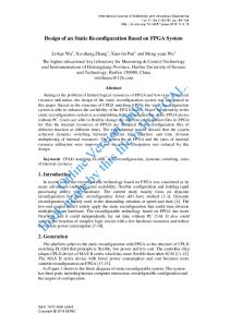
Design Overview This document describes the proposed design of our motion capture system. The project is partitioned into two sections: the video system module and the graphics system module. The video system processes the video received from our two cameras into a usable format for our 3D graphics system. The 3D graphics system creates a 3D model based on the information it received from the video system. Figure 1 depicts the overall block diagram of our motion capture system.
Figure 1: The Overall Block Diagram for the Motion Capture System. Above is a block diagram of the various modules that comprise the motion capture system. The Motion Capture System is composed of two blocks, the Video System (containing the Motion Detection and 3D Mapping subsystems) and the #D Graphics System (containing the 3D Model Generator and the Frame Rendering subsystems). The arrows represent the inputs and outputs of the modules. Additionally, the clock will connect to all of the blocks in the system; however for simplicity, the clock arrow connections have not been displayed.
1. Video System (Lauren) The video system captures the location of the user's joints, generating a 3D skeleton to be displayed by the 3D graphics system. As shown in Figure 1, the functionality of the video system depends on two main modules, the motion detection module and the 3D mapping module. The motion detection system tracks the colors sources on the user, therefore tracking the points and movement of the user’s arms. The 3D mapping module processes the resulting position data to determine the (x,y,z) skeletal coordinates of the user. 4
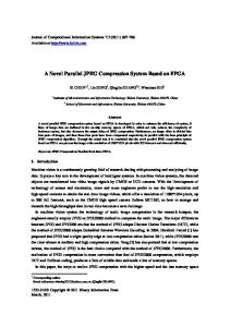
Figure 2 depicts the submodules of the Motion Detection and the 3D mapping modules, as well as introduces a new module: the Serial FPGA Interface. As shown in Figure 2, The Video System incorporates two cameras which are each wired to their own FPGA. To combine the data from each camera, a serial interface was created to transfer data from one FPGA to the other. As depicted in Figure 2, one FPGA has a sender module, while the other FPGA has a receiver module. Once the receiver FPGA receives the (y,z) coordinates from the sender FPGA, the 3D Coordinate generator maps the (x,z, color) bits with the (y,z,color) bits based on color. The submodules of the Motion Detection, Serial FPGA Interface, and 3D Mapping modules are described in the following section.
Figure 2: The Block Diagram for the Video System. Above is a block diagram of the various modules that comprise the video system. The video system is composed of five main processing modules and two modules for interfacing the two FPGAs used. Green blocks are located on the first FPGA, i.e. the sender, while blue blocks are used to depict modules on the second FPGA, i.e. the receiver. The (x4) or (x2) depicts how many instances of each module were used. The arrows represent the inputs and outputs of the modules. Additionally, the clock will connect to all of the blocks in the system; however for simplicity, the clock arrow connections have not been displayed.
a. Motion Detection Module 5
The motion detection module decodes the video signals from both cameras to generate (x,z) and (y,z) coordinates for each of the four different color sources. As depicted in Figure 3, the user wears four different color sources (terry cloth bands) at four different points on their body: the right wrist, right elbow, left wrist, and left elbow. The module first detects the pixels that match the hue, saturation, and value limits (hsv values) that correspond with each color. It then performs a center of mass calculation on these pixels to determine the coordinates of the color source's center. This process is completed twice, once for each camera, to get both the (x,z) and (y,z) coordinate pairs.
Figure 3: User input: four color sources. This diagram shows the four color sources (blue, yellow, red, and green) that the user of the motion capture system will be wearing, as viewed from the two camera inputs to the system. By placing color sources on the user’s wrists and elbows, the motion detection module tracks the endpoints of the user's forearm and upper arm in two coordinate planes (x,z) and (y,z).
The motion detection module is made up of four sub modules, the Video Decoder, RGB to HSV, Point Detection, and the Center of Mass Detection sub modules. The following section contains the details and processes for each of the sub modules. All of these modules were designed by Lauren. These sub modules, along with the rest of the system's sub modules, are depicted in Figure 4 in the appendix. Video Decoder: 6
The video decoder converts the NTSC and Ycrcb input video data to RGB video data. This step is necessary to allow further conversion into HSV video data. This module is provided by the 6.111 staff, and has been modified to output color video in RGB rather than the black and white. This module is used twice; it will be used on the (x, z) video data and the (y, z) video data. Input: clock, video camera stream Output: RGB bit stream RGB to HSV: The RGB to HSV converts video data using the RGB color space protocol into video data using the HSV color space protocol. This conversion is important because the HSV color space provides more space between color values, making subsequent point detection easier. This module is used twice; it will be used on the (x, z) video data and the (y, z) video data. This module is also provided by the 6.111 staff. Inputs: clock, RGB bit stream Outputs: HSV bit stream Point detection: This module takes the HSV stream of bits and detects which pixels correspond to the color source, accumulating the correct color locations to enable the center of mass detection module to determine the location of each color source. This detection is done by comparing the hue, saturation, and value of the HSV bit stream to the color sources that the user would be wearing. In this project, this module is instantiated 4 times; and parameters (the hue_min, hue_max, sat_min, and val_min) determine which of the 4 colors the instance is looking to match and therefore which of the 4 points (R wrist, R elbow, L wrist, L elbow). This module is used twice; it is used on the (x, z) video data and the (y, z) video data. Parameter: hue_min, hue_max, sat_min, and val_min Inputs: clock, HSV bit stream Outputs: matched pixels Center of Mass Detection: This module determines the center of mass of the user’s arm joints. This center of mass determines the coordinate location of each color source in the (x,y) and (y,z) planes. This does the by averaging the position of all the matching pixels. Then, in addition, every four pixels are averaged in center_mass module. This module is used twice to calculate both (x, z, color) and (y, z, color) coordinates. Inputs: clock, matched pixels Outputs: (x, z, color) or (y, z, color) which represent the coordinates of the designated body part (the L wrist, L elbow, R wrist, or R elbow).
c. Serial Interface Module As shown in Figure 2, The Video System incorporates two cameras which are each wired to their own FPGA. To combine the data from each camera, a serial interface was created to transfer data from one FPGA to the other. A frame_pulse signal is generated every new frame, i.e. when hcount and vcount are equal to zero, while the 7
interface_clock was created by dividing the 40hz system clock by an 8 bit counter. The two FPGAs are then linked by six wires that are connected via the user1[0:5] I/O pins on each FPGA. Pin 1 is connected to interface_clock, pin 2 is connected to the frame_pulse, and pin 0, pin 3, and pin 4 are connected to yellow_data, green_data, and blue data respectively. As depicted in Figure 2, this serial interface is comprised of a sender module and a receiver module, that processes these various signals. Sender: A 2D coordinate and its color index are sent every frame (i.e. on every frame_pulse). This data is sent serially, i.e. one bit of the coordinate at every positive clock edge. Instead of sending the full hsv or rgb value across the wire, the sender sends a color_index, which is a 2 bit number corresponding to one of the four colors. In the implemented scheme, the color_index for red, yellow, green, and blue are 0, 1, 2, and 3 respectively. Inputs: (y,z, color) Outputs: data, frame_pulse, clock_interface Receiver: Once the slowed down interface_clock, the frame pulse, and the data have reached the receiver FPGA, the receiver module reconstructs the data sent using a 24 shift register that is then split into y,z, and the color index. Inputs: clock_interface, frame_pulse, data Outputs: (y,z,color_index)
c. 3D Mapping Module The 3D mapping module merges the coordinate data generated by the motion detection module into a group of 3D coordinate pairs that comprises the user's joints. The 3D mapping module first maps the (x,z) and (y,z) coordinates of the four color sources together based on the color. The module then matches the (x,y,z) points of the right wrist to the (x,y,z) of the right elbow, and the (x,y,z) points of the left wrist to those of the left elbow. This matching results in a forearm “bone” that would have been passed to the graphics module to generate a realtime 3D model of the user’s arms. The 3D mapping module is made up of two sub modules, the 3D Coordinate Generator and the Skeleton Generator. The following section contains the details and processes for each of the sub modules. All of these modules are designed by Lauren. These sub modules, along with the rest of the system's sub modules, are depicted in Figure 4 in the appendix. 3D coordinate Generator: This module creates the 3dimensional (x,y,z) coordinates of each point from the (x,z, color) and (y,z, color) coordinates, thus detecting the locations of all of the user's joints. This module handles hidden points, i.e. when a color source is hidden from one or both of the cameras, by setting the xyz coordinate to the previous xyz coordinate if one of the coordinates have gone to zero (has not been detected). Input: clock, (x , z , color) and (y, z, color) coordinates 8
Output: (x,y,z, color) coordinates Skeleton Generator: This module matches the (x,y,z, color) coordinates of the left wrist with the left elbow and right wrist with the right elbow. These matched coordinates would have been outputted as “bones” to be drawn, providing the 3D graphics system with a 3D skeleton of the user's location. Input: clock, (x,y,z) coordinates Output: matched elbow and wrist (x, y, z), (x,y,z) coordinates
2. 3D Graphics System (Elliott) The 3D graphics system generates and displays a 3D model of the user based on the 3D skeleton generated by the video system. As shown in Figure 1, the graphics system is also divided into two parts, the 3D Model Generator and the Frame Rendering module. The 3D Model Generator uses the skeleton generated by the video system to create a 3D model of the user when viewed from a predetermined viewpoint. The frame renderer draws this model to the display. Each of these systems are composed of submodules built on mathematics wrapper modules. These modules provide the abstraction necessary to design around the large number of signal wires necessary; a single coordinate being composed of four, eighteenbit, fixed point numbers, resulting in seventy two wires per coordinate. The use of fractional math is necessary to produce the necessary shading and transform effects. Note that the Python prototype is well commented and uses the exact same algorithms (or slightly modified versions) as the hardware modules described below. Therefore, the python code in Appendix C is highly recommended as a guide to better understand the algorithms described below.
a. Model Generator Module The 3D model generation module creates and manages a 3D model of the viewer. Figure 4 below provides a helpful illustration of the process this module used by comparing the stages of the 3D graphics with the production of an image using a camera. First the object that is to be viewed is created. Then the camera is placed to view the object from a specified angle. Next the camera takes the picture, capturing the object in its viewing volume and creating the effect of perspective. Finally, the negative is prepared so that the object is centered in the photograph.
9
Figure 4: An illustration of the model generation process. This diagram compares the model generation process with the process of creating a photograph. The camera is first positioned to capture the object in a specific location and orientation. Then the image is captured, creating perspective. Finally the image is centered on the photograph. [2]
The Model Generator module is made up a state machine that manages the inputs and outputs of its five different sub modules to perform the graphics operations described above. These the Prism Generator, the Shader, the Vector Normalizer, and the View, Projection, and Viewport Transformer submodules. Each of these submodules are composed of matrix math wrapper modules which are themselves composed of fixed point math wrapper modules. The Prism Generator module creates the rectangular prism from the bone coordinates. The View Transformer alters the coordinates of this prism to view it from a specified angle and orientation. Next the Projection Transformer adjusts the coordinates further to create the perspective effect. This transformation disrupts the homogeneous nature of the coordinates (discussed in detail in the transformer module descriptions below). Therefore, the coordinates are normalized by the Vector Normalizer module to restore the homogeneous property. Finally, the View Port Transformer shifts the coordinates to be screen pixel coordinates, allowing the 10
Renderer to draw the image. To provide a greater sense of depth, the sides of the prism are shaded to create the illusion that the prism is lit by a simple uniform light source. This functionality is created by the Shader module using the side normal vectors generated by the Prism Generator. The following section contains the details and processes for each of the Model Generator’s sub modules. All of these modules were designed by Elliott. The main submodules of this system are depicted in Figure 5 below.
Figure 5: An overview block diagram of the Model Generator module. This module calculates the coordinates and colors of the image to be displayed on the screen by the Rendering module.
Rectangular Prism Generator: This module generates a set of eight vertexes (x,y,z) that compose a rectangular prism centered around each provided “bone” and the corresponding normal vectors for each side. These prisms represent the user's arm segments and are the objects on which the rest of the 3D graphics system will operate on.
Figure 6: The vertex coordinate system chosen to generate the model and shade colors.
11
To create the vertex points and normal vectors, the Prism Generator first calculates the bone vector by subtracting one point from the other. It then normalizes this vector to create the unit bone vector which is the unit normal vector perpendicular to the front and back of the cube as shown in figure 6 above. The cross product of this vector and the unit x vector (1,0,0) is then calculated, creating an arbitrary vector perpendicular to the bone vector. This vector is then normalized to create the unit normal vector, Unit Perp A, of the top and bottom faces (the faces are illustrated in figure 6 ). The cross product of the unit bone vector and Unit Perp A is then taken, generating the Unit Perp B vector perpendicular to the left and right faces in figure 6. Note that the cross product of two unit vectors is itself a unit vector. The resulting unit normal vectors are then scaled by the prism width and added to the supplied points to produce the eight vertices that define the rectangular prism. For example, P1 in figure 6 is generated by adding Unit Perp B and Unit Perp A to P1. Note that if the result of the initial cross product is ( 0, 0, 0), then the unit bone is parallel to the x axis and the two necessary perpendicular vectors (Unit Perp A and Unit Perp B ) can be arbitrarily chosen to be the unit y and unit z coordinates. The hardware inplemetation of this modules is a massive pipeline that updates the inputs of the math submodules whenever all of the outputs all ready. This pipeline allows for the maximum throughput with minimum resources, though a slower state machine implementation could have been used to consume less resources. Input: clock, matched elbow and wrist (x, y, z), (x,y,z) coordinates Output: the eight vertexes (x,y,z) of a rectangular prism in standard coordinates View Transformer:
This module performs the matrix multiplication necessary to transform standard coordinates based around the origin into coordinates based around the camera's point of view. This transformation includes three rotation transformations around the x, y, and z axis before a translocation transformation that shifts everything to the right coordinates. This is accomplished by using four matrix multipliers in a row with the proper transform matrix shown in figure 7 below. Note that this module has a propagation delay of four clock cycles, once for each transform, yet has a throughput of one. Because each matrix multiplier uses up 16 multipliers, the size of this module could have been greatly reduced by using only one matrix multiplier and changing the input matrix. This would have been a slower module, yet this would go unnoticed because the View Transformer is not the system’s bottleneck.
12
Figure 7: The translocation and x,y,z rotation matrices used to calculate the view transform. [2]
Input: clock the eight vertexes (x,y,z) of a rectangular prism in standard coordinates Output: the eight transformed vertexes (x,y,z) of a rectangular prism Projection Transformer: This module performs the matrix multiplication necessary to transform view coordinates into projection coordinates that account for perspective. This transformation includes a single matrix multiplication. The effect of this transformation is to stretch the
coordinates by proportions of the viewing frustum depicted in figure 8 below. Objects closer to the view take up proportionally more space in the viewing frustum and thus appear larger than distant objects. This creates the effect of perspective. This transformation is accomplished by using the transform matrix shown in figure NUMBER below.
Figure 8: The view frustum that defines the projection transform. [2]
13
Figure 9: The transform matrix for the projection transform. [1]
Input: clock, the eight vertexes (x,y,z) of a rectangular prism in camera coordinates Output: the eight transformed vertexes (x,y,z) of a rectangular prism Normalizer:
This module normalizes the coordinates of a homogeneous vector by dividing all of its components by W. This restores the homogeneous property and allows further transformations to be performed. This is module is implemented as a buffer that feeds a divider with the proper inputs one at a time. Input: clock, a scaled homogeneous vector Output: the normalized homogeneous Viewport Transformer: This module performs the matrix multiplication necessary to transform projection coordinates into pixel coordinates to be drawn to the screen. This transformation includes a single matrix multiplication. The effect of this transformation is to shift the center of the coordinate system to be at the center of the screen and to scale the coordinates so that the maximum and minimum world coordinate values appear at the edges of the screen. Depending on the coordinate inputs from the Motion Capture system this module might be used twice, once to map the input coordinates to center around the origin for the graphics transformations and once to shift the coordinates back to pixel coordinates. However, the necessity of a second copy of this module was not ascertained because the graphics system was not completed. Note that this module (in addition to the other transform modules) utilizes homogeneous coordinates. These coordinates are simply normal ( x, y, z) 14
coordinates with an additional one term (w) appended at the end. The w term enables a four by four matrix to transform the coordinates in many different ways that are not easily performed in nonhomogenous coordinates. This transformation is accomplished by using the following matrix. Note that dt is the x coordinate scale factor, dy is the y coordinate scale factor, dv is the z coordinate scale factor, and that dx, dy, dz are the x, y, and z coordinate shift factors. [ dt, 0, 0, dx ] [ 0, du, 0, dy ] [ 0, 0, dv, dz ] [ 0, 0, 0, 1 ] Input: clock, the eight vertexes (x,y,z) of a rectangular prism in projection coordinates Output: the eight transformed vertexes (x,y,z) of a rectangular prism in pixel coordinates
Shader:
This module calculates the appropriate ambient and directed light incident on each face of the rectangular prism. This light scale factor is proportional to the magnitude and amount of light reflected by the face and inversely proportional to the square of the distance from the light source to the face. The value is calculated by first taking the dot product of the face’s normal vector and the unit light vector. This dot product is equal to the magnitude of the two vectors multiplied by the cosine of the angle between them. Because both vectors are unit vectors, the magnitudes are 1, making the dot product equal to the cosine of the angle between them. This function provides the perfect scale factor based on the angle; the scale factor is 0 when the light and face are parallel (and this no light is reflected) and 1 when the light and face are perpendicular (and all of the light is reflected). The dot product is then multiplied by a fixed scale factor before being dividing by the square of the distance from the light source. To keep the module simple, the light source was chosen to be a uniform light source originating from the z = 0 plane and pointing in the positive z direction. This means that the distance between the light sources and the object is just the z coordinate of the object. Again to make the module simpler, the z coordinate of each face was fixed at average value of its vertices z coordinates. A more complicated shading algorithm would have colored each pixel separately based on its distance from the light source. An ambient light factor is then added to ensure that faces parallel to the light source were not completely black (an unrealistic result). Finally the scale factor is clamped to lie between 0 and 1. This shading creates a much greater sense of depth in the final image. 15
Input: clock, the six unit normal vectors of the rectangular prism's six faces Output: the shading factor of the rectangular prism's six faces
b. Renderer Module The Rendering module takes the 2D coordinate values and shaded color values and displays a properly scaled 2D image on the VGA screen. This is accomplished by using ZBT memory to store image data that could be read by a VGA module and written to by a pixel drawing algorithm. The original plan was to have the module use a double frame buffer in ZBT memory so that it could update one frame while displaying another. This buffer would have enabled real time graphics if the rest of the system was fact enough. This plan was made infeasible by the needs of the system and the limitations of both hardware and time. This infeasibility is discussed in the Design Process and Experiences section below. Therefore, instead of using a double frame buffer to create a dynamic image, the Renderer was scaled down to be a single frame buffer that creates a static image. Data is first cleared from the buffer, then drawn to the buffer, and then finally read from the buffer. This simplified control system is not ideal and was used purely to demonstrate that the Renderer system worked. The Renderer module is divided into five sub modules, the Polygon Drawer, the Memory Converter, the Pixel Buffer, the Memory Control, and the ZBT to VGA modules. The data into and out of the ZBT memory is controlled by the Memory Control module. The Pixel Buffer controls the input to the memory by mediating between the Polygon Drawer and the Memory Controller. Finally the VGA module controls the output signals. Ina complete final design, the state of the renderer would have been tightly controlled by a toplevel state machine that better managed when the buffer would be cleared, written to, and drawn from. The following section contains the details and processes for each of the sub modules. These sub modules, are depicted in Figure 9 below in the appendix.
Figure 9: An overview block diagram of the Renderer module. This module takes in
16
coordinates and colors and generates an image on the screen.
Polygon Drawer: This module draws and calculates the z value for each pixel contained within the polygon described by the four input points. The module works by first calculating the plane equation parameters ( A, B, C ,D in A*x + B*y + C*z = D) by using the Calc Plane Equations sub module. Then the algorithm calculates the bounds of the draw space by finding the minimum and maximum x and y coordinates set by the vertices. Next the algorithm calculates the slope and x intercept for each of the sides of the polygon using the slope line equation: x = M*y + B. M is calculated from the equation M = (x2x1)/(y2y1). B is then calculated from B = x2 – M*y2. Finally it uses a divider to invert C, allowing the depth of each pixel to be calculated using only dividers and multipliers and the equation z = (A*x + B*y D)*C^1. This concludes the precalculation section of the algorithm. For each y value between the minimum and maximum y values, the algorithm follows the following procedure. First the x value of the intersection between each of the sides that intersect the y coordinate and the y coordinate is calculated from x = M*y + B. Because the polygons are guaranteed to be simple, there will only be two intersections. These values are then sorted to find the beginning and end x values for that specific y pixel. The algorithm then iterates over every x value between these endpoints, calculates the depth from the above equation, and draws the pixel. This repeats until y reaches y max. This hardware implementation of this algorithm is a state machine that goes through the several initialization calculation states before iterating between the intersect calculation and pixel drawing states until the polygon is shaded. Input: clock, the four vertexes (x,y,z) of a rectangular prism in pixel coordinates Output: location, z_write, color Memory Converter: This module converts the x, y, and z data from the Polygon Drawer and the shaded color value into the corresponding memory address and data to be written to ZBT. Filters the Pixel ready signal from the Polygon Drawer to ensure that only pixels within the screens bounds are drawn to the screen. The data packing method is one leading zero followed by a two bit color index to select between green, red, blue, and yellow, followed by a 4 bit shade value supplied by the Shader module, followed by the eleven bit depth value calculated by the Polygon Drawer. The address is simply the y location followed by the top 8 bits of the x index. A selector bit is used to determine if the pixel is in the first or second half of the word in the specified memory location. Input: clock, read location, color, z read, Output: write location, z_write, color_write, z_read, read location, color_read
17
Pixel Buffer: This module mediates between the Memory Controller and the polygon drawer. The buffer simply supplies the memory control with a constant stream of pixels to write because the Polygon Drawer has a higher throughput but provides the pixels in spurts. This constant stream maximizes the system’s throughput because the Memory Control module is the system’s bottleneck. This module also lets the Memory Controller know when a pixel is available and disables the Polygon Drawer when the buffer is full. This way, neither the Pixel Drawer or the Memory Control modules have to worry about how the timing of the other works. This simplifies the toplevel Renderer module control because the Pixel buffer takes complete control of the data flow. Input: clock, read location, color, z read, Output: write location, z_write, color_write, z_read, read location, color_read Memory Controller: This module manages the state of the memory buffer. It is a simple state machine that clears the memory, then writes the data, and then switches into read mode permanently. It also manages what signals are written and read from the ZBT. In the clear state, the ZBT’s write enable is set high and the input is fixed so that the color values are all set to black and the depth is reset to a high value. Then after at least one vsync and a debug switch is enabled, the state switches into the write state. In the write state, the ZBT is alternatively read from and written to. The ZBT is read from in order to compare the depth values, though this depth functionality was not implemented in time. This module then writes back the read value, replacing the proper pixel value with the pixel read from the pixel buffer. Once the drawer is finished, this module permanently enters read mode (unless a debug switch is flipped). It is important to note that this module is rudimentary and was design to debug other modules and was being constantly modified at the last minute for other debugging purposes. The next step in my design would be to redesign this module to be better thoughtout and written. Input: clock, read location, color, z read, Output: write location, z_write, color_write, z_read, read location, color_read ZBT to VGA: This module manages the generation of the proper signals to control the VGA monitor.It communicates with the frame buffer module to read and display the proper pixel values. The implementation is a modified version of the the example code provided by the 6.111 staff. The modification changed the module to read from memory every other pixel instead of every four pixels. It also changed what data was read from memory for each pixel and implemented a look up table to read color values from. Output: read location, display_addr, VGA control signals 18
c. Matrix Math Wrapper Modules To perform all of the operations necessary for the top level modules and submodules described above, several matrix math wrapper functions were necessary. They are as follows:
Pack Matrix: This module packs 16 input wires into a four by four matrix Unpack Matrix: This module unpacks 16 output wires from a four by four input matrix Pack Vector: This module packs 4 input wires into a homogeneous vector Unpack Vector: This module unpacks 4 output wires from a homogeneous vector Matrix Multiplier: This module Multiplies a 4 by 1 input vector by a 4 by 4 input matrix, returning a 4 by 1 output vector. Vector Sum: This module returns the sum of two input vectors, ignoring the w components Vector Dif: This module returns the difference of two input vectors, ignoring the w components Vector Scale: This module multiplies an input vectors by a scalar, ignoring the w components Dot Product: This module takes the dot product of two input vectors, ignoring the w components Cross Product: This module returns the cross product of two input vectors, ignoring the w components and setting the resultant output vectors w value to one
Coord Normalizer: The module divides each element in a vector by w. Has a Tpd of 32 cycles and a throughput of 0.25 Vector Divider: The module divides each element in a vector by an input scalar. Has a Tpd of 32 cycles and a throughput of 0.25 19
Magniture: The module calculates the magnitude of an input vector. Has a Tpd of 9 cycles and a throughput of 1/9. Matrix Inverse: The module finds the inverse of an input vector. Noninvertible case is ignored because it is rare in the context this module is used in. Calc Plane Equation: This module calculates the plane equation parameters for the plane containing three input points. Based on the following derivation. Plane equation: Ax+By+Cz = D note that D is arbitrary because it simply scales A,B,C Q = [A,B,C]^T M = [v1,v2,v3] > M*Q = D > Q = M^1 * D Note: Z = (Ax+ByD)/C
d. Fixed Point Math Wrapper Modules To ensure accuracy of transformations, fixed point fractional numbers had to be used. However, Verilog does not contain fixed point objects, therefore, wrappers had to be created to perform the necessary calculations. The wrapper modules are as follows: Pack:
Packs an integer and a fractional component into a fixed point number Unpack:
Unpacks the integer and fractional components of a fixed point number Mult:
Multiplies two fixed point numbers. Note that the decimal place is doubled by the multiplication so the result must be right shifted. Also ensure that result stays within the bounds of the min and max product Divides:
Dividess two fixed point numbers. Note that the decimal place is halved by the division so the result must be left shifted. Also ensure that result stays within the 20
bounds of the min and max quotient Sqrt:
Calculates the square root of a fixed point number. Note that the decimal place is halved by the root function so the result must be left shifted. Unlike the divider module, the sqrt model does not provide a fractional remained, making the square root only accurate up to PS/2. Module is based on module supplied in the lecture slides. Sine:
Implements a simple look up table to find the sine of a fixed point number. Note that this function would only be needed to change the viewing angle and thus does not need to be very precise. Cos:
Implements a simple look up table to find the cos of a fixed point number. Note that this function would only be needed to change the viewing angle and thus does not need to be very precise.
21
22
Design Process and Experiences Video System Design Process and Experience (Lauren) This section outlines the design choices for the Video system, as well as highlights sections of the project that were most difficult. For the design process, the Video system was built off of the zbt sample module provided by the 6.111 staff. I edited the module to output color, i.e. RGB, then I used a staff module to convert RGB into HSV. Once I had that working, I was able to begin color detection based off of HSV values. First, I started with one color (red) and tried to distinguish it from the background by hue alone. I overlayed the video feed with red pixels where red was being detected. I soon found that hue min and max values were not enough to differentiate between colors; the ranges of hue for yellow and red were far too similar. I then incorporated saturation and value limits (SV of HSV) so that I was using all 18 bits of HSV to decode where colors were located. I found ranges of hsv by making the hue_max, hue_min, sat_min, and val_min limits adjustable by buttons 0 through 3 on the lab kit, and displaying the current values on the hex display. As I adjusted the range, I could see how much red the camera detected within the current limit. I used the adjustable limits to find values for red, then red but not yellow, then yellow but not red, then green, and then finally blue. Differentiating between red and yellow was very difficult, because their hue is so similar, but yellow has a much higher saturation minimum. By making the saturation value higher for yellow, and the saturation value of yellow much lower than that of red’s, I was able to differentiate between the colors. Moreover, looking at the HSV spectrum for red, the red hue wraps around the possible ranges, i.e. the red range includes both the maximum hue values as well as the minimum values, but not the values in between. To compensate for this, red detection included high values or low hue values, while yellow detection focused on low values alone. Once yellow and red were detected, I incorporated green, which was actually the easiest color to detect. Then finally, I worked on incorporating blue. Blue was the most difficult color to track, and it did not help that then entire 6.111 lab is blue. At first, our blue arm band was too dark to track. The camera was unable to detect any color pixel in the dark blue arm band, because not enough color was reflecting. In order to find a replacement blue, I ordered another variety of colors of armbands off Amazon. Looking at the hsv space, I suspected that purple would be a good replacement 23
blue, because purple falls in a large range of HSV values. It turned out that blueishpurple worked well, and I was finally able to detect all four colors. Another difficulty with color detection was that colors look different at different angles and in different lighting. Using my adjustable HSV limits, I was able to fine tune my values so that the color of the arm band was able to be detected from all the angles the arm band would be used from. Additionally, I found that the camera detects better if it is above the user, i.e. angled downward. This is due to the location of the light source on the color arm band; the lights in lab are all located on the ceiling. At times I used an additional desk lamp to shine on my arm bands, however pointing a desk lamp directly at the user caused the luminosity of yellow to become too bright. Next, I developed a center of mass module that each frame, goes through and increments a count for every color pixel determined between the hue, sat, and val limits of a specific color, and adds the x and y (actually the z coordinate based off of our model axes) coordinates to an x accumulator and a y accumulator. Using Coregen, I created dividers to average the accumulator by the count of pixels. This implementation caused the center of mass detection to still be a tad glitchy, so I added in the four pixel average module I had used to display HSV values on the hex display. This module creates a running average, by storing the most recent coordinates in an array, adding up the four coordinates, then dividing the sum by four, i.e. shifting by two. This module helped to smooth the glitchiness of the center of mass detection. Next, I made a serial interface module to merge the data being collect from the first camera, with that of the data being collected by the second camera. To transmit the coordinates of each of the color sources, I wired up six user I/O pins from the sender FPGA to the receiver FPGA. One wire was used for each color (4 wires total), one wire sent across the slowed down interface_clock, and one wire sent across a ‘frame pulse.’ This frame pulse was created every time a new frame began, and signaled to the receiver that the sender was about to start sending bits. Because I was sending data serially across long wires, I slowed down the system clock to avoid noise from the parasitic resistance of the wires. I divider the system clock of 40mhz by an 8 bit clock, and used this interface_clock to serially send 24 bits per frame (2 bits of color index, 11 bits of x coordinate, and 10 bits of y coordinate). I used a color index, 2 bits of data corresponding to a specific color (red=0, yellow=1, green=2, blue=3), rather than sending the entire HSV value to reduce data flow. On the receiving end, I created a receiver module that reconstructs the serially sent data 24
into three different registers: the color index, the x coordinate, and the y coordinate. On the receiving end, I noticed my data signal was shifted by one clock cycle, i.e. it always sent one zero before sending my actual data, which in turn shifted all of my data by one. I fixed this issue by collecting data for an extra time cycle and throwing away the first value I collected. Finally, I created the 3D mapping section. I output the x,z and the y,z on the hex display trying to figure out how to determine the final z. Conveniently, there was not much of an offset between the two z’s, so I chose to use the z from the second camera because it seemed slightly more stable than that of the z from the front view. Because I had sent the colored yz values across separately (x_new_r and y_new_r) and I had detected the colored xz seperately (x_red and y_red), I was able to match 3D coordinates solely based on their color. One difficult aspect of the 3D mapping was hidden points. My detection module outputs a center of mass or a zero, based on whether or not enough pixels were detected. I decided to handle hidden points by defining them to be when not enough pixels were detected, i.e. an output of zero. Whenever a coordinate was detected to be zero, I set the coordinate to be the value of the last known coordinate, then output the xyz with that data. One issue with this implementation is the similarity between red an yellow. Depending on the angle the colored arm band was viewed from, yellow could appear to have some red pixels and vice versa. As a result, the detection may calculate the center of mass of the incorrect arm band, as opposed to realizing it is a hidden coordinate. The successful detection of a hidden coordinate is also dependent on objects in the background, for example, if the blue lab bench is in view of the screen, the detection may not realize there is a hidden point if the minimum count of points is satisfied. Further work on this project would include improving the hidden point detection to take these factors into consideration. Once I had these x,y,z, color_index pairings, I was able to combine these pairings into the bone pairings. For creating bones, I combine two x,y,z,color_index pairings (a wrist and an elbow) into a 66 bit bone. When I made my instances of the match_bones module, I decided to create it such that it always pairs red and green while always pairing yellow and blue. Because this matching is hard coded, the user must always wear red and green on one arm, while wearing yellow and blue on the other. The 66 bit bones were then ready to be sent to Elliott via another serial interface, using the same scheme described above. As discussed about, the most difficult part of the project was finding good HSV values that would work for all four color sources. In addition, debugging the video 25
system was at times very tedious. Because the calculations depended on input from the cameras, behavioral simulations were not helpful. A large amount of time was spent recompiling changes to see how it affected the functionality. Moreover, various timing and placement issues arose due to the size of the project. Each detect module had four dividers, and there were four detect modules on each FPGA. When ISE placed the design, it at times would not optimize paths that were crucial to correct functionality of the system. As a result, more time was spent recompiling to try to open a working bit file, then this bit file was saved for later use. For example, because we were not interfacing the two halves of the project together, I wanted to display my 3D bone coordinates on the display, and use a switch to flip between the two arms. This was working great, until the last couple days of the project, when after one compile time, the hex display stopped working entirely. I had saved the bit file, so I was able to show the 3D point functionality, however, it was very frustrating that I could not use the 3D point hex display in the final days of the project. If the hex display did begin to work, it was often at the cost of the video display not working, which was not work having the hex display operate correctly. Moreover, as discussed above hidden points were a big challenge and are not always perfect when yellow in a certain light is also red. Overall, the Video system was a challenging system to integrate, and I learned a lot about using an FPGA in a large scale project. Although we were unable to combine our projects in the end, the work we both did could be used to complete a simple and cost effective motion capture system in the future. Graphics System Design Process and Experience (Elliott) I began my design doing research into 3D graphics and then laying out my top level design. Once I recognized the building blocks that were necessary, I began to work on a python prototype. I tried to build the prototype from the most basic tools available, only using pygame to draw individual pixels to a window. The reason for this low level coding style was that I knew I would have to implement everything in hardware and thus wanted to ensure that I knew how to create the full system, polygon rendering and all, when I finished the prototype. The prototype went well, but took longer than I expected. This was partly due to the complexity of the system I was trying to build and partly due to work in other classes. I built the prototype in “reverse order”, starting with the pixel rendering algorithms and finishing with the prism generation. This allowed me to debug each subsystem and integrate it will the whole system as I went along. Then once the prototype was 26
complete, I began work on the hardware implementation. At this point I felt about a week behind, a feeling that would propagate through until I realized I would be unable to finish the project. When I began the hardware implementation I did it in a completely different order. I began by writing all of my fixed point arithmetic tools I would need to abstract away the math specifics. I was extremely careful and parameterized everything so I could easily adjust the total size or precision size if I needed to at a later point. I also spent a large amount of time simulating everything to ensure that it all worked properly. I then built all of the Matrix functions I would need to implement the top level functions, again continuing to do a large amount of simulation to ensure correctness. I finished those in good enough time, but I still had a lot to do. I then began implementing the top level modules. This unfortunately took me longer than I had hoped because at this point I was trying to optimize the throughput. This made the designs more difficult to write and understand as many things happened at once. By the time the top level modules were done, it was Thanksgiving break and I knew I was in trouble. When I came back from break I began the rendering half of the project. However, issues upon issues prevented me from making much progress. The first major issue was the memory situation. The accuracy of the depth values stored in the depth is very important. If the depths are inaccurate, pixels from hidden sides could potentially appear in the final image, especially near the edges where the depths of the hidden and visible sides are close together. While it was possible to store the limited color option in a look up table and encode the color information into a simple 6 bit value (two color selector bits and four shade bits), the need for an accurate depth value forced the necessary memory per pixel to be 17 bits. This meant that there were only two pixel per word and that in an ideal situation, the VGA would need to read a pixel value every other clock cycle. However, every pixel depth buffer also needed to be reset after every frame to allow the displaying of movement. This would require a write every other clock cycle for each pixel in the frame. This meant that the RAM would have to be, on average, occupied every clock cycle for an entire image frame. Therefore, all of pixel drawing would have had to occur during the blanking period of the display (an impossible proposition). I thought of several solutions to address this issue. One solution would have been to use a third FPGA. However, neither Lauren nor I had the time to create another communication module. The simplest solution was to use another RAM block for the second buffer to allow simultaneous read and write. However, the motion capture system also required its own ram block. The size of the two required blocks were too much to fit on a single RAM. 27
Another solution was to reduce the resolution, copying each pixel twice in a row in both the x and y directions. This would have reduced the number of pixels needed to draw / reset and allow the reader to read only once for every 4 clock cycles and not at all every other line. However this scheme required a complicated state machine controller that was unable to be constructed due to implementation difficulties and time restrictions. So after spending a lot of work trying to make the complicated scheme work, I decided to simplify my project and attempt to render a static image to the screen. This came with its host of issues as well. Even without the complicated communication scheme, reading and writing to the FPGA properly turned out to be difficult. It was not until the day before the project was due that I was able to read from and write into RAM correctly. However, at this point an initialization error in my dividers caused them to output junk data, ruining my Polygon Rendering algorithm. I was not able to fix this problem until hours before my check off, killing my Project. There were many factors that contributed to my inability to complete this project. First was my late start due to other classes; I should have started working full steam immediately. Second the difficulty of my full project, 3D rendering in real time on a single RAM, was beyond my abilities from the start. However, the more important reason that my design failed was the order in which I did it. If I had worked on the hardware implementation in “reverse order” like I had on the prototype, I would have known very quickly about my projects feasibility issues. I would have been able to spend my earlier weeks getting something to work, and then been able to improve upon it from there. This would have reduced stress and raised productivity in my last week as I felt as though I had at least something to show. It also would have helped focus my work. Instead of speculating how wide my fixed numbers should be or how accurate they should be, I would have been able to know immediately given the hardware. The same goes for throughput concerns; if I had known of the major limitations of the RAM upfront, I could have written many of my modules faster and consumed less space. Finally working in reverse would have let me debug on the FPGA, which is in the end what matters. A lot of simulation does not make a working product, but a bit of FPGA work does. So despite my failure to create a working project, I would call my experiences a success. I have learnt very clearly how not to design a system, a very important lesson to learn. If one is building a hardware system, they should start from the 28
hardware and its limitations instead of the theoretical work. I didn’t do this because I felt that the complicated math functions would have been the hardest part. I have learn that debugging and integration will almost definitely be the hardest part and should thus be addressed as soon as possible.
29
Testing Video Module Testing To test the Motion Detection module, a debugging module was created that displays both the video feed and the center of masses of the detected points. Using this module, I was able to check whether we are successfully converting from HSV to (x,z) and (y,z) coordinates as well as correctly locating the correct center of mass of the color sources. Additionally, if one were to flip switch 3 on the la kit, the pixels being detected as a specific color would display the color it is being detected as, as opposed to the video feed.
Graphics Module Testing (Elliott) As explained above, the majority of the 3D graphics generation system was first developed as a python prototype. This enabled the complicated math issues involved with coordinate transforms to be tested in a fast development environment. This prototype also enabled predetermined matrix values (like those needed in the projection transformation module) to be tweaked without having to recompile everything. This system was tested first by creating a series of mathematical tests that ensured the fixed math wrapper modules were correct. More tests were then written to ensure that the matrix math operations were also being calculated properly. Once this was completed, a third series of test modules were written to ensure that the top level mathematical operations (like shading and prism generation) were correct. The exact same tests were used for the software prototype and hardware implementation. Finally, each hardware block was double checked by feeding the results of each module into the following stages of the prototype and ensuring that the mathematical and graphical results were the same. Modelsim was used for hardware math testing while the complete graphics test would have been performed on the FPGA itself. The only graphics modules that was not tested in python was the Renderer, Frame Buffer, and VGA controller modules. These were not tested in Python because they are highly dependent on the ZBT and VGA interfaces. Instead these modules were tested on the FPGA (and in model sim for the renderer) using predetermined shapes. The order of these tests were done in reverse so that the functionality of the later modules could be used to verify the results of the earlier blocks. For example, once the VGA and ZBT modules were verified, they were used to verify that the renderer was drawing shapes correctly. Once both systems had been completed, they would have been tested together, first with still subjects where all markers are seen, then with subjects with hidden markers, then 30
with subjects performing slow simple motions, and finally with fast moving subjects performing complex motions.
Results Video Module Results (Lauren) A working Video System was completed, so our project did have the motioncapture portion of our project complete. The video system was able to track four different colored points from two angles and generate 3D coordinates and bones that would have been able to be passed into the 3D Graphics System. Because the graphics system was not complete, the video system’s functionality is being shown via colored cross hairs that show the location of the center of mass of each pixel. Additionally, the pixels that are being detected as one of the four colors can be outputted as the pure color by flipping switch 3 on the lab kit. This functionality is to show what objects are being detected as what colors. For example, if switch 3 is one, the arm bands will be displayed as colored blobs. Additionally, this mode will show what things in the background are being picked up as. For example, blonde hair may be displayed as some yellow pixels, phones and computers are green and blue, and all the blue lab benches in lab are detected as blue. This is useful to see what color pixels may be throwing the overall calculation off. To compensate for the blue lab benches and computers/people in the background, we placed a black screen behind the user. Because back is the absence of color, i.e. all zero, the color detection modules do not detect any colored pixeled from the black screen. However, this is not necessarily true of all blacks; we found that some black shirts may contain some blue most likely due to the dye used on the clothing. As discussed in the design and experiences section, blue was the most difficult color to track, so these random appearances of blue could be an inconvenience at times. Moreover, the matched 3D coordinate is being displayed on the receiver FPGAs hex display. Using the hex display, one can see that has the color source moves in one direction, only one dimension will change. As depicted in Figure 5, the camera set up consists of two cameras 90 degrees apart from each other. The display in Figure 5 is displaying the side view of the user, i.e. the (y,z) coordinates.
31
Figure 10: Camera set up. This picture shows the set up of the two cameras as well as the display of the camera #1 color video feed plus cross hair pixels.
Figure 6 is a picture of the both of the camera’s display screens. Camera#1 displays the user from the right side, i.e. the y and z coordinates, while Camera #2 displays the view of the user from the front, i.e. the x,z coordinates.
Figure 11: Video display from both Cameras. This picture shows the display of both the camera #1 and camera #2 color video feed plus cross hair pixels.
Figure 7 shows the user wearing the four colored arm bands, and the four colored arm bands displayed on camera display #1 with cross hairs denoting the location of their center of mass.
32
Figure 12: Video display from both Cameras. This picture shows the display of both the camera #1 and camera #2 color video feed plus cross hair pixels.
Overall, the result of the Video System was a success; the arm bands were able to be detected, the center of mass was calculated, the 3D points were matched, and the final bone coordinates were created and ready to be sent to Elliott.
Graphics System Results (Elliott) As explained above, the graphics hardware system as a whole was not completed. However, the prototype and each hardware subsystem was completed (except for some hidden bugs that would have been revealed in the final integration). The Prism Generator, Transform, and Shader modules were all verified in simulation and would only have to undergo minor changes to resolve any hidden issues. The renderer, Memory interface, and VGA display were also completed and implemented on the FPGA. In fact, all of the components were able to be placed on the FPGA at the same time in an initial attempt at a complete system integration. The only part of the project that was not completed was the final integration of all of the blocks and the associated debugging needed to ensure they all worked together. Figure 13 below shows a 3D image of a cube generated by the graphics prototype. Note 33
the shading of the square, the front is facing the light source and is thus brighter than the side which is turned away which is itself brighter then the top which is parallel to the source. Also note how the prospective and orientation correct show what the cube at a slight angle would look like from in front and slightly above to the left.
Figure 13: Complete graphics prototype. This picture shows the results of the complete prototype. Note how the perspective looks realistic and that the side and top are shaded a different color than the front.
Figure 14 below shows the results of the Prism Generator with an input of (1,1,1) and (1,1,1) fed into the prototype’s shading and rendering algorithms to finish rendering the image. Note how the prism appears to indeed stretch from the point (1,1,1) in the foreground to the point (1,1,1) in the background.
34
Figure 14: Results of the Prism Generator given the points (1,1,1) and (1,1,1). The results of the module’s simulation were used as inputs to the rest of the graphics pipeline to produce this image.
Figure 15 below shows the results of the transformer module applying a transform of minus 2 x, plus 2 y, and minus 4 z to the output of the Prism Generator’s vertices from the previous test. Again, the output of the transform was fed into the prototype’s shading and rendering algorithms to finish rendering the image. Note how the prism appears to have moved two to the right and two down in addition to being much farther away. This makes sense because the camera is shifting by two in the opposite direction and zooming out.
35
Figure 15: Results of the transform modules given a view transformation of 2, 2, 4 and the prism from the previous figure. Note how the figure has been shifted correctly.
Figure 16 shows the effects of the shading module on a side a distance of 1, 2, and 4 from the light source (the simulation results were fed into the prototype’s transform and rendering modules to display the effect). Note how the color shading decreased with the square of the distance.
Figure 16: Results of the shading module giving planes perpendicular to the light source at distances 1, 2 and 4 away. Note that the sizing and rendering of the sides was
36
calculated by the python prototype.
Figure 17 displays the results of an arbitrary polygon being drawn to the screen using the FPGA. The coordinates of the Polygon’s four faces are (50, 50), (200, 50), (250, 100), and (100, 100). Note how the renderer fills in the rhombus correctly and the VGA and ZBT modules were able to render the image correctly.
Figure 17: A correctly rendered rhombus. This images shows the results of the renderer, ZBT, and VGA modules when supplied with a polygon with coordinates (50, 50), (200, 50), (250, 100), (100,100).
37
Conclusion In conclusion, our project was a difficult engineering challenge, and there were many different parts that we were able to tackle and complete. Although the final integration did not occur, our implementation offers numerous working parts essential to a motion capture system. All of our work done here could be used to implement a working, cost effective motion capture system in the near future.
Acknowledgements We would really like to thank Gim, Michael, Devon, and the rest of the 6.111 staff for all of your help. This project really tested our design, coding, and debugging prowess in addition to our mental fortitude, and you all were instrumental in our success. Thank you for the countless hours of advice and debugging aid in addition to your constant availability. Finally, thank you for helping us through the pains of disappointment and stress. Thank you for an excellent course and fun semester!
References [1] http://www.terathon.com/gdc07_lengyel.pdf [2] http://www.glprogramming.com/red/chapter03.html [3] www.drlex.be/random/matrix_inv.html [4] http://alienryderflex.com/polygon_fill/ [1]
38
Appendix A: Full System Block Diagram
Figure 4: The Modules and Sub modules of the Motion Capture System. Above is a block diagram of the various modules that comprise the motion capture system. The two main systems are the Video system and the 3D Graphics system, and each of these systems has several sub modules represented by the blocks in the diagram. The arrows represent the inputs and outputs of the modules. Additionally, the clock connects to all of the blocks in the system; however for simplicity, the arrow connections have not been displayed. Modules in the Video System were implemented by Lauren, while modules in the 3D Graphics System were implemented by Elliott.
39
40
Appendix B: Motion Capture System Code B1: Sender FPGA //TOP MODULE FOR VIDEO SYSTEM SENDER FPGA // File: zbt_6111_sample.v // Date: 26Nov05 // Author: I. Chuang // // Sample code for the MIT 6.111 labkit demonstrating use of the ZBT // memories for video display. Video input from the NTSC digitizer is // displayed within an XGA 1024x768 window. One ZBT memory (ram0) is used // as the video frame buffer, with 8 bits used per pixel (black & white). // // Since the ZBT is read once for every four pixels, this frees up time for // data to be stored to the ZBT during other pixel times. The NTSC decoder // runs at 27 MHz, whereas the XGA runs at 65 MHz, so we synchronize // signals between the two (see ntsc2zbt.v) and let the NTSC data be // stored to ZBT memory whenever it is available, during cycles when // pixel reads are not being performed. // // We use a very simple ZBT interface, which does not involve any clock // generation or hiding of the pipelining. See zbt_6111.v for more info. // // switch[7] selects between display of NTSC video and test bars // switch[6] is used for testing the NTSC decoder // switch[1] selects between test bar periods; these are stored to ZBT // during blanking periods // switch[0] selects vertical test bars (hardwired; not stored in ZBT) // // // Bug fix: Jonathan P. Mailoa // Date : 11May09 // // Use ramclock module to deskew clocks; GPH // To change display from 1024*787 to 800*600, use clock_40mhz and change // accordingly. Verilog ntsc2zbt.v will also need changes to change resolution. // // Date : 10Nov11 /////////////////////////////////////////////////////////////////////////////// // // 6.111 FPGA Labkit Template Toplevel Module // // For Labkit Revision 004 // // // Created: October 31, 2004, from revision 003 file 41
// Author: Nathan Ickes // /////////////////////////////////////////////////////////////////////////////// // // CHANGES FOR BOARD REVISION 004 // // 1) Added signals for logic analyzer pods 24. // 2) Expanded "tv_in_ycrcb" to 20 bits. // 3) Renamed "tv_out_data" to "tv_out_i2c_data" and "tv_out_sclk" to // "tv_out_i2c_clock". // 4) Reversed disp_data_in and disp_data_out signals, so that "out" is an // output of the FPGA, and "in" is an input. // // CHANGES FOR BOARD REVISION 003 // // 1) Combined flash chip enables into a single signal, flash_ce_b. // // CHANGES FOR BOARD REVISION 002 // // 1) Added SRAM clock feedback path input and output // 2) Renamed "mousedata" to "mouse_data" // 3) Renamed some ZBT memory signals. Parity bits are now incorporated into // the data bus, and the byte write enables have been combined into the // 4bit ram#_bwe_b bus. // 4) Removed the "systemace_clock" net, since the SystemACE clock is now // hardwired on the PCB to the oscillator. // /////////////////////////////////////////////////////////////////////////////// // // Complete change history (including bug fixes) // // 2011Nov10: Changed resolution to 1024 * 768. // Added back ramclok to deskew RAM clock // // 2009May11: Fixed memory management bug by 8 clock cycle forecast. // Changed resolution to 800 * 600. // Reduced clock speed to 40MHz. // Disconnected zbt_6111's ram_clk signal. // Added ramclock to control RAM. // Added notes about ram1 default values. // Commented out clock_feedback_out assignment. // Removed delayN modules because ZBT's latency has no more effect. // // 2005Sep09: Added missing default assignments to "ac97_sdata_out", // "disp_data_out", "analyzer[23]_clock" and // "analyzer[23]_data". // // 2005Jan23: Reduced flash address bus to 24 bits, to match 128Mb devices 42
// actually populated on the boards. (The boards support up to // 256Mb devices, with 25 address lines.) // // 2004Oct31: Adapted to new revision 004 board. // // 2004May01: Changed "disp_data_in" to be an output, and gave it a default // value. (Previous versions of this file declared this port to // be an input.) // // 2004Apr29: Reduced SRAM address busses to 19 bits, to match 18Mb devices // actually populated on the boards. (The boards support up to // 72Mb devices, with 21 address lines.) // // 2004Apr29: Change history started // /////////////////////////////////////////////////////////////////////////////// module zbt_6111_sample(beep, audio_reset_b, ac97_sdata_out, ac97_sdata_in, ac97_synch, ac97_bit_clock, vga_out_red, vga_out_green, vga_out_blue, vga_out_sync_b, vga_out_blank_b, vga_out_pixel_clock, vga_out_hsync, vga_out_vsync, tv_out_ycrcb, tv_out_reset_b, tv_out_clock, tv_out_i2c_clock, tv_out_i2c_data, tv_out_pal_ntsc, tv_out_hsync_b, tv_out_vsync_b, tv_out_blank_b, tv_out_subcar_reset, tv_in_ycrcb, tv_in_data_valid, tv_in_line_clock1, tv_in_line_clock2, tv_in_aef, tv_in_hff, tv_in_aff, tv_in_i2c_clock, tv_in_i2c_data, tv_in_fifo_read, tv_in_fifo_clock, tv_in_iso, tv_in_reset_b, tv_in_clock, ram0_data, ram0_address, ram0_adv_ld, ram0_clk, ram0_cen_b, ram0_ce_b, ram0_oe_b, ram0_we_b, ram0_bwe_b, ram1_data, ram1_address, ram1_adv_ld, ram1_clk, ram1_cen_b, ram1_ce_b, ram1_oe_b, ram1_we_b, ram1_bwe_b, clock_feedback_out, clock_feedback_in, flash_data, flash_address, flash_ce_b, flash_oe_b, flash_we_b, flash_reset_b, flash_sts, flash_byte_b, rs232_txd, rs232_rxd, rs232_rts, rs232_cts, mouse_clock, mouse_data, keyboard_clock, keyboard_data, 43
clock_27mhz, clock1, clock2, disp_blank, disp_data_out, disp_clock, disp_rs, disp_ce_b, disp_reset_b, disp_data_in, button0, button1, button2, button3, button_enter, button_right, button_left, button_down, button_up, switch, led, user1, user2, user3, user4, daughtercard, systemace_data, systemace_address, systemace_ce_b, systemace_we_b, systemace_oe_b, systemace_irq, systemace_mpbrdy, analyzer1_data, analyzer1_clock, analyzer2_data, analyzer2_clock, analyzer3_data, analyzer3_clock, analyzer4_data, analyzer4_clock); output beep, audio_reset_b, ac97_synch, ac97_sdata_out; input ac97_bit_clock, ac97_sdata_in; output [7:0] vga_out_red, vga_out_green, vga_out_blue; output vga_out_sync_b, vga_out_blank_b, vga_out_pixel_clock, vga_out_hsync, vga_out_vsync; output [9:0] tv_out_ycrcb; output tv_out_reset_b, tv_out_clock, tv_out_i2c_clock, tv_out_i2c_data, tv_out_pal_ntsc, tv_out_hsync_b, tv_out_vsync_b, tv_out_blank_b, tv_out_subcar_reset; input [19:0] tv_in_ycrcb; input tv_in_data_valid, tv_in_line_clock1, tv_in_line_clock2, tv_in_aef, tv_in_hff, tv_in_aff; output tv_in_i2c_clock, tv_in_fifo_read, tv_in_fifo_clock, tv_in_iso, tv_in_reset_b, tv_in_clock; inout tv_in_i2c_data; inout [35:0] ram0_data; output [18:0] ram0_address; output ram0_adv_ld, ram0_clk, ram0_cen_b, ram0_ce_b, ram0_oe_b, ram0_we_b; output [3:0] ram0_bwe_b; 44
inout [35:0] ram1_data; output [18:0] ram1_address; output ram1_adv_ld, ram1_clk, ram1_cen_b, ram1_ce_b, ram1_oe_b, ram1_we_b; output [3:0] ram1_bwe_b; input clock_feedback_in; output clock_feedback_out; inout [15:0] flash_data; output [23:0] flash_address; output flash_ce_b, flash_oe_b, flash_we_b, flash_reset_b, flash_byte_b; input flash_sts; output rs232_txd, rs232_rts; input rs232_rxd, rs232_cts; input mouse_clock, mouse_data, keyboard_clock, keyboard_data; input clock_27mhz, clock1, clock2; output disp_blank, disp_clock, disp_rs, disp_ce_b, disp_reset_b; input disp_data_in; output disp_data_out; input button0, button1, button2, button3, button_enter, button_right, button_left, button_down, button_up; input [7:0] switch; output [7:0] led; inout [31:0] user1, user2, user3, user4; inout [43:0] daughtercard; inout [15:0] systemace_data; output [6:0] systemace_address; output systemace_ce_b, systemace_we_b, systemace_oe_b; input systemace_irq, systemace_mpbrdy; output [15:0] analyzer1_data, analyzer2_data, analyzer3_data, analyzer4_data; output analyzer1_clock, analyzer2_clock, analyzer3_clock, analyzer4_clock; //////////////////////////////////////////////////////////////////////////// // // I/O Assignments // //////////////////////////////////////////////////////////////////////////// 45
// Audio Input and Output assign beep= 1'b0; assign audio_reset_b = 1'b0; assign ac97_synch = 1'b0; assign ac97_sdata_out = 1'b0; /* */ // ac97_sdata_in is an input // Video Output assign tv_out_ycrcb = 10'h0; assign tv_out_reset_b = 1'b0; assign tv_out_clock = 1'b0; assign tv_out_i2c_clock = 1'b0; assign tv_out_i2c_data = 1'b0; assign tv_out_pal_ntsc = 1'b0; assign tv_out_hsync_b = 1'b1; assign tv_out_vsync_b = 1'b1; assign tv_out_blank_b = 1'b1; assign tv_out_subcar_reset = 1'b0; // Video Input //assign tv_in_i2c_clock = 1'b0; assign tv_in_fifo_read = 1'b1; assign tv_in_fifo_clock = 1'b0; assign tv_in_iso = 1'b1; //assign tv_in_reset_b = 1'b0; assign tv_in_clock = clock_27mhz;//1'b0; //assign tv_in_i2c_data = 1'bZ; // tv_in_ycrcb, tv_in_data_valid, tv_in_line_clock1, tv_in_line_clock2, // tv_in_aef, tv_in_hff, and tv_in_aff are inputs // SRAMs /* change lines below to enable ZBT RAM bank0 */ /* assign ram0_data = 36'hZ; assign ram0_address = 19'h0; assign ram0_clk = 1'b0; assign ram0_we_b = 1'b1; assign ram0_cen_b = 1'b0;// clock enable */ /* enable RAM pins */ assign ram0_ce_b = 1'b0; 46
assign ram0_oe_b = 1'b0; assign ram0_adv_ld = 1'b0; assign ram0_bwe_b = 4'h0; /**********/ assign ram1_data = 36'hZ; assign ram1_address = 19'h0; assign ram1_adv_ld = 1'b0; assign ram1_clk = 1'b0; //These values has to be set to 0 like ram0 if ram1 is used. assign ram1_cen_b = 1'b1; assign ram1_ce_b = 1'b1; assign ram1_oe_b = 1'b1; assign ram1_we_b = 1'b1; assign ram1_bwe_b = 4'hF; // clock_feedback_out will be assigned by ramclock // assign clock_feedback_out = 1'b0; //2011Nov10 // clock_feedback_in is an input // Flash ROM assign flash_data = 16'hZ; assign flash_address = 24'h0; assign flash_ce_b = 1'b1; assign flash_oe_b = 1'b1; assign flash_we_b = 1'b1; assign flash_reset_b = 1'b0; assign flash_byte_b = 1'b1; // flash_sts is an input // RS232 Interface assign rs232_txd = 1'b1; assign rs232_rts = 1'b1; // rs232_rxd and rs232_cts are inputs // PS/2 Ports // mouse_clock, mouse_data, keyboard_clock, and keyboard_data are inputs // LED Displays /* assign disp_blank = 1'b1; assign disp_clock = 1'b0; assign disp_rs = 1'b0; assign disp_ce_b = 1'b1; assign disp_reset_b = 1'b0; assign disp_data_out = 1'b0; 47
*/ // disp_data_in is an input // Buttons, Switches, and Individual LEDs //lab3 assign led = 8'hFF; // button0, button1, button2, button3, button_enter, button_right, // button_left, button_down, button_up, and switches are inputs // User I/Os //assign user1 = 32'hZ; assign user2 = 32'hZ; assign user3 = 32'hZ; assign user4 = 32'hZ; // Daughtercard Connectors assign daughtercard = 44'hZ; // SystemACE Microprocessor Port assign systemace_data = 16'hZ; assign systemace_address = 7'h0; assign systemace_ce_b = 1'b1; assign systemace_we_b = 1'b1; assign systemace_oe_b = 1'b1; // systemace_irq and systemace_mpbrdy are inputs // Logic Analyzer assign analyzer1_data = 16'h0; assign analyzer1_clock = 1'b1; assign analyzer2_data = 16'h0; assign analyzer2_clock = 1'b1; assign analyzer3_data = 16'h0; assign analyzer3_clock = 1'b1; assign analyzer4_data = 16'h0; assign analyzer4_clock = 1'b1; //////////////////////////////////////////////////////////////////////////// // Demonstration of ZBT RAM as video memory // use FPGA's digital clock manager to produce a // 65MHz clock (actually 64.8MHz) // wire clock_65mhz_unbuf,clock_65mhz; // DCM vclk1(.CLKIN(clock_27mhz),.CLKFX(clock_65mhz_unbuf)); // // synthesis attribute CLKFX_DIVIDE of vclk1 is 10 // // synthesis attribute CLKFX_MULTIPLY of vclk1 is 24 // // synthesis attribute CLK_FEEDBACK of vclk1 is NONE // // synthesis attribute CLKIN_PERIOD of vclk1 is 37 // BUFG vclk2(.O(clock_65mhz),.I(clock_65mhz_unbuf)); 48
// wire clk = clock_65mhz; // gph 2011Nov10 //////////////////////////////////////////////////////////////////////////// // Demonstration of ZBT RAM as video memory // use FPGA's digital clock manager to produce a // 40MHz clock (actually 40.5MHz) wire clock_40mhz_unbuf,clock_40mhz; DCM vclk1(.CLKIN(clock_27mhz),.CLKFX(clock_40mhz_unbuf)); // synthesis attribute CLKFX_DIVIDE of vclk1 is 2 // synthesis attribute CLKFX_MULTIPLY of vclk1 is 3 // synthesis attribute CLK_FEEDBACK of vclk1 is NONE // synthesis attribute CLKIN_PERIOD of vclk1 is 37 BUFG vclk2(.O(clock_40mhz),.I(clock_40mhz_unbuf)); // wire clk = clock_40mhz; wire locked; //assign clock_feedback_out = 0; // gph 2011Nov10 ramclock rc(.ref_clock(clock_40mhz), .fpga_clock(clk), .ram0_clock(ram0_clk), //.ram1_clock(ram1_clk), //uncomment if ram1 is used .clock_feedback_in(clock_feedback_in), .clock_feedback_out(clock_feedback_out), .locked(locked)); // poweron reset generation wire power_on_reset; // remain high for first 16 clocks SRL16 reset_sr (.D(1'b0), .CLK(clk), .Q(power_on_reset), .A0(1'b1), .A1(1'b1), .A2(1'b1), .A3(1'b1)); defparam reset_sr.INIT = 16'hFFFF; // ENTER button is user reset wire reset,user_reset; debounce db1(power_on_reset, clk, ~button_enter, user_reset); assign reset = user_reset | power_on_reset; // display module for debugging reg [63:0] dispdata; display_16hex hexdisp1(reset, clk, dispdata, disp_blank, disp_clock, disp_rs, disp_ce_b, disp_reset_b, disp_data_out); // generate basic XVGA video signals 49
wire [10:0] hcount; wire [9:0] vcount; wire hsync,vsync,blank; xvga xvga1(clk,hcount,vcount,hsync,vsync,blank); // wire up to ZBT ram wire [35:0] vram_write_data; wire [35:0] vram_read_data; wire [18:0] vram_addr; wire vram_we; wire ram0_clk_not_used; zbt_6111 zbt1(clk, 1'b1, vram_we, vram_addr, vram_write_data, vram_read_data, ram0_clk_not_used, //to get good timing, don't connect ram_clk to zbt_6111 ram0_we_b, ram0_address, ram0_data, ram0_cen_b); // generate pixel value from reading ZBT memory wire [17:0] vr_pixel; wire [18:0] vram_addr1; vram_display vd1(reset,clk,hcount,vcount,vr_pixel, vram_addr1,vram_read_data); // ADV7185 NTSC decoder interface code // adv7185 initialization module adv7185init adv7185(.reset(reset), .clock_27mhz(clock_27mhz), .source(1'b0), .tv_in_reset_b(tv_in_reset_b), .tv_in_i2c_clock(tv_in_i2c_clock), .tv_in_i2c_data(tv_in_i2c_data)); wire [29:0] ycrcb; // video data (luminance, chrominance) wire [2:0] fvh; // sync for field, vertical, horizontal wire dv; // data valid ntsc_decode decode (.clk(tv_in_line_clock1), .reset(reset), .tv_in_ycrcb(tv_in_ycrcb[19:10]), .ycrcb(ycrcb), .f(fvh[2]), .v(fvh[1]), .h(fvh[0]), .data_valid(dv)); //ycrcb to RGB wire [9:0] y, cr, cb; wire [7:0] r, g, bee; assign y = ycrcb[29:20]; assign cr= ycrcb[19:10]; 50
assign cb= ycrcb[9:0]; YCrCb2RGB ycrcb2rgb(.R(r), .G(g), .B(bee), .clk(tv_in_line_clock1), .rst(reset), .Y(y), .Cr(cr), .Cb(cb)); wire [17:0] rgb; assign rgb = {r[7:2], g[7:2], bee[7:2]}; //RGB to HSV wire [7:0] h, s, v; //was r, g, bee wire [10:0] hcount_del; wire [9:0] vcount_del; //delay hcount and vcount delayN#(22) delay3(.clk(clk),.in(hcount), .out(hcount_del)); delayN#(22) delay4(.clk(clk),.in(vcount), .out(vcount_del)); rgb2hsv RGB2HSV(.clock(tv_in_line_clock1), .reset(reset), .r({vr_pixel[17:12], 2'd0}), .g({vr_pixel[11:6], 2'd0}), .b({vr_pixel[5:0], 2'd0}), .h(h), .s(s), .v(v)); wire UP, DOWN, LEFT, RIGHT, b_zero, b_one, b_two, b_three; //debounce buttons debounce db2(.reset(reset), .clk(clk), .noisy(~button_up), .clean(UP)); debounce db3(.reset(reset), .clk(clk), .noisy(~button_down), .clean(DOWN)); debounce db4(.reset(reset), .clk(clk), .noisy(~button_left), .clean(LEFT)); debounce db5(.reset(reset), .clk(clk), .noisy(~button_right), .clean(RIGHT)); //button0, button1, button2, button3 debounce db6(.reset(reset), .clk(clk), .noisy(~button0), .clean(b_zero)); debounce db7(.reset(reset), .clk(clk), .noisy(~button1), .clean(b_one)); debounce db8(.reset(reset), .clk(clk), .noisy(~button2), .clean(b_two)); debounce db9(.reset(reset), .clk(clk), .noisy(~button3), .clean(b_three)); //button0, button1, button2, button3 //create cursor for cross hair debugging wire [10:0] hcursor; wire [9:0] vcursor; end // code to write NTSC data to video memory wire [18:0] ntsc_addr; wire [35:0] ntsc_data; wire ntsc_we; 51
ntsc_to_zbt n2z (clk, tv_in_line_clock1, fvh, dv, rgb, //ycrcb[29:22], ntsc_addr, ntsc_data, ntsc_we, switch[6]); // code to write pattern to ZBT memory reg [31:0] count; always @(posedge clk) count [v1,v2,v3,v4,v5,v6,v7,v8] # # v4v5 # |\ |\ # | v0v1 # v7|v6| # \ | \| # v3v2 def drawToScreen(self, vertexList, colors): v0 = vertexList[0] v1 = vertexList[1] v2 = vertexList[2] v3 = vertexList[3] v4 = vertexList[4] v5 = vertexList[5] v6 = vertexList[6] v7 = vertexList[7]
frtX = [v0[0],v1[0],v2[0],v3[0]] frtY = [v0[1],v1[1],v2[1],v3[1]] frtZ = [v0[2],v1[2],v2[2],v3[2]]
106
self.drawPolygon(frtX,frtY, frtZ,colors[0], (0,0,0)) # blue
bakX = [v4[0],v5[0],v6[0],v7[0]] bakY = [v4[1],v5[1],v6[1],v7[1]] bakZ = [v4[2],v5[2],v6[2],v7[2]] self.drawPolygon(bakX,bakY, bakZ,colors[1], (0,0,0)) # orange
topX = [v4[0],v5[0],v1[0],v0[0]] topY = [v4[1],v5[1],v1[1],v0[1]] topZ = [v4[2],v5[2],v1[2],v0[2]] self.drawPolygon(topX,topY, topZ,colors[2], (0,0,0)) # red
botX = [v7[0],v6[0],v2[0],v3[0]] botY = [v7[1],v6[1],v2[1],v3[1]] botZ = [v7[2],v6[2],v2[2],v3[2]] self.drawPolygon(botX,botY, botZ,colors[3], (0,0,0)) # green
lftX = [v4[0],v0[0],v3[0],v7[0]] lftY = [v4[1],v0[1],v3[1],v7[1]] lftZ = [v4[2],v0[2],v3[2],v7[2]] self.drawPolygon(lftX,lftY, lftZ,colors[4], (0,0,0)) # yellow
rhtX = [v1[0],v5[0],v6[0],v2[0]] rhtY = [v1[1],v5[1],v6[1],v2[1]] rhtZ = [v1[2],v5[2],v6[2],v2[2]] self.drawPolygon(rhtX,rhtY, rhtZ,colors[5], (0,0,0)) # purple
# PRISM GENERATOR AND SHADER #
# takes in a pair of bone coordinates and creates a list of # world coordinates (x,y,z,w) and a list of normal vectors # that define a rectangular prism centered around the bone
107
# format > coords = [v1,v2,v3,v4,v5,v6,v7,v8] # norms > [front, back, top, bottom, left, right] (with respect to image below) # point 1 is in center of 0,1,2,3 (front face) # v4v5 point 2 in in center of 4,5,6,7 ( back face ) # |\ |\ # | v0v1 # v7|v6| # \ | \| # v3v2 def generatePrism(self, point1, point2, yWidth, xWidth): # unit vector in the x direction # needed as a consistant reference to create vectors perpendicular to bone unitX = (1,0,0)
# create a bone vector by subracting point locations bone = self.vectorDif(point1, point2) # find the unit bone vector by normalizing the bone vector (dividing by its magnitude) mag = self.magnitude(bone) unitBone = (bone[0]/mag, bone[1]/mag, bone[2]/mag,1)
# find the first vector perpendicular (PerpA) to the bone vector by taking the cross product # of the unit bone vector and the unit x vector. # Note that the order makes PerpA point in pos y direction (assuming bone is as in diagram above) perpA = self.crossProduct(unitBone, unitX) # in the result of the cross product is all zeros, then bone vector is parallel to unitX # therefore, the two perpendicular vectors can be set to the unit y and unit z vectors if perpA[0] == perpA[1] == perpA[2] == 0: unitPerpA = (0,1,0) unitPerpB = (0,0,1) else: # find the normalize the first perpendicukar vector vector by (dividing by its magnitude) mag = self.magnitude(perpA) unitPerpA = (perpA[0]/mag, perpA[1]/mag, perpA[2]/mag,1)
108
# find the second vector perpendicular (unitPerpB) to the bone vector by taking the cross product # of the unit bone vector and the unit first perpandiculat vector (unitNormA). # Note that the cross product of two perpendicular unit vectors is also a unit vector # Note also that the order makes unitPerpB pount in pos X direction (assuming bone is as in diagram above) unitPerpB = self.crossProduct( unitPerpA, unitBone) # calculate vertexies by multiplying the unit normal vectors by the 1/2 the width of the prism # and then adding/subtracting the resulting vectors to the two given points # ex) v0 = p1 + W/2*unitPerpA W/2*unitPerpB. # v5 = p1 + W/2*unitPerpA + W/2*unitPerpB. v0 = self.vectorDif( self.vectorSum( point1, self.scale(unitPerpA,yWidth)) , self.scale(unitPerpB,xWidth)) v1 = self.vectorSum( self.vectorSum( point1, self.scale(unitPerpA,yWidth)) , self.scale(unitPerpB,xWidth)) v2 = self.vectorSum( self.vectorDif( point1, self.scale(unitPerpA,yWidth)) , self.scale(unitPerpB,xWidth)) v3 = self.vectorDif( self.vectorDif( point1, self.scale(unitPerpA,yWidth)) , self.scale(unitPerpB,xWidth)) v4 = self.vectorDif( self.vectorSum( point2, self.scale(unitPerpA,yWidth)) , self.scale(unitPerpB,xWidth)) v5 = self.vectorSum( self.vectorSum( point2, self.scale(unitPerpA,yWidth)) , self.scale(unitPerpB,xWidth)) v6 = self.vectorSum( self.vectorDif( point2, self.scale(unitPerpA,yWidth)) , self.scale(unitPerpB,xWidth)) v7 = self.vectorDif( self.vectorDif( point2, self.scale(unitPerpA,yWidth)) , self.scale(unitPerpB,xWidth)) # pack the vectors into the right list order vertexList = [v0,v1,v2,v3,v4,v5,v6,v7] # pack the normal vectors # note that 1*back = front = unitBone # 1*bottom = top = unitPerpA # 1*left = right = unitPerpB sideNormals = [unitBone, self.neg(unitBone), unitPerpA, self.neg(unitPerpA), self.neg(unitPerpB), unitPerpB ] return vertexList, sideNormals
# calculates the correct color value for each of the sides # given their position and orientation relative to a # unitform light source emminating from the z = 0 axis in the positive z direction. def shade(self, color, coords, sideNormals): # calculate the "distance" from the light source # light source eminates from the z = 0 axis, so the distance is equal to the
109
# z value of the point (uniform plane source was chosen to reduce the complexity of the shader hardware) # Because the shading is uniform for each side, the side's distance was chosen to be # the average of its verticies. dtop = max((coords[4][2]+coords[5][2]+coords[1][2]+coords[0][2])/4.0,0.0001) dbot = max((coords[7][2]+coords[6][2]+coords[2][2]+coords[3][2])/4.0,0.0001) dfrt = max((coords[0][2]+coords[1][2]+coords[2][2]+coords[3][2])/4.0,0.0001) dbak = max((coords[4][2]+coords[5][2]+coords[6][2]+coords[7][2])/4.0,0.0001) dlft = max((coords[4][2]+coords[0][2]+coords[3][2]+coords[7][2])/4.0,0.0001) drht = max((coords[1][2]+coords[5][2]+coords[6][2]+coords[3][2])/4.0,0.0001)
# set default ambient light percentage to ensure that objects in the distance are not black ambientPercentage = 0.4 # set the unit vector for the light source lightDir = (0,0,1) # find the light value incident of the side by # 1: taking the dot product of the light vector and side normal to find the percentage of the light # reflecting off the object at the viewer (assuming stationary object) # 2: multiplying this value by the magnitude of the light source # 3: dividing this value by square of the distance of this object from the light source # 4: adding the ambient light factor # 5: capping the result to be between the ambient light factor and 1 # scale = dot(lightvector, sideNormal) scaleFrt = min(max(self.dotProduct(lightDir,sideNormals[0])/float(dfrt**2)*2000,0)+ambientPercentage,1) scaleBak = min(max(self.dotProduct(lightDir,sideNormals[1])/float(dbak**2)*2000,0)+ambientPercentage,1) scaleTop = min(max(self.dotProduct(lightDir,sideNormals[2])/float(dtop**2)*2000,0)+ambientPercentage,1) scaleBot = min(max(self.dotProduct(lightDir,sideNormals[3])/float(dbot**2)*2000,0)+ambientPercentage,1) scaleLft = min(max(self.dotProduct(lightDir,sideNormals[4])/float(dlft**2)*2000,0)+ambientPercentage,1) scaleRht = min(max(self.dotProduct(lightDir,sideNormals[5])/float(drht**2)*2000,0)+ambientPercentage,1)
# scale each of the RBG commponents of the input color by the light value for each side colorFrt = (color[0]*scaleFrt, color[1]*scaleFrt, color[2]*scaleFrt ) colorBak = (color[0]*scaleBak, color[1]*scaleBak, color[2]*scaleBak ) colorTop = (color[0]*scaleTop, color[1]*scaleTop, color[2]*scaleTop )
110
colorBot = (color[0]*scaleBot, color[1]*scaleBot, color[2]*scaleBot ) colorLft = (color[0]*scaleLft, color[1]*scaleLft, color[2]*scaleLft ) colorRht = (color[0]*scaleRht, color[1]*scaleRht, color[2]*scaleRht )
return [colorFrt,colorBak,colorTop,colorBot,colorLft,colorRht]
# TRANSFORM FUNCTIONS #
# This transform takes a list of world coordinates and transforms # them into coordinates with respect to a camera at a specified # location and orientation def applyViewTransform(self,coords): # get transform parameters from current state of view dx = self.dx dy = self.dy dz = self.dz ax = self.ax ay = self.ay az = self.az
# matrix that defines the translocation matrix T = [ [ 1, 0, 0, dx ], \ [ 0, 1, 0, dy ], \ [ 0, 0, 1, dz ], \ [ 0, 0, 0, 1 ] ] # matrix that defines the x axis rotation RX = [ [ 1, 0, 0, 0 ], \ [ 0, m.cos(ax), 1*m.sin(ax), 0 ], \ [ 0, m.sin(ax), m.cos(ax), 0 ], \ [ 0, 0, 0, 1 ] ] # matrix that defines the y axis rotation RY = [ [ m.cos(ay), 0, m.sin(ay), 0 ], \ [ 0, 1, 0, 0 ], \
111
[ 1*m.sin(ay), 0, m.cos(ay), 0 ], \ [ 0, 0, 0, 1 ] ] # matrix that defines the z axis rotation RZ = [ [ m.cos(az), 1*m.sin(az), 0, 0 ], \ [ m.sin(az), m.cos(az), 0, 0 ], \ [ 0, 0, 1, 0 ], \ [ 0, 0, 0, 1 ] ] ## perform transformations # NOTE that the order of the transforms matter, # rotation then a translocation looks completely different than a translocation before a rotation # apply x axis rotation coords = self.matrixMult(coords, RX) # apply y axis rotation coords = self.matrixMult(coords, RY) # apply z axis rotation coords = self.matrixMult(coords, RZ) # apply translocation translated = self.matrixMult(coords, T) return translated
# the view transform arg function is the same as the view transform function except that it # allows the user to specify specific transform properties. # Only used to create the cube rotation effect. def applyViewTransformArg(self, coords, dx, dy, dz, ax, ay, az): # matrix that defines the translocation matrix T = [ [ 1, 0, 0, dx ], \ [ 0, 1, 0, dy ], \ [ 0, 0, 1, dz ], \ [ 0, 0, 0, 1 ] ] # matrix that defines the x axis rotation RX = [ [ 1, 0, 0, 0 ], \ [ 0, m.cos(ax), 1*m.sin(ax), 0 ], \
112
[ 0, m.sin(ax), m.cos(ax), 0 ], \ [ 0, 0, 0, 1 ] ] # matrix that defines the y axis rotation RY = [ [ m.cos(ay), 0, m.sin(ay), 0 ], \ [ 0, 1, 0, 0 ], \ [ 1*m.sin(ay), 0, m.cos(ay), 0 ], \ [ 0, 0, 0, 1 ] ] # matrix that defines the z axis rotation RZ = [ [ m.cos(az), 1*m.sin(az), 0, 0 ], \ [ m.sin(az), m.cos(az), 0, 0 ], \ [ 0, 0, 1, 0 ], \ [ 0, 0, 0, 1 ] ] ## perform transformations # NOTE that the order of the transforms matter, # rotation then a translocation looks completely different than a translocation before a rotation # apply x axis rotation coords = self.matrixMult(coords, RX) # apply y axis rotation coords = self.matrixMult(coords, RY) # apply z axis rotation coords = self.matrixMult(coords, RZ) # apply translocation translated = self.matrixMult(coords, T) return translated
# This transform takes a list of camera coordinates and transforms # them to create the perspective effect needed to create a realistic # 3D image def applyProjectionTransform(self,coords): # field of view factor: # # 1/tan(fov/2) # fielf of view ~= 33 degrees # chose a value that made the image look nice
113
e = 1/float(0.3) # viewport's height to width ratio a = self.HEIGHT/float(self.WIDTH) # distance to far side of viewing volume # chose a value that made the image look nice f = 5 # distnace to near side of the viewing volume # chose a value that made the image look nice n = 0.1 # matrix that defines the viewport transformation M1 = [ [ e, 0, 0, 0 ], \ [ 0, e/float(a), 0, 0 ], \ [ 0, 0, 1*(f+n)/float(nf), 2*f*n/float(nf) ], \ [ 0, 0, 1, 0 ] ] # apply transformation return self.matrixMult(coords, M1)
# Converts transformed world coordinates into pixel location coordinates # center of transformed world coordinates is centered on the screen # dimensions are also scaled to match max window coordinates with max world coordinates # ( a point at the edge of the world coordinates will appear at the endge of the screen) def convertToViewPortCoords(self,coords): # get window sizing X_MAX_WINDOW = self.WIDTH Y_MAX_WINDOW = self.HEIGHT Z_MAX_WINDOW = self.DEPTH
# get maximum world coordinates # arbitrarily chosen except that the height to width ratio is the same # in the hardware design these sizes will be determined by max camera coordinate values X_MAX_COORDS = 32.0 # x,y ratio is the same Y_MAX_COORDS = X_MAX_COORDS*self.HEIGHT/float(self.WIDTH) Z_MAX_COORDS = 10.0
114
# calculate dimension scaling factors du = X_MAX_WINDOW/float(X_MAX_COORDS) # x scaling "jacobian" dv = Y_MAX_WINDOW/float(Y_MAX_COORDS) # y scaling "jacobian" dw = Z_MAX_WINDOW/float(Z_MAX_COORDS) # z scaling "jacobian" # calculate window shifting factors dx = X_MAX_WINDOW/2.0 # x shift dy = Y_MAX_WINDOW/2.0 # y shift dz = 0 # z shift
# define transformation matrix y0 = [du ,0 ,0 ,dx ] y1 = [0 ,1*dv ,0 ,dy ] y2 = [0 ,0 ,dw ,dz ] y3 = [0 ,0 ,0 ,1 ] viewPortMatrix = [y0,y1,y2,y3] # apply transformation return self.matrixMult(coords,viewPortMatrix)
# MATRIC AND VECTOR FUNCTIONS #
# negate a vector (helper function) def neg(self, v): return (1*v[0],1*v[1],1*v[2],1)
# scale a vector by a scaler (helper function) def scale(self,v, s): return (s*v[0],s*v[1],s*v[2],1)
# multiply a 4 by 4 matrix and a 4 by 1 vector # v is a 1 by 4 vector [x,y,z,w]^T # M is a 4 by 4 matrix M[X][Y] # ____y____ # x | |
115
def matrixMult(self,v,M): x = v[0]*M[0][0]+v[1]*M[0][1]+v[2]*M[0][2]+v[3]*M[0][3] y = v[0]*M[1][0]+v[1]*M[1][1]+v[2]*M[1][2]+v[3]*M[1][3] z = v[0]*M[2][0]+v[1]*M[2][1]+v[2]*M[2][2]+v[3]*M[2][3] w = v[0]*M[3][0]+v[1]*M[3][1]+v[2]*M[3][2]+v[3]*M[3][3] return (x,y,z,w)
# multiply a 3 by 3 matrix and a 3 by 1 vector # v is a 1 by 3 vector [x,y,z]^T # M is a 3 by 3 matrix M[X][Y] # ____y____ # x | | def matrixMult3(self,v,M): x = v[0]*M[0][0]+v[1]*M[0][1]+v[2]*M[0][2] y = v[0]*M[1][0]+v[1]*M[1][1]+v[2]*M[1][2] z = v[0]*M[2][0]+v[1]*M[2][1]+v[2]*M[2][2] return (x,y,z)
# take the dot product of two vectors def dotProduct(self, u, v): return u[0]*v[0] + u[1]*v[1] + u[2]*v[2]
# take the cross product of two vectors def crossProduct(self, u, v): return (u[1]*v[2] u[2]*v[1], u[2]*v[0] u[0]*v[2], u[0]*v[1]u[1]*v[0],1)
# calculate the magnitude of a vector def magnitude(self, v): return m.sqrt(v[0]**2+v[1]**2+v[2]**2)
# take the sum of two vectors def vectorSum(self, v1,v2): return (v1[0]+v2[0],v1[1]+v2[1],v1[2]+v2[2],1)
116
# take the difference of two vectors def vectorDif(self, v1,v2): return (v1[0]v2[0],v1[1]v2[1],v1[2]v2[2],1)
# Calculate the inverse of a 3 by 3 matrix # Note that function fails if determinant is zero # not a problem because this is a very rare occurance in the context # the inverter will be used in (only if a point is at the origen) # math taken from www.drlex.be/random/matrix_inv.html def matrixInverse(self, M): # calculate partual sums of determinant det1 = M[0][0]*(M[2][2]*M[1][1]M[2][1]*M[1][2]) det2 = 1*M[1][0]*(M[2][2]*M[0][1]M[2][1]*M[0][2]) det3 = M[2][0]*(M[1][2]*M[0][1]M[1][1]*M[0][2]) # calculate the determinate det = det1+det2+det3 # tell me if things crash, specifically in a humorous way so I am less heartbroken if (det == 0): print print "NOOOOO. NONINVERTABLE MATRIX" print print M[0] print M[1] print M[2] print print det1,det2,det3 # calculate the inverse matrix components MP1 = [ (M[1][2]*M[0][1]M[1][1]*M[0][2])/det ]
(M[2][2]*M[1][1]M[2][1]*M[1][2])/det, 1*(M[2][2]*M[0][1]M[2][1]*M[0][2])/det,
MP2 = [ 1*(M[2][2]*M[1][0]M[2][0]*M[1][2])/det, 1*(M[1][2]*M[0][0]M[1][0]*M[0][2])/det ] MP3 = [ (M[1][1]*M[0][0]M[1][0]*M[0][1])/det ]
(M[2][2]*M[0][0]M[2][0]*M[0][2])/det,
(M[2][1]*M[1][0]M[2][0]*M[1][1])/det, 1*(M[2][1]*M[0][0]M[2][0]*M[0][1])/det,
117
# pack the inverse matrix return [MP1,MP2,MP3]
# calculate the equation of a plane # because we know the four points are coplanar, we can simply find the plane # equation defined by 3 points. # plane equation Ax+By+Cz = D note that D is arbitrary because it simply scales A,B,C # Q = [A,B,C]^T # M = [v1,v2,v3] > M*Q = D # > Q = M^1 * D # note Z = (Ax+ByD)/C # we could probably find value for D such that C = 1 to speed up things (divider used once, D = 1/(M^1[3][1]+M^1[3][2]+M^1[3][3]), I didn't here def calcPlaneEquation(self,xList,yList,zList): D = 1 if (xList[0] == xList[1] == xList[2] == xList[3] == 0): # three points are fixed in the x plane and are thus hidden from the screen (look like a line from z) return 1,1,0,1 # C == 0 forces pixels to not be drawn if (yList[0] == yList[1] == yList[2] == xList[3] == 0): # three points are fixed in the y plane and are thus hidden from the screen (look like a line from z) return 1,1,0,1 # C == 0 forces pixels to not be drawn if (zList[0] == zList[1] == zList[2] == xList[3] == 0): # three points are fixed in the z = 0 plane, all depths should be zero return 0,0,1,0 # pack M M = [[xList[0],yList[0],zList[0]],[xList[1],yList[1],zList[1]],[xList[2],yList[2],zList[2]]] # calc inverse M_inverse = self.matrixInverse(M) # calculate Q Q = self.matrixMult3([D,D,D],M_inverse) # extract parameters A = Q[0] B = Q[1]
118
C = Q[2] return A,B,C,D
# DRAWING FUNCTIONS #
# Draws a 4 point polygon to the screen # algorithm works by first initializing by # 1: calulating the plane equation for the four points # 2: it then finds the min and max x and y coordinate values to provide bounds # The bulk of the algorythm then works by # scrolling through each Y pixel from y_min to y_max and: # 1: for each side that crosses the y value at some point: # find the x location at which the side crosses the y value # 2: sorting the 2 intersection points to get the min and max x # 3: going through each x location and # using the plane equation to calculate the pixel depth and color the point # note that the algorithm below can draw ANY polygon, and that the hardware version # will be simplified because all sides will be simple # algorithm from http://alienryderflex.com/polygon_fill/ def drawPolygon(self, xList, yList, zList, color, outline): numSides = len(xList) x_min = int(min(xList)) x_max = int(max(xList)) y_min = int(min(yList)) y_max = int(max(yList)) # calc plane equation A,B,C,D = self.calcPlaneEquation(xList,yList,zList)
# option to draw border lines or not, not used in hardware algorithm drawLines = 1
# if C is zero, plane equation > A*x + B*y = D > plane is perpendicular to the z axis # side cannot be seen
119
if (C != 0): # for each y pixel for pixelY in range(y_min,y_max): intersections = [] # lines are defined by points pairs (0,1) (1,2) (2,3) and (3,0) # this line sets up j so that intial line is (3,0) j = numSides1 # for each side for i in range(numSides): # if enpoints of line lie on either side of y, then line must cross y at some point if ( yList[i] = pixelY ) or ( yList[j] = pixelY): # calculate and store intersection by the two point line equation # x = (x1x0)/(y1y0)*(y y0) + x0 intersections += [ int(xList[i] + (pixelYyList[i])/float(yList[j]yList[i])*(xList[j] xList[i]) )] j = i # sort the intersections intersections.sort() # for every other space between intersections # (or in simple polygon, between the min and max intersection) for i in range(0,len(intersections),2): start = intersections[i] end = intersections[i+1] # if the space starts after x max, ignore if start >= x_max: break # if the space ends after x min if end > x_min: # if the space starts before x_min, set start to x_min if start x_max: end = x_max
120
# for each x value between x min and x max for x in range(start+1, end): # use the plane equation to calculate the depth z = 1*(A*x + B*pixelY D )/ float(C) # draw the pixels to the screen self.drawPixel(x,pixelY,z,color) # below is equations to draw outlines to the screen and is not used in the hardware algorithm # note that the method is similar to that above if drawLines: j = numSides1 for i in range(numSides): x1 = xList[i] x2 = xList[j] y1 = yList[i] y2 = yList[j] if (x1 x2): for x in range(int(x2),int(x1+1)): y = y2 + (xx2)/float(x1x2)*(y1y2) z = 1*(A*x + B*y D )/ float(C) self.drawPixel(x,y,z,outline) else: for y in range(int(min(y1,y2)),int(max(y1,y2))+1): z = 1*(A*x1 + B*y D )/ float(C) self.drawPixel(x1,y,z,outline) j = i
# This function draws a pixel to the buffer
121
def drawPixel(self, x, y, z, color): # check to see if pixel can be painted to the screen if (x