University of South Florida
Scholar Commons Graduate Theses and Dissertations
Graduate School
2010
Parallel genetic algorithm engine on an FPGA Mark La Spina University of South Florida
Follow this and additional works at: http://scholarcommons.usf.edu/etd Part of the American Studies Commons Scholar Commons Citation La Spina, Mark, "Parallel genetic algorithm engine on an FPGA" (2010). Graduate Theses and Dissertations. http://scholarcommons.usf.edu/etd/1691
This Thesis is brought to you for free and open access by the Graduate School at Scholar Commons. It has been accepted for inclusion in Graduate Theses and Dissertations by an authorized administrator of Scholar Commons. For more information, please contact
[email protected].
Parallel Genetic Algorithm Engine on an FPGA
by
Mark La Spina
A thesis submitted in partial fulfillment of the requirements for the degree of Master of Science in Computer Engineering Department of Computer Science and Engineering College of Engineering University of South Florida
Major Professor: Srinivas Katkoori, Ph.D. Nagarajan Ranganathan, Ph.D. Hao Zheng, Ph.D.
Date of Approval: April 5, 2010
Keywords: Field Programmable Gate Array, Reconfigurable Logic, Evolutionary Algorithms, Verilog, Xilinx Virtex-II Pro
© Copyright 2010, Mark La Spina
DEDICATION
To my fiancée, family, and friends
ACKNOWLEDGEMENTS
I would like to thank Dr. Katkoori for his constant support, encouragement, guidance, and patience throughout the entire course of the research. I am greatly appreciative for all his help. I would like to thank the Computer Science and Engineering department faculty, as well as the graduate program assistant, for their unvarying support and guidance through the thesis application process. I would also like to thank Pradeep Fernando for his assistance and guidance with learning and implementing his genetic algorithm core. Finally, I would like to thank my fiancée, family, and friends who have been a constant resource of support and love through these times.
TABLE OF CONTENTS
LIST OF TABLES
ii
LIST OF FIGURES
iii
ABSTRACT
iv
CHAPTER 1 INTRODUCTION 1.1 The Genetic Algorithm 1.2 Parallel Genetic Algorithm 1.3 Proposed Approach 1.4 Thesis Organization
1 2 4 5 8
CHAPTER 2 RELATED WORK 2.1 Genetic Algorithms on FPGAs 2.2 Genetic Algorithm Implementations on Hardware 2.3 Genetic Algorithm Implementations on Software 2.4 Summary
10 10 14 15 17
CHAPTER 3 PARALLEL GENETIC ALGORITHM ENGINE ON AN FPGA 3.1 Motivation 3.2 Modification to the Single Core Design 3.3 Data Creation and Testing 3.4 Parallel Controller Module 3.5 Summary
18 18 19 20 20 22
CHAPTER 4 EXPERIMENTAL RESULTS 4.1 Experimental Procedure 4.2 Parallel Genetic Algorithm Engine 4.3 Result Comparison to Single Core Design 4.4 Summary
25 25 26 30 38
CHAPTER 5 CONCLUSION AND SCOPE FOR FUTURE WORK 5.1 Future Research
40 40
REFERENCES
43
i
LIST OF TABLES
Table 1.
Review of FPGA genetic algorithm applications
11
Table 2.
Review of software genetic algorithm applications
16
Table 3.
Hardware component usage in FPGA
30
Table 4.
Single core results for BF6 problem
32
Table 5.
Single core results for BF7 problem
33
Table 6.
Single core results for mShubert2D problem
33
Table 7.
Four core results for BF6 problem
33
Table 8.
Four core results for BF7 problem
34
Table 9.
Four core results for mShubert2D problem
34
Table 10. Eight core results for BF6 problem
35
Table 11. Comparison of the core designs
35
ii
LIST OF FIGURES
Figure 1. Growth in the number of configurable bits over the life of FPGAs
2
Figure 2. Flow chart of the genetic algorithm
3
Figure 3. Xilinx Virtex-II Pro FPGA board
8
Figure 4. Architecture of single core design
13
Figure 5. Architecture of four core design
23
Figure 6. Architecture of eight core design
24
Figure 7. Single core convergence plot for the BF6 function
37
Figure 8. Single core convergence plot for the BF7 function
37
Figure 9. Four core convergence plot for the BF6 function
38
Figure 10. Four core convergence plot for the BF7 function
38
iii
Parallel Genetic Algorithm Engine on an FPGA Mark La Spina ABSTRACT
The field of FPGA design is ever-growing due to costs being lower than that of ASICs, as well as the time and cost of development. Creating programs to run on them is equally important as developing the devices themselves. Utilizing the increase in performance over software, as well as the ease of reprogramming the device, has led to complex concepts and algorithms that would otherwise be very time-consuming when implemented on software. One such focus has been towards a search and optimization algorithm called the genetic algorithm. The proposed approach is to take an existing application of the genetic algorithm on an FPGA, developed by Fernando et al. [1], and create several instances of it to make a parallel genetic algorithm engine. The genetic algorithm cores are interfaced with a controller module that will control the flow of data between them to implement the parallel execution. Both coarse-grained and fine-grained parallelism are tested and results collected to find the best performance when compared to the single core design. Initial experimental results show some improvement over the number of generations required to reach the optimal fitness level, as well as more significant improvement for the number of generations needed for the average fitness to reach the optimal level.
iv
CHAPTER 1 INTRODUCTION
Design on field programmable gate array (FPGA) devices has become very popular over the past few years. To balance the ease and speed at which software can be created with the smaller size and execution time of hardware has driven the development and the constant advancement of the field. Along with being the middle ground of speed, size, cost, and development time between software and hardware implementations, the ability to reprogram the device gives a big advantage over VLSI designs. Since the inception of the FPGA for commercial use in 1985, many problems that had been solved through software and hardware means were applied to the reprogrammable devices. This ranges from image processing and pattern matching [5,6], to synthesizing VLSI circuits [7], and even for solving computationally hard problems, such as the traveling salesman problem [4]. The flexibility and the growth of the FPGA has made it somewhat desirable in some applications over Application Specific Integrated Circuits (ASICs), as well as general purpose processors. With the development rising at such a high rate [24], as shown in Figure 1, the future of the FPGA will certainly bring exciting and new problems and challenges.
1
Configuration Bits (Millions)
FPGA Growth 50 40 30 20 10 0 1986 1988 1990 1992 1994 1996 1998 2000 2002 2004 Year
Figure 1. Growth in the number of configurable bits over the life of FPGAs. [24]
The simplicity and speed for changing the program applied to the FPGA, as well as the decrease in execution time over a software implementation, has also led a trend for problems that are more complex, computationally difficult, or very time consuming. One such example is the genetic algorithm.
1.1
The Genetic Algorithm A genetic algorithm (GA) [1,2,3,8,9,25] is a stochastic optimization algorithm that
mimics elements seen in natural evolution to develop data. The data can be used to find solutions to search and optimization problems. The reason for its name and how it differs from other search algorithms lies in the fact that it is an evolutionary algorithm. Evolutionary algorithms use aspects of evolution, including natural selection, inheritance, mutation, chromosomes, and crossover in order to change “populations” [2,3,10]. The population, which is the current group of best answers or approximations, changes per generation. Over each generation, two individuals are selected from the current population and denoted as the “parents” [2,3]. The parents perform a data crossover to produce children that will now join the population. The idea behind generations and child
2
creation is to take the best portions of data from each parent in an attempt for the future generations to be a better answer to the given problem. The closer a solution is to the local maximum for the given problem, the higher fitness it will have. Fitness is determined by the locality to the destination, where the destination is the optimal solution to the current problem. Fitness is important in parent selection, as well as for the data removal. When the “mating” of the data occurs, the members of the population that are then found to be genetically inferior get removed from the population, and replaced by the newly created offspring for the next generation. In order to prevent premature convergence to a local optima, mutation of data, or altering the data of an individual randomly, takes place to vary the population. Initialize: Population Fitness function Fitness
Select parents from population
Data crossover to create offspring
Mutation
Replace worst fit with offspring, give offspring fitness Test for convergence of best solution Genetic Algorithm Complete Figure 2. Flow chart of the genetic algorithm
3
Although the genetic algorithm and evolutionary algorithms in general are only a small number of a slough of other selection algorithms and solving techniques, there are a few advantages that make it a better choice for solving complex problems [10]: •
Optimizes continuous or discrete functions
•
Does not require derivative information
•
Simultaneous searches from a wide sampling of the cost surface
•
Deals with a large number of parameters
•
Well suited for parallel computers
•
Optimizes parameters with extremely complex cost surfaces
•
Provides a list of optimum parameters, not only a single solution
•
May encode the parameters so that the optimization is done with the encoded parameters
•
Works with the numerically generated data, experimental data, or analytical functions
1.2
Parallel Genetic Algorithm As mentioned above, the genetic algorithm has the opportunity to be run in parallel.
The two types of parallelism are known as data parallelism and control parallelism [20]. Data parallelism entails executing one process over several instances of the genetic algorithm, while control has unique, unrelated problems being solved by the separate instances. For the scope of this project, we decided data parallelism would be approached. Therefore, it is assumed for the rest of the thesis that when talking about parallelism, it is referring to data parallelism unless otherwise noted.
4
There are two methods that are often associated with using the genetic algorithm in parallel. These are fine-grained parallelism and coarse-grained parallelism. The use of both to utilize the advantages of both is called a hybrid approach [20]. Coarse-grained parallelism entails the genetic algorithm cores working in conjunction to solve the given problem. This is achieved by the nodes swapping individuals of their population with another node running the same problem. The cores can exchange population with each other based on their current population to vary the populace in an attempt to push the best and average fitness level towards the solution. The amount of information, the frequency of exchange, the direction or pattern of data exchange, and the data chosen to be traded are all factors that can affect the efficiency of the coarse-grained approach. Fine-grained parallelism takes the approach of sharing mating partners instead of populations. The members of the populations across the parallel cores select their most fit member and mates them with the most fit found in a neighboring node’s population. The offspring of the selected individuals then gets distributed. The distribution of this next generation can go to one of the parents’ populations, both parents’ populations, or all cores’ populations, based on the means of distribution.
1.3
Proposed Approach Our proposed approach is to combine the efforts of Fernando et al. [1,25] in their
implementation of a genetic algorithm core on the Xilinx Virtex-II Pro FPGA and further the program to implement fine-grained and coarse-grained data parallelism. Taking the design for the genetic algorithm core, our work will expand on it by creating four
5
instances of the core and connecting their used memory in a way to test the effect of a parallel execution. Four cores were chosen for our work to contrast the results previously found on the single core approach due to the memory use constraint on the Virtex-II Pro model. The proposed approach will investigate the result on the fitness level over several generations for both the coarse-grained and fine-grained routines. Results for the single core method were based on three test formulas, shown below [1,25]. 1. Binary F6: BF 6( x) = 4096 + x 2 + x * cos( x) / 220 , 0 ≤ x ≤ 65535 . This function, obtained from Haupt and Haupt [10], is a modified, scaled adaptation of the maximization test function. It has one optimal solution at x = 65521, where the result is 8183. 2. Binary F7: BF 7( x, y ) = 32768 + 56* x *sin(4 x) + 1.25* y *sin(2 y ) , 0 ≤ x, y ≤ 255 .
This function is also from Haupt and Haupt [10], and is a minimization test function. It has one optimal solution at x = 247, y =249, where the result is 63904. 3. Modified 2D Shubert: 2 5 mShubert 2 D( x1 , x2 ) = 65535 − 174* 150 + ∏ ∑ i.cos [ (i + 1).xk + i ] , k =1 i =1
0 ≤ x1 , x2 ≤ 255 . The above function is from Chen et al. [17], and is a minimization function that is modified to act as a maximization function. The global optimum result is 65535, and has 48 global optimums scattered across many local maxima. We conducted the same tests employed to validate the single core implementation. The tests will be conducted numerous times to collect a sufficient amount of data per test function and parallel approach, as well as to test various factors that could change the
6
run-time and generations needed to solve. Examples would be the type of parallelism, frequency of utilization, amount of utilization, and more. As done in the previous work on the single genetic algorithm core, the project will be implemented on a Xilinx Virtex-II Pro FPGA (XC2VP30) programmed on Verilog. The use of Chipscope 10.1 will also be implemented to monitor nodes to find the best and average fitness, as well as to observe the population exchange and other effects of the parallel implementation. This specific device has several advantages and built-in devices that will help us accomplish our task. These include two PowerPC processor blocks with a five-stage pipelined architecture with a single-cycle execution for most operations, including loads and stores. Flexible logic resources, including numerous internal registers and latches, as well as lookup tables, are available for storage and reference purposes. Eight Digital Clock Managers (DCMs) exist to be used at our disposal, with included clock de-skew and flexible frequency synthesis. Other features, such as relatively low power consumption, built-in SRAM for system configuration, extensive Xilinx support and documentation, and many I/O devices and methods to interface the board makes it a very good all-purpose hardware selection, as well as a good candidate for the proposed work. A picture of the Xilinx University Program (XUP) board housing the Virtex-II FPGA can be seen in Figure 3 [26].
7
Figure 3. Xilinx Virtex-II Pro FPGA board Our work takes the single core and instantiates it multiple times, with some controller logic to integrate the coarse-grained and fine-grained parallelism in a single Xilinx module. We then test it against the single core design and show how the parallel design differs and improves over the single core design.
1.4
Thesis Organization The rest of the thesis is organized as follows: Chapter 2 will discuss related work,
which includes the work by Fernando et al. [1,25] that this project is an extension of. Focus for this chapter will be on single core implementations, since to date we have not
8
seen a parallel genetic algorithm applied on an FPGA. Chapter 3 will explain the proposed approach, parallel genetic algorithm application on an FPGA, in detail. Chapter 4 will report and analyze the experimental results. Chapter 5 will conclude the thesis, as well as outline the direction of future work.
9
CHAPTER 2 RELATED WORK
Work from numerous places on many platforms has been conducted and researched. We will review some implementations of the genetic algorithm as well as parallel genetic algorithms performed on FPGAs, other hardware, and software.
2.1
Genetic Algorithms on FPGAs Numerous implementations of the genetic algorithm have been applied to FPGAs
[11-15]. As can be seen in Table 1, many of the general-purpose genetic algorithms differ in implementation, whether it is in parent selection, crossover function, or another factor [1].
10
Table 1. Review of FPGA genetic algorithm applications
Work
Population Sizes
[11]
fixed (16)
[12]
fixed (32)
[13]
fixed
[14]
64 or 128
Selection
Number of Generations
Crossover/ Mutation Rates
Roulette
fixed
fixed
1-point
BORG Board
fixed
fixed
1-point
Altera
fixed
fixed
1-point
fixed
unknown
1-point
Aptix SFL (HDL)
Round Robin Survival Simplified Tournament
Crossover Platform Opeators
[15]
programmable
Roulette
programmable programmable
1-point, 4-point, uniform
[1,25]
programmable (8 bit)
Roulette
programmable programmable (32 bit) (4 bit)
1-Point
PCI card, Altera Xilinx Virtex-II Pro
The first case of a general purpose genetic algorithm being used on an FPGA was presented by Scott et al. in 1995 [11]. Using multiple Xilinx FPGAs and a BORG board, they created the genetic algorithm by separating it into smaller, simpler modules programmed in VHDL. It used roulette style parent selection and a 1-point crossover, but was limited to a fixed population size of 16. This simple implementation pointed out many issues that occur in hardware solutions of the genetic algorithm, and led the way for other general purpose genetic engines on FPGAs to begin. In 1996, Tommiska and Vuori [12] presented a general purpose genetic algorithm implementation that set itself apart from the previous work of Scott et al. [10] by incorporating a round-robin algorithm for selection, as well as a fixed population size of 32. While still small, this population size doubled the project put forth previously. It fell victim to the need to rewrite AHDL in order to alter the fitness function. This
11
implementation was the first to use the Peripheral Component Interconnect (PCI) cards with an Altera FPGA mounted on top. 1999 brought forth the next implementation of the genetic algorithm on an FPGA. Presented by Yoshida and Yasuoka [14], they again doubled the possible population size to 64, and developed it to be optionally such or a population size of 128. Again using a new method for parent selection, this implementation uses a simplified tournament style selection. In 2001, Shackleford et al. [13] created a genetic algorithm implementation using an Aptix AXB-MP3 Field Programmable Circuit Board (FPCB) that would house 6 FPGAs. Yet again, a new variation of parent selection was used, which was survival-based. Coded in VHDL, this implementation focused on improving performance of the algorithm, and tested it vigorously on set-covering and protein folding problems. Next, a project presented by Tang and Yip [15] in 2004 innovated several factors of the genetic algorithm problem on an FPGA. Using two Altera FPGAs mounted on a PCI board, they made many aspects of the project programmable. The population size, number of generations, and the crossover and mutation threshold were all now programmable, where they were fixed in other implementations. They also introduced new crossover operators, as well as a selection to choose between a 1-point, 4-point, or uniform crossover. In the paper, they also discuss various parallel possibilities of their project.
12
Top Level Module GA Core with Memory
Initialization Module
GA
Application Module
Memory
Random Number Generator
Fitness Function
Figure 4. Architecture of single core design Fernando et al. [1,25] followed with a new genetic algorithm implementation. Using the Virtex-II Pro FPGA, they created a general purpose genetic algorithm engine programmed in Verilog that attempted to overcome many of the issues its predecessors had. As seen in the above table and the descriptions of each above, each tends to have a certain drawback. All of the previous designs except for Tang and Yip [15] have fixed instead of programmable parameters, such as the population size, number of generations, and crossover rate. The ability to change fitness functions without extra programming or uploading a new program to the FPGA device, while still meeting all constraints, was not possible in the aforementioned boards, as well. Finally, the architecture of some, namely the projects that use the PCI, is inflexible and limits one to only working on that architectural organization. The solution by Fernando et al. [1,25] solves this by:
13
•
Parameter programmability. The maximum population is programmed into 8 bits. The number of generations is a 32-bit programmable variable, and the crossover and mutation threshold is 4 bits. The programming for these parameters is set during an initialization process. The initial seed for the random number generator is also programmable, for ease of testing one set population based on a given seed.
•
No hardware restrictions. Since the entire project is programmed on one FPGA with no use of the PCI, it is not limited to certain architectures or hindered by a hardware requirement.
•
On-the-fly fitness function change. The built-in fitness function is synthesized with the program, but support for an external fitness function is also available. Using another FPGA or some other external hardware device, the core has additional I/O ports that accommodate a fitness function input, and the user can select between the built-in fitness function and the external one.
The genetic algorithm engine by Fernando et al. [1,25] is the engine that will be used in this project. From their original design, modifications towards a data parallel implementation capable of fine-grained and coarse-grained parallelism are realized.
2.2
Genetic Algorithm Implementations on Hardware Other than FPGAs, other hardware media have been used to implement the genetic
algorithm. Many VLSI designs have been created on various technologies over the past years, for both general purposes integrated circuits and ASICs. The recreation of these
14
projects seems to be necessary over time, as newer and smaller technologies become available. In 1998, Wakabayashi et al. [16] proposed a chip that was denoted as a Genetic Algorithm Accelerator (GAA). This implementation was fabricated in 0.5 µm CMOS technology, and performed the genetic algorithm with a selection of two-point and uniform parent selection methods. This being one of the earlier VLSI designs and hence over a decade old, it is fabricated in a technology not considered optimal by today’s standards. A more recent example of VLSI genetic algorithm engines was presented by Chen et al. [17] in 2008. Using 0.18 µm technology and the Taiwan Semiconductor Manufacturing Company (TSMC) cell library, they fabricated the genetic algorithm into a chip and created a software application, Smart GA, along with it. Smart GA creates a netlist based on the parameter values entered by the user.
2.3
Genetic Algorithm Implementations on Software Numerous software implementations of the genetic algorithm, including associated
libraries and functions, have been developed as well. Although the quickest to develop and easiest to test, it is the slowest to execute, as told by Graham and Nelson [18], who tested a C++ program against FPGAs to solve the Traveling Salesman Problem (TSP). The hardware was always faster by at least a magnitude of 5, usually much greater. Even with the faster clock of the system with the software implementation, it took much too many cycles to compete with the speed of the hardware.
15
Most of the software implementations are naturally made parallel to try to contend with the superior performance of hardware. With the ease of creating libraries of functions to handle several instances of the genetic algorithm, it is apparent why this is done. With interprocessor communication and message passing for multiprocessor systems and programs and specifications that allow clusters to communicate freely, genetic algorithm cores can be set up for parallel execution very easily [19]. Table 2. Review of software genetic algorithm applications
Work
Language
[21] [22] [23]
C C C/C++
Parallel Communication PVM UDP Sockets PVM
Platform Any UNIX PC/UNIX
One of the earlier examples of a software genetic algorithm project is PGA. PGA, acronym for Parallel Genetic Algorithms, is a program developed in C in 1987 by Pettey [21], et al. It is one of the earliest products of the move towards parallel genetic algorithm engines. It uses coarse-grained parallelism to migrate the best fitness individuals between nodes. It uses Parallel Virtual Machine (PVM) to transfer data between algorithm instances, and is able to run on any operating system. Another implementation that is utilized in C is DGENESIS. Developed by MejiaOlvera et al. [22] in 1994, it differs from PGA by using UDP sockets for data transmission and exchange. It has flexible migration options for its coarse-grained parallelism and various policies for parent selection that make it adaptable for many purposes. It is limited for use to the UNIX operating system. One of the more flexible implementations of the parallel genetic algorithm is GALOPPS. Presented in 1996 by Goodman [23], it contains a large number of
16
programmable operators controlled by the user for a large range of programming possibilities. It executes coarse-grained parallelism to the specifications of the user. GALOPPS is developed in C/C++, using PVM for the population transfer between cores. There are numerous other implementations of the parallel genetic algorithm executed through software, as software is the most documented and practiced with the topic. Other programs and libraries such as GAlib, PGAPack, POOGAL, ParadisEO, GENITOR II, PeGAsuS, GAMAS, GDGA, CoPDEB, ASPARAGOS, EnGENEer, and RPL2 [19,20] allow for use of the parallel genetic algorithm, and each implements coarse-grained parallelism, fine-grained parallelism, or a hybrid of both. Each project has its benefits and goals, as well as certain applications for which it is optimal.
2.4
Summary To sum up, this chapter discussed various methods and approaches towards applying
the genetic algorithm, in both parallel and sequential means. We reviewed: 1. Applications on FPGAs 2. Implementations on other hardwares 3. Implementation and various techniques on software We note that no parallel genetic algorithm implementation on an FPGA that addresses the various issues that were encountered exists. Since the importance of the previous work put forth by Fernando et al. [1,25] is substantial in eliminating fixed parameters and hardware/architecture constraints, as well as fitness function selection without resynthesis, parallelizing this would be significant in the performance and advancement of the area of genetic algorithms on reconfigurable hardware.
17
CHAPTER 3 PARALLEL GENETIC ALGORITHM ENGINE ON AN FPGA
We present a parallel genetic algorithm engine functional on the Virtex-II Pro FPGA. Given a combination of the inputs via dipswitches on the FPGA board from the user, the device will perform the genetic algorithm on one of the three test functions, and results will be observed and compared to the single core design. Specifically, the best fitness and the average fitness of the population will be collected to observe the amount of time and generations needed to conclusively produce a result. The proposed approach is an extension of work completed by Fernando et al. [1,25], which was detailed in Chapter 2.
3.1
Motivation FPGAs are devices that try to take advantage of rapid prototyping and ease of use of
software with the speed of execution and compact size of hardware. Taking the best of both aspects was discussed in Chapter 1 as a motivation for the use of this device. As shown in Chapter 1 [24], the field is growing in terms of use, as well as the capability and flexibility of the devices, which then demands applications that can be used by them. Several implementations of a single core genetic algorithm design had been done with varying population sizes, chromosome sizes, generation limits, crossover, and other
18
measures, as seen in Chapter 2. This fact, combined with the ability and knowledge to create a parallel approach to the genetic algorithm, led us to see the potential in the project at hand and motivated us to work on this task.
3.2
Modification to the Single Core Design Our approach is motivated by work put forth previously by Fernando et al. [1,25].
Their single core genetic algorithm was capable of solving several test problems over multiple iterations, and was observed over numerous varying factors such as crossover rate, random population seeds, and generation limitations. The changes made to the overall layout of the design are given below: 1. The design was changed to instantiate four genetic algorithm cores instead of one. Four cores was chosen for our design because of the limitations of memory that holds the genetic algorithm core, random number generator, and memory used to hold the population. It also seemed to be fitting for a ring-style population transfer system for coarse-grained parallelism, as well as an even number of cores to produce parents for the fine-grained approach. 2. A module was created to control the flow of data from the newly created cores. The module will be programmed to perform fine-grained or coarse-grained parallelism, based on which module is used and currently enabled in the program. It will also be modified throughout implementation for testing the factors of parallelism, as previously mentioned, such as frequency of exchange or mating and other aspects.
19
3.3
Data Creation and Testing The data will evolve in the same manner . A random number generator will be used to
create the initial population, but will be used for each of the newly created four cores. It will either be seeded randomly or by the user, as the initial seed is programmable. The 8bit populations will then undergo selection based on a roulette-style selection method, and mating and population replacing will occur as expected. Data exchange and parent selection will be done as needed for the parallel properties.
3.4
Parallel Controller Module As mentioned in the previous section, a majority of the work in this project was
towards the module that would control the flow of data and control the parallelism that would be performed. Before the work that will be put towards this module, we are required to instantiate four cores of the genetic algorithm. This can be achieved by simply changing the current module that instantiates the single core to create four cores, which will each contain the genetic algorithm core and the memory use for their associated population. A quick verification of memory use of the FPGA when comparing to the single core design will verify that there is not conflict in memory usage or population crossing between the cores. With the four cores in place, the module to control the flow of data can be used to control the individuals in the populations, depending on the focus of coarse-grained or fine-grained parallelism. First, coarse-grained parallelism was approached. To implement this approach, we must focus on population exchange of populations between
20
neighboring nodes. The schema of exchange will be varied to examine how the swapping architecture affects the overall fitness, generations needed to produce the ideal fitness, and the affect over each of the four cores. The individuals chosen and the amount of individuals exchanged during the population transition will also be tested and compared. Since parent selection is done based on fitness level, but even the lowest level fitness always has a possibility of being selected due to the roulette selection process, a random exchange process was decided to be sufficient. The parallel execution and exchange of individuals benefits the cores by varying their population pool, as well as possibly bringing a different fitness direction to another core [20]. However, if applied too often over too few generations, the populations will have little time to breed and bring the fitness to a convergence and will saturate each core with numerous and various fitness levels, which may lead away to the best fitness convergence possible. If population swapping occurs again too soon, it will again likely give rise to a lack of fitness convergence and population saturation of a possibly inferior fitness. Therefore, testing the frequency of population exchange is also necessary to find a balance between too much swapping, which would lead to non-convergence of fitness, and not enough, which would lead to fitness isolation, countering the effectiveness and reason for parallel execution. The fine-grained approach to parallel genetic algorithm implementation has many of the same attributes and approaches to the coarse-grained, with the difference in the execution of parent selection over cores instead of population swapping. Many of the same variations and considerations that were to be observed for the coarse-grained parallel application also reflect for the case of the fine-grained parallel procedure. The
21
parent selection over different cores, as well as the destination of the children for the next generation, would be tested. To incorporate both of these types of parallelism in the project, individually and dually, the controller must handle the data signals into and out of the memory that is declared by the genetic algorithm core. Accomplishing this at a higher hierarchy level in the project would allow for the controller to monitor memory transactions and control the flow of data, including the frequency of exchange, amount of transfer, and type of parallelism occurring. This observation would conclude that the controller would be built at a higher level in the project hierarchy than the algorithm module. A new module could be made, or the control schematic can be placed in an already existing module above the core. Since the only module currently above the core is the top-level module that controls most signals and brings the program together, this would imply it be placed among the other signal controls already in place. The proposed modifications would not only allow for the parallel execution to occur, but would allow for testing with varying parameters previously mentioned in coarsegrained and fine-grained parallelism. This architectural model would also allow for certain parameters to be created to control the level of parallelism, if implemented, to support user-controlled depth and other factors of the core’s parallel execution, due to the simplicity of adding these variables at the top of the hierarchy structure.
3.5
Summary To sum up, we present modifications to a current model of the genetic algorithm
implemented on the Virtex-II Pro FPGA board. These changes will enable the use of
22
multiple cores working in parallel towards an optimal solution for the given problem. We will implement the project with each of coarse-grained and fine-grained parallelism, as well as both simultaneously, and compare these results to those previously obtained from the single core design. Top Level Module
GA/ RNG
Memory
GA/ RNG
Memory
GA/ RNG
Memory
GA/ RNG
Memory
Initialization Module
Application Module
Fitness Function
Figure 5. Architecture of four core design
23
Top Level Module
GA/ RNG
Memory
GA/ RNG
Memory
GA/ RNG
Memory
GA/ RNG
Memory
GA/ RNG
Memory
GA/ RNG
Memory
GA/ RNG
Memory
GA/ RNG
Memory
Initialization Module
Application Module
Fitness Function
Figure 6. Architecture of eight core design
24
CHAPTER 4 EXPERIMENTAL RESULTS
We present experimental results as well as discuss the implementation of the parallel genetic algorithm engine and testing protocol used. We also discuss the environment for testing, including the method for creating test data.
4.1
Experimental Procedure Executing the algorithm and obtaining the results can be completed in a few simple
steps. 1. The modified code for the project is completed in Verilog, with coarse-grained parallelism, fine-grained parallelism, or both active, depending on the test case. 2. Synthesis of the circuit in Xilinx ISE 10.1, along with all other corresponding processes for preparation of the project for the FPGA, including translation, mapping, placing, and routing. 3. Verify that the project contains an Integrated Logic Analyzer (ILA) core, in order for the results to correctly deliver and display on ChipScope, since ChipScope 10.1 will be used to analyze important data that will compare the results from the single and multiple core designs.
25
4. Once the processes for preparing the project for the board is complete and the programming file is generated, use iMPACT to configure the target device and program the project to the FPGA. 5. With the FPGA programmed, we initialize the fitness function as well as the random population generator seed. 6. The genetic algorithm will run, and will signal when all cores are completed. This signal will also be detected by the ILA and will trigger the event to display to ChipScope. 7. All results were obtained using ChipScope Analyzer through the ILA core. Since the same setup was used for each iteration of testing, any delay caused by the overhead of the ILA core or ChipScope would be reflected in each test case, thus not affecting the overall comparison performance of the project.
4.2
Parallel Genetic Algorithm Engine With the framework and plan of work ready to implement the four-core design, work
towards the controller could begin. Modification to the top-level module was a natural place to incorporate the controller. If not done in this manner, and the controller was created as an additional module, or even as a newly created top-level module, many additional input and output parameters would need to be sent between modules to handle the flow of data, as well as the buses that connect the genetic algorithm core to the memory. Therefore, the control mechanics for the parallel execution and properties are incorporated into the existing top-level module in the hierarchy.
26
Even though building in the parallel implementation to the top module of the design, some additional changes to the architecture and hierarchy structure needed to be made to include the coarse-grained and fine-grained parallelism. Ideally, the parallel genetic algorithm engine would be able to execute without any communication or awareness between the individual cores, with the memory and each component that belongs to each core instantiated within each core. However, constructing the parallel model with the single cores aware of each other was much easier, and seemingly necessary, for the parallel approach to occur. Without a single core being aware of the other cores and their memory usage and memory data buses, selecting different locations for the parent to be obtained from would not be possible. To include these necessary additions, the changes that were made are shown below: 1. Instantiation of four cores instead of one. While this might seem intuitive, each core needs certain output signals to control it and relay data. For example, the cores need individual, unique outputs such as the current best fitness, a signal denoting that the algorithm is complete, and the average fitness value. Therefore, numerous additional wires and buses need to be created per core that is added. 2. Additional input and output signals need to be passed between the top-level module and the genetic algorithm core. Namely, the two buses that transfer data from the core to the memory, and the two buses that transfer data from the memory to the core, must be available for manipulation on the top-level. Passing these signals through the module parameters allows for the memory to be moved to the top level, which allows for the next change.
27
3. The memory declaration will be moved from inside the genetic algorithm core to the top-level module. In order for the data buses that control the data flow into and out of the block RAM memory, the instantiation of those buses, and hence the memory itself, must be done at a higher level. Therefore, moving the memory instantiation for each core up to the top level would allow for those data paths to the memory to be accessible. 4. Finally, with the data buses into and out of each memory block for each core accessible at the top-level module, the flow of data can now be modified and controlled. Parent selection, offspring destination, and the overall flow of data are now controllable, and therefore the steps that needed to be taken for coarsegrained and fine-grained parallelism can occur. After the aforementioned changes have been made to the preexisting code and layout of the project, adding in the additional portion to control the flow of data was straightforward. By setting the cores with data buses used in various memory declarations, or limitedly multiplexing the input data lines into the cores, selecting the wires that connect a core to a block instantiation in memory is accomplished. By further altering the multiplexer to cycle through different select signal, where the inputs would be data paths to different blocks of memory, whether it be inputs or outputs to the memory. Upon reaching this point in the project, where the architecture was formatted for parallel execution and four genetic algorithm cores and four memory blocks created, testing was ready to begin. When synthesis and translation reports concluded, the memory usage used was much lower than expected. Previous estimations towards usage
28
of the on-board logic was that the four cores would bring the memory usage too high to add further cores. However, the usage of logic slices, lookup tables, and even block ram, which are the components that use up most of their available resources in the single core design, were each near or below fifty percent usage. All other on-board logic utilization was negligibly low. Since the reason four cores were chosen as the limitation for parallelism on the Virtex-II Pro was based on logic constraints, expanding the project to house additional cores had become a new opportunity. Developing the project beyond a four core parallel engine was realized to be possible, as the logic constraint was not as strict as previously imagined. Being aware of the ratio of used to available logic, it seemed that four more cores, for a total of eight, was possible to fit and work on the board. Due to the layout of the hierarchy being reconstructed already to handle the parallel execution as previously mentioned in four steps, adding additional cores is simply a matter of creating the additional wires that carry data in and out of the newly created genetic algorithm modules, as well as the addition of four more memory allocations in the block ram. Doing this also gives a greater range of memory transactions, as each section of memory now has seven candidates to exchange data with or choose a potential parent to mate with its own parent. Again synthesizing the project, the logical units were much more constrained, with the percentage of available logical units significantly higher. The percentage of available hardware used from logic slices and lookup tables were at or near ninety percent, with the block ram and GCLK also utilizing above half of their potential units. Upon this observation, it appears that an eight core unit for the current genetic algorithm core in use is the maximum number of nodes on the FPGA in use. The usage of hardware elements of the FPGA board can be seen
29
below in Table 3 for the one-core, four-core, and eight-core designs. Abbreviations used in the table are LUT for lookup table, IOB for input/output blocks, BRAM for block random access memory, GCLK for global clock, and DCM for digital clock manager. The number in the parenthesis denotes the percentage of the utilization of total available devices. Table 3. Hardware component usage in FPGA
Hardware Component Slices Slice Flip Flops 4 Input LUTs Bonded IOBs BRAMs GCLKs DCMs
Single Core
Four Core
Eight Core
Maximum
1857 (13%) 1132 (4%) 3051 (11%) 43 (7%) 61 (44%) 3 (18%) 1 (12%)
6237 (45%) 3304 (12%) 10928 (39%) 43 (7%) 64 (47%) 6 (37%) 1 (12%)
12277 (89%) 6265 (22%) 21828 (79%) 43 (7%) 68 (50%) 10 (62%) 1 (12%)
13696 27392 27392 556 136 18 8
Because four cores was the original amount chosen to test the parallel genetic algorithm engine, the focus of the testing and comparison will be on that design. However, testing to the eight core design will be likewise be performed, and compared to the four core design as well as the single core design to test improvements in run time and the number of generations needed to converge on an accepted answer, as well as accuracy and efficiency of the algorithm.
4.3
Result Comparison to Single Core Design Multiple varieties of tests were performed on the single core design, including
behavioral, RT-level, and gate level. Since the functionality of the single core design has been verified and thoroughly tested, only the FPGA implementation will be tested and compared to previously retrieved results.
30
The experimental setup was tested on the Xilinx Virtex-II Pro (XC2VP30-7ff896) FPGA. ChipScope Pro 10.1 was used to build the ILA cores needed to return the results to ChipScope, as well as to read and interpret the outputs. The ILA core returns two values; the best fitness for the current generation, and the sum of fitness values for the current generation. In early experimentation of the design, tests were performed to test the amount of data transfer, frequency of parallelism occurring, and other factors that were previously mentioned in the thesis. Through preliminary testing, it was found that these factors do not impact the efficiency of the parallel genetic algorithm greatly, as long as the frequency, amount, and other varying factors are not pushed extremely high. Since these variables were negligible to a point, we decided to have the engine contain a continuous flow of data between cores per generation, in smaller amounts. This was easier to code, keeps fresh data passing between the cores, and acts very similarly to having larger chunks of population being exchanged every certain number of generations. Other factors relating to the parallelism were met in the same matter, with small implementation done more often. The single genetic algorithm core was tested with 12 different and unique parameter settings for each of three problems explained in Chapter 1. The random generator seed was set to one of six hexadecimal values, the crossover rate was set as ten or twelve, and the size of the population varied from 32 to 64. The same vectors of parameters will be used with the parallel implementation to compare the optimal answer found with each vector, as well as the average fitness level in the current population. For all of the tests, the number of generations is set to 64. This number of generations is beneficial in
31
verifying the effectiveness of the algorithm, as too few generations will not give the algorithm enough time to converge, while too many would give it too much time to converge, and would most likely always find the optimal answer given enough generations. Also, note that the rate of mutation was set to 0.0625 for all of the tests, and all tests converged. Table 4 [1] shows the results obtained from the BF6 function. The single core was able to find an optimal answer of 65345, which translated to a fitness of 8135. With a global optimum answer of 8183, the single core came within 0.59% of the best answer in the solution space. The next table, Table 5 [1], displays the answers retrieved for the BF7 function. The best answer found was 65516, which related to y = FF, and x = EC in hexadecimal. This worked out to a fitness level of 61496, 3.7% lower than the global optimization of 63904. Finally, Table 6 [1] shows the outcome of the mShubert2D function. The single core implementation found at least two of the 48 global maximum, (x1 = C2, y1 = 4A), and (x2 = DB, y2 = 4A), where the answers are in hexadecimal. The global max values were found for several of the 12 combinations of parameters. Table 4. Single core results for BF6 problem
RNG_Seed (hexadecimal) 2961 061F B342 AAAA A0A0 FFFF
Population Size = 32 Population Size = 64 Crossover = 10 Crossover = 12 Crossover = 10 Crossover = 12 7999 7813 7824 7819 6175 7578 8134 8129 7612 7497 7612 7719 7534 7534 7578 7864 8104 7406 8039 8135 7291 7623 7847 7669
32
Table 5. Single core results for BF7 problem
RNG_Seed (hexadecimal) 2961 061F B342 AAAA A0A0 FFFF
Population Size = 32 Population Size = 64 Crossover = 10 Crossover = 12 Crossover = 10 Crossover = 12 56835 56835 48135 56456 59648 53432 59648 60656 55000 59928 59480 57184 55560 52704 55000 61496 58136 53040 58024 56624 60880 61384 56344 60768 Table 6. Single core results for mShubert2D problem
RNG_Seed (hexadecimal) 2961 061F B342 AAAA A0A0 FFFF
Population Size = 32 Population Size = 64 Crossover = 10 Crossover = 12 Crossover = 10 Crossover = 12 56835 56835 48135 56835 56835 55095 58227 65535 56487 56487 54051 63795 63795 56487 65535 65535 56835 63795 53355 65535 53355 48135 56835 65535
The following tables are the results obtained for the four core parallel design using the same input parameters and random number generator seed for all co. Table 7. Four core results for BF6 problem
RNG_Seed (hexadecimal) 2961 061F B342 AAAA A0A0 FFFF
Population Size = 32 Population Size = 64 Crossover = 10 Crossover = 12 Crossover = 10 Crossover = 12 7956 7771 8028 8101 6622 7961 8129 8149 7614 7814 7803 7814 8011 7704 7718 7979 8119 7819 8098 7999 7661 7794 8054 7903
33
Table 8. Four core results for BF7 problem
RNG_Seed (hexadecimal) 2961 061F B342 AAAA A0A0 FFFF
Population Size = 32 Population Size = 64 Crossover = 10 Crossover = 12 Crossover = 10 Crossover = 12 58244 59257 54336 57915 59257 57322 58620 60489 56835 58421 60113 58828 58421 57545 58000 61519 60091 59144 59119 57206 60489 61392 58421 62129 Table 9. Four core results for mShubert2D problem
RNG_Seed (hexadecimal) 2961 061F B342 AAAA A0A0 FFFF
Population Size = 32 Population Size = 64 Crossover = 10 Crossover = 12 Crossover = 10 Crossover = 12 63795 54051 58227 65535 58227 65535 65535 65535 58227 65535 65535 65535 65535 65535 65535 65535 63795 65535 65535 65535 63795 63795 65535 65535
From the results shown above, it can be seen that the 12 variations of parameters have generally increased the optimal solution found. This would match the expected results, as the theory of parallelism is to have the several cores work together on the same problem, sharing data and parents that would help each other, so they can continue to further the data to an optimal answer. It is also worth pointing out that the best solution for each of the algorithms above is better than those previously found in the single core implementation. For the BF6 algorithm, the best answer found went from 8135 to 8149, bringing it closer to the global maximum of 8183, and within 0.415% of that solution. BF7 also rose in the max found, rising from 61496 to 62129, and within 1.52% of the global optimum of 63094.
34
The system was also tested on the BF6 function and the eight-core design. The results are shown in Table 10. Table 10. Eight core results for BF6 problem
RNG_Seed (hexadecimal) 2961 061F B342 AAAA A0A0 FFFF
Population Size = 32 Population Size = 64 Crossover = 10 Crossover = 12 Crossover = 10 Crossover = 12 7961 7794 8028 8099 6880 7997 8140 8160 7794 7866 7884 7883 8002 7892 7714 7979 8141 7878 8112 8014 7904 8014 8086 7944
As can be seen from the eight-core design results, the locality and optimality of the solutions has again generally increased over the four-core design, with the optimal solution found at 8160, only 0.28% off of the global optimum of 8183. This is shown below in Table 11, where the best results from the single, four, and eight core designs for each problem are displayed, as well as their distance from the optimal solution. As previously mentioned, the focus of the project and testing was towards the four-core, not the eight-core, design, and thus the eight-core implementation was not thoroughly tested with the BF7 and mShubert2D functions. Therefore, the cells that lack results are denoted by a “-”. Table 11. Comparison of the core designs
Function BF6 BF7 mShubert2D
Single Core 8135 61496 65535 (5 times)
Four Cores 8149 62149 65535 (16 times)
Eight Cores 8160 -
Optimal 8183 63904 65535 (24 times)
One limitation posed by the above approach was that the same seed was used in the cores of the random number generator, which poses a limitation to the solution space.
35
With the same seed used on all cores to create the population, a restriction to the total area covered of the solution space could make for answers that are not fully what they could be. Some test cases have put this theory to the test, and have returned promising results. Using the four core design for the BF6 problem, a population size of 64, 64 generations, crossover rate of 12, and the random seeds of the cores set to 2961, B342, AAAA, and FFFF, the global optimal solution was found. The convergence took longer than most of the cases, as the optimal solution was not found until the 56th generation, but was still found under the given generational limit. The max fitness found was not the only data being observed, as the average fitness was also being calculated. This value returns the average of the fitness levels for each generation, and is very informative in showing the convergence of the data to a solution, as well as the generational progress of the population. Shown below in Figures 6 and 7 are graphs created by Fernando et al. [1, 25], and displays the maximum fitness as well as the average fitness. Figures 8 and 9 show the same functions implemented with the parallel core design. The same style of convergence is seen, with the elements of mutation, or in the parallel implementation, possible transfer of poor data to the core reporting to ChipScope. One point to note is the convergence of best fitness in Figure 9 hits the best-found solution many generations into the algorithm, and better solutions found throughout. This may possibly be showing a result that came from a different core. It differs from that seen in Figure 7, where the convergence of best fitness is obtained very early in the life of the algorithm, and is maxed at that for the duration.
36
Figure 7. Single core convergence plot for the BF6 function. Random number generator seed set to (061F)16, crossover threshold = 10, and population size = 64.
Figure 8. Single core convergence plot for the BF7 function. Random number generator seed set to (AAAA)16, crossover threshold = 12, and population size = 64.
37
9000 8000 7000 6000 5000
Best Fitness
4000
Avg Fitness
3000 1 6 11 16 21 26 31 36 41 46 51 56 61
Figure 9. Four core convergence plot for the BF6 function. Random number generator seed set to (061F)16, crossover threshold = 10, and population size = 64.
65000 60000 55000 50000 45000 40000 35000 30000 25000 20000
Best Fitness Avg Fitness
1 6 11 16 21 26 31 36 41 46 51 56 61
Figure 10. Four core convergence plot for the BF7 function. Random number generator seed set to (AAAA)16, crossover threshold = 12, and population size = 64.
4.4
Summary This chapter detailed the experimental procedure for obtaining and analyzing data,
and preparing it to be compared to the single core design. The parallel genetic engine was
38
also explained in detail, and the architecture and layout of the design was explored. Finally, we presented experimental results and compared them to work previously conducted by Fernando et al. [1,25], comparing both the best and average fitness for several functions over numerous parameters.
39
CHAPTER 5 CONCLUSION AND SCOPE FOR FUTURE WORK
We have presented a parallel genetic algorithm implemented on the Xilinx Virtex-II Pro FPGA. It is capable of executing both coarse-grained and fine-grained data parallelism, and was implemented with a four-core and an eight-core design. By changing the architecture of the single core design, the parallelism was carried out, and has opened the opportunity to expand the parallelism further, if the memory limitation is dealt with.
5.1
Future Research This project has many aspects that can be continued and furthered to increase its
usability and simplicity. One bottleneck that restricts time and the ease of result obtaining is the use of ChipScope. Having to insert the ILA cores to the design and read the results through ChipScope is not only time consuming, but also strained, as ChipScope is very sensitive and will only read out data if the ILA and project are set up perfectly. This could be remedied with the use of Xilinx EDK. By using a null modem and an EDK module, reading data out would be much easier, and could be done to print to a report where comprehending and comparing data would be trouble-free. The use of a Xilinx EDK module would also remedy another sticky point in the project, which is the board status and protocol. The use of dipswitches, buttons, and other
40
on-board media could be removed and set up as a menu of options available at the board start up. Processes such as fitness function initialization, core initialization, genetic algorithm start signals, and resets would be as simple as typing a command to the hyperterminal, or GUI, if one is developed. It would also free up certain limitations that have been created from a multi-core design, such as selection of a random seed for number generation or use of a pre-programmed one. In the single core design, this was as simple as the use of a dipswitch. However, the instantiation of multiple cores does not allow the same liberty of use. One additional issue that could be dealt with involves the parallel implementation. While multiplexing the data signals to the genetic algorithm cores, numerous multiplexers would cause an error in the ga_core module. After reading the synthesis reports, it was shown that Xilinx was reducing the multiplexers after finding them incorrectly logically equivalent. If this can be corrected so each multiplexer remains after the synthesis, the multiplexers would be beneficial for furthering the level of control and depth of parallelism. More thought into the data being exchanged would be worth testing, and possibly improve the execution of the genetic algorithm. As seen in one of the software implementations [21], the data that is exchanged between nodes is not random, but is the best fitness individuals of that population. Moving the best fitness to other nodes, or perhaps a copy instead of move, would ensure that the higher quality solutions are propagating to the other cores, and could lead to more consistent and better quality results.
41
A final thought and possible future work for the project would be a fully functional parallel genetic algorithm that would need no re-synthesis for any given problem, and a wide selection of fitness functions to use with it. Again, this would be straining the memory use, and would probably not be able to occur with the current FPGA. However, the lack of needing to synthesize the module for any given problem would much simplify the design, and would be usable by anyone, even those less proficient or knowledgeable of the project. The addition of more built-in fitness functions, even though using one on another device is not difficult, would increase the flexibility and scope of use of the project as a whole.
42
REFERENCES
[1]
P. Fernando, H. Sankaran, S. Katkoori, D. Keymeulen, A. Stoica, R. Zebulum, R. Ramesham "A Customizable FPGA IP Core Implementation of a General-Purpose Genetic Algorithm Engine," IEEE International Symposium on Parallel and Distributed Processing (IPDPS) 2008, April 2008, pp: 1 - 8.
[2]
Holland, J.H., “Adaptation in Natural and Artificial Systems,” University of Michigan Press, Ann Arbor, 1975.
[3]
Goldberg, D.E., “Genetic Algorithms in Search, Optimization, and Machine Learning,” 1989: Addison-Wesley Publishing Company, Inc.
[4]
P. Graham, B. Nelson, “A Hardware Genetic Algorithm for the Traveling Salesman Problem on Splash 2”, in W. Moore, W. Luk, Eds., Lecture Notes in Computer Science 975 - Field-Programmable Logic and Applications, London: Springer, pp. 352 - 361, 1995
[5]
Z. K. Baker and V. K. Prasana, "Time and Area Efficient Pattern Matching on FPGAs," presented at ACM/SIGDA Twelfth ACM International Symposium on Field-Programmable Gate Arrays, 2004.
[6]
H. Quinn, L. A. S. King, M. Leeser, and W. Meleis, "Runtime Assignment of Reconfigurable Hardware Components for Image Processing Pipelines," presented at 11th Annual IEEE Symposium on Field-Programmable Custom Computing Machines (FCCM), 2003.
[7]
F. Corno, P. Prinetto, M. Rebaudengo, M. Sonza-Reorda. “Exploiting Competing Subpopulations for Automatic Generation of Test Sequences for Digital Circuits”. Procs. of the PPSN IV I.C., H. M. Voigt, W. Ebeling, I. Rechenberg, H. P. Schwefel (eds.), Springer-Verlag, pp. 792-800. 1996.
[8]
Z. Michalewicz, “Genetic Algorithms + Data Structures = Evolution Programs,” Springer-Verlang, 252, 1992.
[9]
M. Vose, “The Simple Genetic Algorithm: Foundation and Theory,” MIT Press, 251, 1999.
43
[10] Haupt, R. and Haupt, S.E., “Practical Genetic Algorithms,” 2ed, John Wiley and Sons, Inc., 2004. [11] Scott, S.D., Samal, A., and Seth, S., “HGA: a hardware-based genetic algorithm,” 1995: ACM Press New York, NY, USA. [12] Tommiska, M., and Vuori, J., “Implementation of genetic algorithms with programmable logic devices,” Proceedings of 2NWGA, pp. 71-78, 1996. [13] B. Shackleford, B., Snider, G., Carter, R., Okushi, E., Yasuda, M., Seo, K., and Yasuura,H., “A High-Performance, Pipelined, FPGA-based Genetic Algorithm Machine,” Genetic Algorithms and Evolvable Machines, vol. 2, pp. 33-60, 2001. [14] Yoshida, N., and Yasuoka, T., “Multi-GAP: Parallel and Genetic Algorithms in VLSI,” Proceedings of SMC, pp. 571-576, 1999. [15] Tang, W., and Yip, L., “Hardware Implementation of Genetic Algorithms using FPGA,” Proceedings of the 47th MWCAS, pp. 549-552, 2004. [16] S. Wakabayashi, T. Koide, K. Hatta, Y. Nakayama, M. Goto, and N. Toshine, “GAA: a VLSI genetic algorithm accelerator with on-the-fly adaptation of crossover operators,” Proceedings of the IEEE Intl. Symposium on Circuits and Systems, pp. 268-271, 1998. [17] Chen, P-Y., Chen, R-D., Chang, Y-P., Shieh, L-S., Maliki, H., “Hardware Implementation for a Genetic Algorithm,” IEEE Transactions on Instrumentation and Measurement, vol. 57:4, pp. 699-705, April 2008. [18] Graham, P. and Nelson, B.E., “Genetic algorithms in software and hardware – a performance analysis of workstation and custom machine implementation”, IEEE Symposium on FPGAs for Custom Computing Machines, pp. 216 - 225, 1996. [19] E. Cantú-Paz, “A Survey of Parallel Genetic Algorithms,” Calculateurs Parallèles, Réseaux et Systèmes Répartis, vol. 10, no. 2, pp. 141 - 171, 1998. [20] Konfršt Z. “Parallel Genetic Algorithms,” Gerstner Laboratory Report 82/99, CTU FEE, Prague, 1999, p. 18. [21] C. C. Pettey, M. R. Leuze, J. Grefenstette. “A Parallel Genetic Algorithm”. Proceedings of the 2nd ICGA, J. Grefenstette (ed.), Lawrence Erlbraum Associates, pp. 155 - 161. 1987. [22] M. Mejía-Olvera, E. Cantú-Paz. “DGENESIS-Software for the Execution of Distributed Genetic Algorithms”. Proceedings of the XX Conferencia Latinoamericana de Informática, pp. 935 - 946, Monterrey, México. 1994.
44
[23] E. D. Goodman. An Introduction to GALOPPS v3.2. TR#96-07-01, GARAGe, I. S. Lab., Dpt. of C.S. and C. C. C. A. E. M., Michigan State University, East Lansing. 1996. [24] E.J. Kelmelis, JR Humphrey, JP Durbano and FE Ortiz, High-Performance Computing with Desktop Workstations, WSEAS Transactions on Mathematics, vol. 6, no. 1, pp 54 - 59, January 2007. [25] P. Fernando and S. Katkoori, D. Keymeulen, R. Zebulum, and A. Stoica, "A Customizable FPGA IP Core Implementation of a General Purpose Genetic Algorithm Engine," IEEE Transactions on Evolutionary Computation, 2010, vol. 14, issue 1, pp 133 - 149. [26] Xilinx XUPV2P Development Kit Documentation. www.xilinx.com/univ/XUPV2P/Documentation/XUPV2P_User_Guide.pdf.
45