Image Compression for Wireless Sensor Networks. Johannes Karlsson

October 31, 2007 Master’s Thesis in Computing Science, 20 credits Supervisor at CS-UmU: Jerry Eriksson Examiner: Per Lindstrom

Ume˚ a University Department of Computing Science SE-901 87 UME˚ A SWEDEN

Abstract The recent availability of inexpensive hardware such as CMOS and CCD cameras has enabled the new research field of wireless multimedia sensor networks. This is a network of interconnected devices capable of retreiving multimedia content from the environment. In this type of network the nodes usually have very limited resources in terms of processing power, bandwidth and energy. Efficent coding of the multimedia content is therefore important. In this thesis a low-bandwidth wireless camera network is considered. This network was built using the FleckTM sensor network hardware platform. A new image compression codec suitable for this type of network was developed. The transmission of the compressed image over the wireless sensor network was also considered. Finally a complete system was built to demonstrate the compression for the wireless camera network. The image codec developed make use of both spatial and temporal redundancy in the sequence of images taken from the camera. By using this method a very high compression ratio can be achieved, up to 99%.

ii

Contents 1 Introduction 1.1 Problem Description . . . . . . . . . . . . . . . . . . . . . . . . . . . . . 1.2 Farming 2020 . . . . . . . . . . . . . . . . . . . . . . . . . . . . . . . . . 1.3 Related research . . . . . . . . . . . . . . . . . . . . . . . . . . . . . . .

1 2 3 4

2 Hardware platform 2.1 Fleck3 . . . . . . . . . . . . . . . . . . . . . . . . . . . . . . . . . . . . . 2.2 DSP Board . . . . . . . . . . . . . . . . . . . . . . . . . . . . . . . . . . 2.3 Camera Board . . . . . . . . . . . . . . . . . . . . . . . . . . . . . . . .

5 5 7 8

3 Image compression 3.1 Overview . . . . . . . . . 3.2 Preprocessing . . . . . . . 3.3 Prediction . . . . . . . . . 3.4 Discrete cosine transform 3.5 Quantization . . . . . . . 3.6 Entropy coding . . . . . . 3.7 Huffman table . . . . . . .

. . . . . . .

11 11 12 14 15 18 19 21

4 Wireless communication 4.1 Packet format . . . . . . . . . . . . . . . . . . . . . . . . . . . . . . . . . 4.2 Error control . . . . . . . . . . . . . . . . . . . . . . . . . . . . . . . . .

25 25 26

5 Implementation 5.1 DSP memory usage . . . . . . . . . . . . . . . . . . . . . . . . . . . . . . 5.2 DSP interface . . . . . . . . . . . . . . . . . . . . . . . . . . . . . . . . . 5.3 Taking images . . . . . . . . . . . . . . . . . . . . . . . . . . . . . . . . .

27 27 29 29

6 Results

31

7 Conclusions

33

8 Acknowledgements

35

. . . . . . .

. . . . . . .

. . . . . . .

. . . . . . .

. . . . . . .

iii

. . . . . . .

. . . . . . .

. . . . . . .

. . . . . . .

. . . . . . .

. . . . . . .

. . . . . . .

. . . . . . .

. . . . . . .

. . . . . . .

. . . . . . .

. . . . . . .

. . . . . . .

. . . . . . .

. . . . . . .

. . . . . . .

. . . . . . .

. . . . . . .

. . . . . . .

. . . . . . .

iv

CONTENTS

References

37

A Huffman tables

41

Chapter 1

Introduction Wireless Sensor Networks (WSN) are a new tool to capture data from the natural or built environment at a scale previously not possible. A WSN typically have the capability for sensing, processing and wireless communication all built into a tiny embedded device. This type of network have drawn increasing interest in the research community over the last few years, driven by theoretical and practical problems in embedded operating systems, network protocols, wireless communications and distributed signal processing. In addition, the increasing availability of low-cost CMOS or CCD cameras and digital signal processors (DSP) has meant that more capable multimedia nodes are now starting to emerge in WSN applications. This has lead to recent research field of Wireless Multimedia Sensor Networks (WMSN) that will not only enhance existing WSN applications, but also enable several new application areas [1]. This thesis work was done at the Commonwealth Scientific and Industrial Research Organisation (CSIRO) in Brisbane, Australia. CSIRO is one of the largest research organizations in the world. The number of staff is 6500 including more than 1850 doctorates distributed across 57 sites. There are several centers within CSIRO including astronomy & space, energy, environment, farming & food, mining & minerals and materials. This thesis was performed in the Autonomous Systems Laboratory (ASL) within the Information and Communication Technology (ICT) centre. The CSIRO autonomous systems lab is working in the science areas of robotics, distributed intelligence and biomedical imaging. Some of the application areas for the lab is aerial robotic structure inspection, smart farming and mining robotics. This work was done within the WSN group at the CSIRO ASL in Brisbane, Australia. This group has a research focus on applied research for outdoor sensor networks. The group has a wireless sensor network deployment around the lab that is one of the longest running in the world. The lab has also developed a new WSN hardware platform called FleckTM . This platform was especially developed for outdoor sensor network. A number of add on boards has also been developed for this platform, for example a camera board that enables wireless multimedia sensor networks. One of the applications areas for the WSN group at CSIRO is smart farming where a sensor network can be used for monitoring the environment to make better use of the land and water resources. This was also the application area for this thesis work. My supervisor at CSIRO was Dr Tim Wark and the director for the lab during my time there was Dr Peter Corke. 1

2

Chapter 1. Introduction

Camera Node CCD Camera Board

World

DMA

DSP Daughterboard

SPI

Wireless

RS-232

Database

Figure 1.1: An overview of the camera wireless sensor network system.

1.1

Problem Description

A system has previously been developed at the WSN group at CSIRO to capture and send images back to a base station over a WSN, see figure 1.1. This has been used in a smart farm application to capture information about the environment. The cameras are static and periodically capture an image that is transmitted back to the base station. The base station then inserts the images in a database that can be accessed over the Internet. The camera nodes have limited resources in terms of processing power, bandwidth and energy. Since the nodes are battery powered and are supposed to run for a long time without the need for service from a user the energy consumption is a very important issue. To save power the camera nodes power down as much hardware as possible between images are taken. It is also important to use efficient image compression algorithms to reduce the time needed to transmit an image. This is also important since the bandwidth for the wireless communication is only about 30-40 kbps between the nodes. The existing system at the start of this thesis did not use any compression of images at the camera node. An uncompressed QVGA (320x240 pixels) image in the format used for transmission in the previous system have a size of 153 600 bytes. This will take more than 40 seconds to transmit using 30 kbps radio. This is clearly a waste of energy and bandwidth, two very limited resources in the system. The task for this thesis project was therefore to develop an efficient image compression scheme and integrate it into the current system. The thesis project did not include any hardware work since the existing FleckTM platform could be used.

1.2. Farming 2020

3

Figure 1.2: A bull wearing collar containing FleckTM hardware.

1.2

Farming 2020

In the future it is important for the agricultural industry to make optimal use of the resources. The modern farming is highly mechanized and involves very large areas per farmer. This makes it much more difficult for the modern farmer to have good control of the land utilization. The “Smart Farm” project at CSIRO is investigating the use of wireless sensor and actuator networks (WSAN) as a means for sensing and controlling the agricultural environment in order to transform agriculture into the 21st century [2]. To know the state of the pastures and paddocks in a farm is important for the producers. This information is used to make decisions on when to move cattle to another paddock or when to irrigate pastures. Today when the farmer has to manage huge land areas it is difficult to have enough information to make optimal decisions. In the Farming 2020 project a sensor network has been developed to provide information about grazing pastures in the farm. This system uses solar powered sensor nodes having soil moisture sensors and low-resolution cameras. Similar project for agricultural monitoring has also been done by other groups. Two examples are Lofar Agro [3] used for potato crop quality assessment and a project at Carnegie Mellon University [4] used for measuring humidity and temperature of a plant nursery. A wireless sensor and actuator network has also been developed to manage cattle [5]. Custom collars containing wireless sensor nodes along with expansion boards for stimuli, GPS and inertial sensors were created. This network has several different application areas. It can be used to monitor the animals to get better understanding about the individual or herd behavior. It has also been used for research in virtual fencing. Since a large amount of the cost in farming comes from installing and maintaining fencing and mustering a virtual fence where stimuli is used to control the location of the animals is desired. The system has also been used to control aggressive behavior between bulls in a paddock. Wireless sensor networks has previously been used for animal tracking by other research groups, for example the ZebraNet [6] project. This project does however only provide historical data about the location of each animal.

4

1.3

Chapter 1. Introduction

Related research

Recently there have been several studies in wireless multimedia sensor networks. The panoptes [7] is a video sensor network running on Intel StrongArm 200 MHz platform, Linux operating system, USB webcamera and 802.11 networking cards. Another project, SensEye [8], is a heterogeneous network of wireless camera nodes. It has a three tier architecture where the lowest tier contains low-end sensor devices having only vibration sensors. The second tier contains simple sensor nodes having low-resolution cameras. The third tier has nodes running Linux on a 400 MHz XScale processor and uses a high resolution webcamera. These nodes also have a higher bandwidth radio and can act as gateway from the low-tier networks. The idea of this multi-tier network is to save power by only wake up the power hungry nodes from higher tier when they are needed. Transmission of images over ZigBee has also been studied in another project [9]. This was also the topic of the WiSNAP [10] project at Stanford University. Compared to other projects in WMSN this thesis project focus more on low-bitrate image transmission over long-range outdoor sensor networks. There are two general approaches for low-bitrate video coding. One is waveformbased and the other is model-based coding. [11]. In the model-based coding technique a model of the three-dimensional scene is created. The 2-D images are then analyzed and synthesized based on this model. This technique can achieve very low bitrate. It is however a very complicated technique and for this reason it was not interesting for this thesis project. Instead the waveform based approach is used where the compression is done on the 2-D image plane without considering the underlying 3-D scene. This approach is also used by all image and video coding standards today. The most commonly used video encoding standards today, for example MPEG-4 [12] and H.264 [13], are based on the block-based hybrid coding. Here the encoder has much higher complexity compared to the decoder, usually 5-10 times higher [14]. For sensor networks the reversed relation is desired since the encoder ususally run on a battery powered device having very limited resources while the decoder usually runs on a powerful computer. It is known from theoretical bounds established by Sleipian and Wolf for lossless coding [15] and by Wyner and Ziv [16] for lossy coding that efficient encoding can be achieved with the reverse complexity between encoder and decoder. These techniques are usually referred to as distributed source coding. Recently there has been research to make use of this coding for sensor networks [17]. Although this is an interesting approach for image coding in sensor networks it is still much research left to do in this area before it really become useful in practical implementations. The goal of this thesis work was to implement a working system in a relatively short time. For this reason the distributed source coding approach was not considered.

Chapter 2

Hardware platform 2.1

Fleck3

The wireless sensor network hardware platform used in this project was the FleckTM [2] platform developed by CSIRO ICT centre’s autonomous systems lab and is shown in Figure 2.1. For software developing the TinyOS [18] operating system can be used on this platform and it is also the software platform that was used in this project. Compared to other platforms for wireless sensor networks, for example Mica2 [19] and telos [20], the FleckTM has been especially designed for use in outdoor sensor networks for environmental monitoring and for applications in agriculture. Some of the features that makes this platform suitable for outdoor deployments are long-range radio and integrated solar-charging circuitry. A number of generations of this device have been developed at CSIRO. The first FleckTM prototypes became available in December 2003 and since then over 500 Fleck1s and 2s have been built and deployed [21]. The Fleck-2 has been especially designed for animal tracking applications. It has on-board GPS, 3-axis electronic compass and an MMC socket. The Fleck-1 only has a temperature sensor on-board and more sensors are added to the platform through a 2x20 way connector or to a screw terminal. For wireless sensors network the energy is a very important topic. To make use of all energy from the energy source a DC-DC converter is used. This enabled the FleckTM to work down to very low supply voltage. On the supply side a good source of energy is solar panels, especially in a sunny environment like Australia. The FleckTM has integrated solar-charging circuitry making it possible to connect a solar cell directly to one pair of terminals and the rechargeable battery to another pair. This configuration has been proven to work very stable in an outdoor environment by CSIRO ICT centre’s autonomous systems lab. At one deployment around their lab at the Queensland Centre for Advanced Technologies (QCAT) a solar powered network consisting of over 20 nodes has been running for over two years. The microcontroller used on all versions of the FleckTM is an Atmega128 running at 8 MHz and having 512kbyte program flash and 4kbyte RAM. A long-range radio from Nordic is used. The board includes a RS232 driver making it possible to connect to serial devices without the need for an expansion board. It also have three LED indicators useful for debugging. It has a screw terminal containing two analog inputs and four digital I/Os making it possible to quickly connect sensors without the need for an expansion board. 5

6

Chapter 2. Hardware platform

Figure 2.1: The fleck3 node.

The latest version, Fleck-3, is based on the Fleck-1c. The main improvement in Fleck-3 is a new radio transceiver, NRF905, capable of operating in all ISM bands (433MHz, 868MHz and 915MHz). This radio takes care of all framing for both sent and received packets and the load on the microcontroller is therefore reduced. It also has a more sensitive radio compared to the Fleck-1c enabling a range of about 1km. The size of the board is also slightly smaller, 5x6cm compared to 6x6cm on Fleck-1c. Stand-by current is reduced to 30µA in this version through the use of an external real-time clock. The charging circuitry has also been improved in this version. It now has over-charge protection of rechargeable batteries and the possibility to use supercapacitors. The Fleck-3 platform is also designed for easy expansion via add-on daughterboards which communicate via digital I/O pins and the SPI bus. The boards have through holes making it possible to bolt the boards together using spacers. This enables secure mechanical and electrical connection. Several daughterboards has been developed for different projects at CSIRO. A strain gauge interface has been used for condition monitoring of mining machines. A water quality interface capable of measuring for example pH, water temperature and conductivity, was developed for a water quality sensor network deployment. For farming applications a soil moisture interface has been used. For animal tracking applications a couple of boards was developed containing accelerometers, gyros, magnometers and GPS. A motor control interface has been developed to be able to control a number of toy cars. The two key daughterboards used in this project are described below.

2.2. DSP Board

7

Figure 2.2: Fleck DSP daughterboard.

2.2

DSP Board

To be able to handle high-bandwidth data, like audio and video, a board having a second processor was designed. This board holds a Texas Instrument (TMS320F2812) 32bit 150MHz digital signal processor (DSP) and 1Mbyte of SRAM. The board also has 18 digital I/O, 2 x serial, 8 x 12 bit ADCs and 1 CAN bus. The DSP draws nearly 200mA when active, but it can be turned on and off by the FleckTM baseboard. Communications with the Fleck-3 baseboard is by SPI bus. Here the DSP board is the slave and the FleckTM is the master. This works fine if the processing time on the DSP is fixed, for example when capturing and transferring an uncompressed image from the camera. In this configuration there is no way for the DSP board to inform the FleckTM when it has finished compressing an image. Instead the FleckTM must poll the DSP board to get information about if the processing of an image is completed. This also created limitations for computer vision applications where the sensor node is performing for example recognition or counting. Communication with the camera is controlled by a FPGA. The DSP board sets parameters on the camera using the IIC bus. The transmission of an image from the camera to the SRAM on the DSP board is done by DMA. The smallest size data accessible in memory on this DSP is 16-bit but the pixel values from the camera is sampled in 8-bit. To avoid using shifting and masking when accessing the stored pixel values each 8-bit value is stored as a 16-bit value. This means that the usable memory is basically reduced to half, that is 512 kbytes.

8

Chapter 2. Hardware platform

Figure 2.3: Fleck CCD camera daughterboard for the DSP.

2.3

Camera Board

The camera board has an Omnivision VGA 640x480 color CCD sensor (OV7640). The sensor is progressive scan and supports windowed and sub-sampled images. The camera parameters can be set by the DSP over the local IIC bus. An FPGA on the DSP board is used to move the image into external SRAM. The board also has two switchable 4W LED illuminators for lighting. This board is connected to the DSP board using short flexible FFC cables. Combining a FleckTM with the DSP board and a camera board creates a highly functional network camera node, shown in Figure 2.3. The VGA CCD sensor, the local computing power provided by the DSP and 1Mbyte of RAM enables significantly image processing at the local sensor node. Typically applications include recognition and counting. The camera can also be used, like in this project, to send full images back to the base station over the FleckTM radio network. To save power the DSP and the camera has to be turned off most of the time. When the camera is powered on it must be initiated using the IIC bus, this includes setting parameters for auto white balance and image format. The entire initiation process currently takes a few seconds since the camera needs time to settle before the first image can be taken after initiation. This can be a problem in applications where an image must be captured frequently. To take an image after the camera has been powered up and initiated the DSP toggles a GPIO pin. The FPGA will then get an image from the camera and DMA it into the SRAM.

2.3. Camera Board

9

Figure 2.4: Illustration of camera stack formed from FleckTM mainboard, DSP board and CCD camera board.

10

Chapter 2. Hardware platform

Chapter 3

Image compression 3.1

Overview

The compression of an image at the sensor node includes several steps. The image is first captured from the camera. It is then transformed into a format suitable for image compression. Each component of the image is then split into 8x8 blocks and each block is compared to the corresponding block in the previous captured image, the reference image. The next step of encoding a block involves transformation of the block into the frequency plane. This is done by using a forward discrete cosine transform (FDCT). The reason for using this transform is to exploit spatial correlation between pixels. After the transformation most of information is concentrated to a few low-frequency components. To reduce the number of bits needed to represent the image these components are then quantized. This step will lower the quality of the image by reducing the precision of the components. The tradeoff between quality and produced bits can be controlled by the quantization matrix, which will define the step size for each of the frequency component. The components will also be ZigZag scanned to put the most likely nonzero components first and the most likely zero components last in the bit-stream. The next step is entropy coding. We use a combination of variable length coding (VLC) and Huffman encoding. Finally data packets are created suitable for transmission over the wireless sensor network. And overview of the encoding process is shown in Figure 3.1. Input block FDCT

Quantization

IDCT

Inverse Quantization

Entropy coding

+

0

Previous image memory

+

Figure 3.1: Overview of the encoding process for an image block. 11

12

Chapter 3. Image compression

(a) YUV 4:4:4

(b) YUV 4:2:2

(c) YUV 4:1:1

(d) YUV 4:2:0

Figure 3.2: Different subsampling for the chrominance component. The circles are the luminance (Y) pixel and the triangles are the chrominance (U and V) pixels.

3.2

Preprocessing

The first step is to capture and preprocess the image. A CCD camera consists of a 2-D array of sensors, each corresponding to a pixel. Each pixel is then often divided into three subareas each sensitive for a different primary color. The most popular set of primary colors used for illuminating light sources are red, green and blue, known as the RGB-primary. Since the human perception for light is more sensitive for luminance information than for chrominance information another color space is often desired. There are also historical reasons for a color space separating luminance and chrominance information. The first television systems only had luminance (“black and white”) information and chrominance (color) was later added to this system. The YUV color space use one component, Y, for luminance and two components, U and V, for chrominance. This color space is very common in the standards for digital video and images used today. The relationship between RGB and YUV is described by 

    R 1 0 1.402 Y  G  =  1 −0.34414 −0.71414   U − 128  . B 1 1.772 0 V − 128

(3.1)

The chrominance components are often subsampled since this information is less important for the image quality compared to the luminance component. There are several different ways to subsample the chrominance information, the most commonly used are shown in Figure 3.2

3.2. Preprocessing

13

U

Y 16-bits

V

Y 16-bits

Y

U 16-bits

Figure 3.3: The packed and interleaved YUV 4:2:0 format that is transferred using DMA from the camera to the SRAM on the DSP board. In the YUV 4:4:4 format there are no subsampling of the chrominance components. For YUV 4:2:2 the chrominance is subsampled 2:1 in the horizontal direction only. In the YUV 4:1:1 format the chrominance components are subsampled 4:1 in the horizontal direction. There is no subsampling for this format in the vertical direction. This results in a very asymmetric resolution for chrominance information in the horizontal and vertical direction. Another format has therefore been developed that subsamples the chrominance information 2:1 in both the horizontal and vertical direction. This is known as the YUV 4:2:0 format and it is the most commonly used format for digital video. It is also the format used for the compressed images in this project. If we have a YUV 4:2:0 QVGA (320x240 pixels) image using 8-bits per component the amount of memory needed for the Y component is 76 000 bytes. Each of the U and V components are subsampled 2:1 in both horizontal and vertical directions. The amount of memory needed for each of the chrominance components are therefore 19 200 bytes. The total amount of memory needed to store this image is 115 200 bytes. If no subsampling of the chrominance components is used twice the amount of memory, 230 400 bytes, would be needed to store the image. When an image is captured by the camera it will be transferred using DMA to the SRAM on the DSP board. The format of this image is interleaved and packed YUV 4:2:2 and is shown in Figure 3.3. In this format each pixel is stored in a 16-bit memory address (word). The luminance (Y) component is stored in the upper 8-bits and the chrominance information (the U and V) components are stored in the lower 8-bits. Since the luminance components are subsampled 2:1 it is possible to store both these components using the same amount of memory as is needed for the luminance component. This is however a very inconvenient format for image processing. Accessing a pixel will require a masking or shifting of the data. For image processing it is also more convenient to have the Y,U and V components separated into different arrays since each component is compressed independently. To achieve a better compression of the image subsampling of the chrominance components in both horizontal and vertical direction is desired. For these reasons the image is first converted to planar YUV 4:2:0 format after captured from the camera. This is stored as a new copy of the image in memory. All further processing of the image is done on blocks of 8x8 pixels. To generate these blocks the image is first divided into macro-blocks having 16x16 pixels. The first macroblock is located in the upper left corner and the following blocks are ordered from left to right and each row of macro-blocks is ordered from top to bottom. Each macro-block is then further divided into blocks of 8x8 pixels. For each macro-block of a YUV 4:2:0 image there will be four blocks for the Y component and one block for each of the U and V component. The order of the blocks within a macro-block is shown in Figure 3.4.

14

Chapter 3. Image compression

1

2

3

5

6

U

V

4 Y

Figure 3.4: The order of blocks within a macro-block. A QVGA image in the format YUV 4:2:0 will have 20 macro-blocks in horizontal direction and 15 macro-blocks in vertical direction, a total of 300 macro-blocks. Each of the macro-block contains six blocks. The image will therefore have a total of 1 800 blocks.

3.3

Prediction

Since the camera is static in this application it is possible to make use of the correlation between pixels in the temporal domain, between the current image and the reference image. The previous encoded and decoded frame is stored and used as reference frame. Three approaches are taken in the way blocks are dealt with at the encoder (camera node) side: Skip block: If this block and the corresponding reference block are very similar then the block is not encoded. Instead only information that the block has been skipped and should be copied from the reference image at the decoder side is transmitted. Intra-block encode: Encoding is performed by encoding the block without using any reference. Inter-block encode: Encoding is performed by encoding the difference between the current block and the corresponding block in the reference frame. First the mean-square error (MSE) between this block and corresponding block in the reference frame is calculated. If the current block is denoted by ψ1 and the reference block by ψ2 the MSE is given by M SE =

1 X 2 (ψ1 (m, n) − ψ2 (m, n)) N m,n

(3.2)

where N is the total number of pixels in either block. If the MSE is below some threshold the block is encoded as a skip-block and no further processing of the block is performed. For non-skip blocks both intra and interblock encoding is performed where the type producing the least bits is selected for transmission. For the inter-block encoding a new block containing the difference between

3.4. Discrete cosine transform

15

the current block and the corresponding reference block is first created. The same notation for the reference and the current block is used as in Equation 3.2. For the difference block the notation ψ3 is used. This block is given by ∀m,n , ψ3 (m, n) = ψ1 (m, n) − ψ2 (m, n)

(3.3)

For inter-block encoding this is the block used for further processing. For the intrablock encoding the current block is used for further processing without any prediction to reference blocks. An illustration of the type blocks selected for typical input and reference images is shown in Figure 3.5. A header is added to each block that will inform the decoder about the type of block. The header for a skip block is one bit and for non-skip blocks two bits. Since both the encoder and the decoder must use the same reference for prediction the encoder must also include a decoder. In the case of a skip-block the reference block is not updated. For both intra-encoded and inter-encoded blocks the block is decoded after encoding and the reference image is updated.

3.4

Discrete cosine transform

In this step each block is transformed from the spatial domain to the frequency domain. This will generate a matrix of 8x8 frequency coefficients. After transformation each coefficient in the matrix will specify the contribution of a sinusoidal pattern at a particular frequency to the original block. The lowest frequency coefficient, known as the DC coefficient, represents the average value of the signal. The remaining coefficients, known as the AC coefficients, represent increasingly higher frequencies. After this transformation most information in the block will be concentrated to a few low-frequency components. This is because the intensity values of an image usually vary slowly and there will only be high frequency components around edges. The forward DCT transform is given in Eq.(3.4) and the inverse DCT transform is given in Eq.(3.5).

F (u, v) =

7 X 7 X (2x + 1)uπ (2y + 1)vπ 1 Λ(u)Λ(v) cos cos f (x, y) 4 16 16 x=0 y=0

(3.4)

f (y, x) =

7 7 1 XX (2y + 1)vπ (2x + 1)uπ cos F (u, v) Λ(u)Λ(v)cos 4 u=0 v=0 16 16

(3.5)

where Λ(ξ) =



√1 2

1

, for ξ=0 , otherwise

The naive implementation of the forward DCT transform is described in Algorithm 1. This implementation would require heavy computations for the DCT transformation of each block. Since energy consumption is of high priority on battery powered sensor nodes an efficient algorithm for the DCT transform is desired. This is an important problem in the video and image coding community and fast DCT algorithms have been studied extensively. The lower bound for an 8-point DCT transform is 11 multiplications. There are some special solutions that require less multiplications, but then some of the complexity is moved to another step in the encoding. These solutions often move some multiplication into the quantization step, and some precision will be lost.

16

Chapter 3. Image compression

(a) Reference Image

(b) Input (new) Image

(c) Skip blocks

(d) Intra-encode blocks

(e) Inter-encode blocks

(f) Output image (base)

Figure 3.5: Illustration of ways in which blocks are encoded to send data.

3.4. Discrete cosine transform

17

F(u,v)

f(x,y)

DCT

Figure 3.6: Each block is transformed from the spatial domain to frequency domain using Discrete Cosine Transform (DCT).

Input: A block of 8x8 pixels. Output: A matrix of 8x8 frequency coefficients. foreach v do Calculate Λ(v) foreach u do Calculate Λ(u) sum=0 foreach y do foreach x do cos (2y+1)vπ f (x, y) sum+ = cos (2x+1)uπ 16 16 end end F (u, v) = 41 Λ(u)Λ(v) ∗ sum; end end Algorithm 1: The naive implementation of the DCT transform.

18

Chapter 3. Image compression

16

11

10

16

24

40

51

61

17

18

24

47

99

99

99

99

12

12

14

19

26

58

60

55

18

21

26

66

99

99

99

99

14

13

16

24

40

57

69

56

24

26

56

99

99

99

99

99

14

17

22

29

51

87

80

62

47

66

99

99

99

99

99

99

18

22

37

56

68 109 103 77

99

99

99

99

99

99

99

99

24

35

55

64

81 104 113 92

99

99

99

99

99

99

99

99

49

64

78

87 103 121 120 101

99

99

99

99

99

99

99

99

72

92

95

98 112 100 103 99

99

99

99

99

99

99

99

99

(a) Luminance

(b) Chrominance

Figure 3.7: Quantization matrix for the luminance and chrominance coefficients. In this project a DCT transform presented in a paper by Loeffler [22] was used. This solution requires 12 multiplications per 8-point transform in a variant where all multiplications are done in parallel. To make it run efficiently on a DSP the implementation was done by only using integer multiplications. The DCT transform of a block was done by 8-point transforms of the row and columns. To do a DCT transform of a block the total number of 8-point transforms used was 16.

3.5

Quantization

In lossy image compression quantization is used to reduce the amount of data needed to represent the frequency coefficients produced by the DCT step. This is done by representing the coefficients using less precision. The large set of possible values for a coefficient is represented using a smaller set of reconstruction values. In this project a uniform quantization is used. This is a simple form of quantization which has equal distance between reconstruction values. The value for this distance is the quantization step-size. The human vision is rather good in discover small changes in luminance over a large area compared to discover fast changes in luminance or chrominance information. Different quantization step-sizes are therefore used for different coefficients. More information is reduced for high frequency coefficients compared to low frequency coefficients. The information for the chrominance coefficients is also reduced more compared to the luminance coefficients. The matrices for the step-size used for different coefficients are shown in Figure 3.7. The quantizer step-size for each frequency coefficient, Suv , is the corresponding value in Quv . The uniform quantization is given in   Suv Squv = round (3.6) Quv Where Squv is the quantized frequency coefficient. To enable for efficient entropy coding of the quantized frequency coefficients the order of which they are store is changed. The purpose of this is to move the coefficients that

3.6. Entropy coding

19

Figure 3.8: Zigzag scan order for the DCT coefficients. are more likely to be zero to the end. This step is referred to as zigzag scan. The order in which the coefficient is changed to, the zigzag scan order, is shown in Figure 3.8.

3.6

Entropy coding

To reduce the number of bits needed to represent the quantized coefficients they are encoded using a combination of run-length encoding (RLE) and Huffman encoding. In RLE sequences in which the same value occurs in many consecutive data elements are replaced with the run length and the data value. Huffman encoding is a variable-length coding (VLC) technique. Each possible symbol is represented by a codeword. These codewords have different length. A symbol appearing frequently is assigned a short codeword and a symbol appearing rarely is assigned a long codeword. For the DC coefficient it is first predicted from the DC coefficient in the previous block. To make the encoding less sensitive for losses the DC coefficient in the first block in each row of blocks is not predicted. The coefficient is divided into two parts. One part is a symbol for the category and one part is additional bits to describe the value within a category. The categories used for encoding of the DC coefficients are given in Table 3.6. The symbol for the category is encoded using a Huffman codeword. The AC coefficients are encoded using a combination of RLE and Huffman encoding. The quantized coefficients usually contain many zero values. To encode these efficiently each Huffman symbol has two parts. The first part is the run-length. This is the number of zero coefficients in front of the first non-zero coefficient. The next part is the category for the non-zero coefficient. These two parts are labeled run and size respectively in the Huffman table. The categories used for encoding of the AC coefficients are given in Table 3.6. The symbol is encoded using Huffman a codeword. This is followed by a number of bits to describe the value of the coefficient within a category. The maximum run-length is 15 and if the number of consecutive zero coefficients are more than this number a special codeword is used. This is the ZRL code and it represent 16 consecutive zero coefficients. If all remaining coefficients have the value zero a special codeword is used. This is the end of block (EOB) codeword.

20

Chapter 3. Image compression

Symbol 0 1 2 3 4 5 6 7 8 9 10 11

Predicted value 0 -1,1 -3,-2,2,3 -7..-4,4..7 -15..-8,8..15 -31..-16,16..31 -63..-32,32..63 -127..-64,64..127 -255..-128,128..255 -511..-256,256..511 -1 023..-512,512..1 023 -2 047..-1 024,1 024..2 047

Table 3.1: Categories for the predicted value for DC coefficients.

Size 1 2 3 4 5 6 7 8 9 10

AC coefficients -1,1 -3,-2,2,3 -7..-4,4..7 -15..-8,8..15 -31..-16,16..31 -63..-32,32..63 -127..-64,64..127 -255..-128,128..255 -511..-256,256..511 -1 023..-512,512..1 023

Table 3.2: Categories for the AC coefficients.

3.7. Huffman table

21

The algorithm for encoding of a block is described in Algorithm 2. Input: A matrix of 8x8 quantized frequency coefficients. Output: A bitstream. Predict the DC component from the previous block. Add the code word for the category to the bitstream. Add code word for the value within the category to the bitstream. foreach AC component, k do if Component is zero then if Last component then Write EOB to the bitstream else Increase run-length counter, r = r + 1 end end else while r > 15 do Write ZRL to the bitstream Decrease the run-length counter, r = r − 16 end Add the code word for the run/symbol to the bitstream. Add code word for the value within the category to the bitstream. Set the run-length counter, r, to zero. end end Algorithm 2: The variable length and Huffman encoding.

3.7

Huffman table

The Huffman table is a table where each possible symbol is represented by a codeword of variable length. To achieve optimal coding efficiency this table should be created depending on the statistically properties of the symbols in a image. Currently a fixed and pre-shared Huffman table is used for encoding and decoding the DC and AC coefficients. Different tables are used for AC and DC components and different tables are also used for luminance and chrominance coefficients, a total of four tables. These tables are given in Appendix A. These are the typical Huffman tables given in the Jpeg [23] standard and they are calculated based on the statistical properties from a large amount of images. To prepare for the feature of sending custom Huffman tables from the encoder to the decoder the tables are compressed at the encoder side. A compressed table contains two lists. One list is for the number of codewords of each length and the other list is a list of symbols. When the Huffman table is decoded a binary tree is built. To assign codewords to symbols the tree is traversed using depth first. When a vertex is visited it will be assigned a symbol if all symbols of the given level (code length) have not already been assigned. A vertex that has an assigned symbol will become a leaf in the tree. The code for each symbol is built up from the path from the root of the tree to the vertex. The first path visited from a vertex will be assigned the bit “0” and the second path visited will be assigned the bit “1”.

22

Chapter 3. Image compression

0

0

1

5

1

1

1

1

1

1

Table 3.3: The list for the number of codewords of each length for the luminance DC coefficients. 00

01

02

03

04

05

06

07

08

09

0A

0B

Table 3.4: The list of symbols for the luminance DC coefficients. The uncompressed Huffman tables is stored as a list of codewords containing both the actually codeword and the length of the codeword. For encoding this is a good data structure since the encoding process involves assigning a codeword to a symbol and this can be directly looked up in the list. For decoding a tree would be a much better data structure. However since the decoding is done on a node where computational resources and energy consumption is not an issue a list is also used at the decoder side. As an example the compressed Huffman table for the luminance DC coefficient is given in table 3.3 and 3.4. The Huffman tree after decoding the table is given in Figure 3.9 and the resulting Huffman table is given in table A in appendix A.

3.7. Huffman table

23

1

0

1

0

1

0

0 0

1

0

1

0

1

2

3

4

5

1

0

1

0

1

0

1

0

1

0

1

6

7

8

9

10 0

11

Figure 3.9: The Huffman tree for the DC luminance coefficient.

24

Chapter 3. Image compression

Chapter 4

Wireless communication A protocol was developed to transport compressed images from the camera node back to the base station. This protocol must be able to fragment the image to small packets on the sender side and reassemble the packets at the receiver side. The FleckTM nodes used for wireless communication have a maximum packet size of 27 bytes. The Huffman encoding used in the image compression requires that the decoding starts from the beginning of a block. To make it possible restart the decoding if some data is lost in the transmission resynchronization markers can be used. This will however add extra data and the encoding efficiency will be reduced. In this work no resynchronization markers are added to the bitstream. Instead an integer number of blocks is put into each packet transmitted over the wireless channel. By using this method it is possible to decode each packet even if previous packets have been lost.

4.1

Packet format

Since packets can be lost each packet must contain information about which part of the image data that is included in the packet. For this an offset to the first block in the packet is stored. This is the offset from the first block in the images. The number of blocks in the packet is also stored in the packet header. Since the base station should be able to handle images from several camera nodes a field informing the receiver about the sending node is needed. Each node can have several sensor sending data. For example one node can have both a camera and a temperature sensor. For this reason there must also be a field informing the receiver about the type of data that is included in the packet. The packet header contains the following fields: – Packet length (1 byte) – Sender ID (2 bytes) – Packet type (1 byte) – Image number (1 byte) – Start block offset (2 bytes) – Number of blocks (1 byte) 25

26

Chapter 4. Wireless communication

– Image data (variable length) The total packet header is 8 bytes. Since the maximum packet size is 27 bytes this is a relatively high packet overhead.

4.2

Error control

The error control mechanism for image transmission over wireless channels can be implemented at several different levels. To reduce the risk of lost data during transmission it is possible to use for example forward error correction, retransmissions and multi-path transport. At the source coding level methods can be used to make the stream more robust to lost data. If there are errors in the transmission the decoder can minimize the effect of this by using error concealment methods. Finally, it is possible to have methods using interaction between the encoder and the network to handle lost data. Some of the error control methods, for example retransmission, require that information about lost packets is sent back from the receiver to the sender. Methods that do not rely on information about lost packets often add redundancy to the data. It might however not always possible to have a two way communication between the encoder and the decoder. In this project no transport level error control method was used. At the encoder side the data is put into packet in a way to minimize the effect of lost packets. At the decoder side the error concealment method to copy data from previous frame in the case of lost packets was used. Another error control method used in this project at the encoder side is to periodically force each block to be encoded as an intra block. Because of the predicatively coding technique used a lost block will not only cause error in the current image, but the error will also continue to propagate into the following frames. By sending an intra block, that is not predicatively coded, the error propagation will stop. The maximum number of non-intra blocks to be encoded before a block is forced to intra mode can be set. The maximum amount of forced intra blocks per frame can also be set to avoid the size of the encoded images to vary too much.

Chapter 5

Implementation A system to send uncompressed images from a camera node to a base station had been developed by previous thesis students at CSIRO. A complete hardware platform for this system has also been developed at CSIRO and no hardware work was required in this thesis project. The existing sourcecode for the DSP to grab an image could be reused. On the DSP the major part was to implement the compression of an image. For wireless communication the protocol to schedule cameras and other functionalities could also be reused. The packet format had to be changed to handle the variable length data that followed from the compression of images. This was also true for the communication between the DSP daughterboard and the FleckTM node. At the base station the decoding of images had to be added. The encoder was implemented in C on the DSP and the decoder was implemented in JAVA on the base station. To simplify the development process the encoder and decoder was first implemented in a Linux program using C. This made testing of new algorithms and bugfixing much easier. For testing pre-stored images from the sensor network was used. After the Linux version was developed the encoder was moved to the DSP and the decoder was moved to the Java application. The operating system used on the FleckTM nodes in this project was TinyOS [18]. This is an event-driven operating system designed for sensor network nodes that have very limited resources. The programming language used for this operating system is NesC [24]. This language is an extension to the C language.

5.1

DSP memory usage

The image is first transmitted from the camera to the SRAM on the DSP using DMA. A new image is then created using a more suitable format for image processing. This is the YUV 4:2:0 format where chrominance and luminance information is separated. Each pixel value is stored using 16-bit values to avoid shifting and masking each time data is accessed. Since prediction is used for image encoding a reference image must also be stored. This image has the same format as the previous image. Finally the compressed image is also stored in the SRAM on the DSP daughterboard. The memory map is shown in Figure 5.1 27

28

Chapter 5. Implementation

1002 RAW image DMA from Camera 76 802 bytes

77 804 New image YUV 4:2:0 format 115 206 bytes

193 010 Reference image YUV 4:2:0 format 115 206 bytes

308 216

Compressed image Variable length

524 288

Figure 5.1: The memory map for the image encoder on the DSP.

5.2. DSP interface

5.2

29

DSP interface

The communication between the FleckTM and the DSP is performed over a SPI bus. The protocol is based on a one byte command sent from the FleckTM to the DSP. Each command can have a number of bytes for parameters and for return values from the DSP to the FleckTM . Several different SPI commands were defined for taking an image and for transferring the data from the DSP to the FleckTM : 0x90 Read bytes Parameters: –Address (4 bytes), the start memory address of the data to read. –Length (2 bytes), the number of bytes to read. Return: –The bytes read 0x91 Take image Parameters: –Max packet size (1 byte), the maximum size for each data packet. –Force intra (1 byte), set to 0x01 to force all blocks to be coded in intra mode. Return: –None 0x92 Get image attributes Parameters: –None Return: –Address (4 bytes), the start address of the compressed image. –Length (4 bytes), the size of the compressed image. 0x93 Ping Parameters: –None Return: –Response (1 byte), the DSP returns 0x0F if it is alive.

5.3

Taking images

The image taking process is initiated from the FleckTM . It first powers up the DSP and wait for a while to give the DSP time to start up. After this a command is sent to ask the DSP to take an image. The DSP will now send a command to the camera to capture an image and transmit it to the DSP using DMA. After this the DSP will compress the image and store the compressed image in the SRAM. Since the time to capture and compress the image can vary the FleckTM must poll the DSP to ask it if the encoding of the image is completed. Once the compressed image is available on the DSP the FleckTM start to transfer the image from the DSP to the FleckTM over SPI. The compressed image on the DSP is divided into packets suitable for transmission over the wireless channel. The first byte is the length of the packet followed by the packet data. A length of zero is used to terminate the sequence. The flow chart for taking images is shown in Figure 5.2.

30

Chapter 5. Implementation

Figure 5.2: Flow chart for taking images

Chapter 6

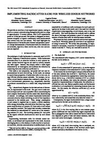
Results The result of this thesis work was a system to transmit compressed images from a camera node over a wireless connection to a database that could be access using the Internet. The compression rate varies depending on the content but is usually between 90% and 99% compared to the previous camera network. The system can handle several cameras and when more cameras are added they will be scheduled to take and transmit images at different times. Since it is expensive in terms of energy consumption to power up and power down the camera it will take a sequence of images each time it is powered up. These images are then reconstructed to a video clip at the base station. The number of images to take each time the camera powers up can be set as a parameter when the system is started. The first image in the sequence and the video clip is added to the database to be accessible over the Internet. A small testbed containing a solar-powered camera node and a base station was set up at the Brisbane site. This system was running stable for several days. Some sample images from this system are shown in figure 6.1 A paper based on this thesis work was accepted for the 6th International Conference on Information Processing in Sensor Networks (IPSN 2007). 24-27 April 2007, Cambridge (MIT Campus), Massachusetts, USA [25]. At this conference the system was also demonstrated. In this demonstration several cameras could be added to the network. Since power saving features was not used here and the cameras was always powered on it was possible to use very tight scheduling between cameras. The reason for this modification was to create a more interesting demonstration compared to the real system where nodes are put to sleep most of the time to save power.

31

32

Chapter 6. Results

Figure 6.1: Sample images taken by the wireless sensor network camera system.

Chapter 7

Conclusions The approach of first implementing an offline version in Linux for the image codec worked very well. By using this approach it was possible to test new ideas for codec techniques much more efficiently compared to when the codec was implemented on the DSP. During development bugfixing was also much faster on the Linux platform compared to the DSP platform. Once the codec was implemented on Linux the process of moving the encoder to the DSP and the decoder to the JAVA listener was done in a few days. The major problem was the different datatypes used on Linux compared to the DSP. The lack of pointers in Java did also cause some problems. This process could have been even simpler if the code on Linux would have been written more careful with portability in mind. The major components to implement were the DCT transform and the VLC and Huffman coding. The DCT transform had to be optimized and portable to run both on the DSP and on the Java listener. The algorithm used for DCT transform is one of the fastest available, however no low-level optimization of the code on the DSP was done. Currently encoding and transmission of an image takes in the order of one second. This will make it possible to only send very low framerate video. It should however be possible to enable high framerate video by optimize the code and reduce the resolution slightly. The implementation of the wireless communication on the FleckTM was done in TinyOS and NesC. This is a little different programming language and some time was required to get used to it. This work had a focus on the image coding for sensor networks. In future work it can be interesting to look more at the wireless communication in an image sensor network. The error control for images and video in wireless network usually requires a cross-layer design between the coding and the network. The overhead from the packet header is relatively large since the maximum packet size used in the system is small. Methods to reduce the packet header overhead are a possible future research topic. Another topic is on transport and routing layer when the bursty video or image data is mixed with the other sensor data. For future long-term research in this area distributed source coding certainly is interesting. This was a very interesting project since it involved work in both image processing and wireless communication. The project also had an applied approach. The system was implemented and tested in a real testbed.

33

34

Chapter 7. Conclusions

Chapter 8

Acknowledgements First I would like to thank my supervisor at CSIRO, Tim Wark, and my supervisor at Ume˚ a University, Jerry Eriksson, for their support and encouragement during this project. I would also like to thank all the people at the CSIRO Autonomous Systems Lab for making it a really friendly and interesting place to work; Peter Corke, Christopher Crossman, Michael Ung, Philip Valencia and Tim Wark to mention a few. I really enjoyed my time there.

35

36

Chapter 8. Acknowledgements

References [1] Ian F. Akyildiz, Tommaso Melodia, and Kaushik R. Chowdhury. A survey on wireless multimedia sensor networks. Comput. Networks, 51(4):921–960, 2007. [2] Tim Wark, Peter Corke, Pavan Sikka, Lasse Klingbeil, Ying Guo, Chris Crossman, Phil Valencia, Dave Swain, and Greg Bishop-Hurley. Transforming agriculture through pervasive wireless sensor networks. IEEE Pervasive Computing, 6(2):50– 57, 2007. [3] K.G. Langendoen, A. Baggio, and O.W. Visser. Murphy loves potatoes: Experiences from a pilot sensor network deployment in precision agriculture. In 14th Int. Workshop on Parallel and Distributed Real-Time Systems (WPDRTS), apr 2006. [4] Wei Zhang, George Kantor, and Sanjiv Singh. Integrated wireless sensor/actuator networks in an agricultural application. In Proceedings of the 2nd International Conference on Embedded Networked Sensor Systems, SenSys 2004, Baltimore, MD, USA, November 3-5, 2004, page 317. [5] Tim Wark, Chris Crossman, Wen Hu, Ying Guo, Philip Valencia, Pavan Sikka, Peter Corke, Caroline Lee, John Henshall, Julian O’Grady, Matt Reed, and Andrew Fisher. The design and evaluation of a mobile sensor/actuator network for autonomous animal control. In ACM/IEEE International Conference on Information Processing in Sensor Networks (SPOTS Track), April 25-27 2007. [6] Pei Zhang, Christopher M. Sadler, Stephen A. Lyon, and Margaret Martonosi. Hardware design experiences in zebranet. In Proceedings of the 2nd International Conference on Embedded Networked Sensor Systems, SenSys 2004, Baltimore, MD, USA, November 3-5, 2004, pages 227–238. [7] Wu-Chi Feng, Ed Kaiser, Wu Chang Feng, and Mikael Le Baillif. Panoptes: scalable low-power video sensor networking technologies. ACM Trans. Multimedia Comput. Commun. Appl., 1(2):151–167, 2005. [8] Purushottam Kulkarni, Deepak Ganesan, Prashant Shenoy, and Qifeng Lu. Senseye: a multi-tier camera sensor network. In MULTIMEDIA ’05: Proceedings of the 13th annual ACM international conference on Multimedia, pages 229–238, New York, NY, USA, 2005. ACM Press. [9] Georgiy Pekhteryev, Zafer Sahinoglu, Philip Orlik, and Ghulam Bhatti. Image transmission over ieee 802.15.4 and zigbee networks. In IEEE International Symposium on Circuits and Systems (ISCAS 2005), volume 4, pages 3539–3542, 23-26 May 2005. 37

38

REFERENCES

[10] Stephan Hengstler and Hamid K. Aghajan. Wisnap: A wireless image sensor network application platform. In 2nd International Conference on Testbeds & Research Infrastructures for the DEvelopment of NeTworks & COMmunities (TRIDENTCOM 2006), March 1-3, 2006, Barcelona, Spain. IEEE, 2006. [11] Haibo Li, Astrid Lundmark, and Robert Forchheimer. Image sequence coding at very low bit rates: a review. IEEE Transactions on Image Processing, 3(5):589–609, 1994. [12] Iso/iec 14496-2 information technology - coding of audio-visual objects. International Organization for Standardization, December 2001. Second edition. [13] Iso/iec 14496-10:2005 information technology – coding of audio-visual objects – part 10: Advanced video coding. International Organization for Standardization, 2005. [14] Bernd Girod, Anne Aaron, Shantanu Rane, and David Rebollo-Monedero. Distributed video coding. Proceedings of the IEEE, Volume: 93, Issue: 1:71– 83, January 2005. Invited Paper. [15] David Slepian and Jack K. Wolf. Noiseless coding of correlated information sources. IEEE Transactions on Information Theory, Volume: 19, Issue: 4:471– 480, July 1973. [16] Aaron D. Wyner and Jacob Ziv. The rate-distortion function for source coding with side information at the decoder. IEEE Transactions on Information Theory, Volume: 22, Issue: 1:1– 10, January 1976. [17] Rohit Puri, Abhik Majumdar, Prakash Ishwar, and Kannan Ramchandran. Distributed video coding in wireless sensor networks. Signal Processing Magazine, IEEE, 23(4):94–106, July 2006. [18] Jason Hill, Robert Szewczyk, Alec Woo, Seth Hollar, David Culler, and Kristofer Pister. System architecture directions for networked sensors. SIGPLAN Not., 35(11):93–104, 2000. [19] Crossbow Technology Inc. Mica2 data sheet. http://www.xbow.com/. [20] Joseph Polastre, Robert Szewczyk, and David Culler. Telos: enabling ultra-low power wireless research. In IPSN ’05: Proceedings of the 4th international symposium on Information processing in sensor networks, page 48, Piscataway, NJ, USA, 2005. IEEE Press. [21] Peter Corke, Shondip Sen, Pavan Sikka, Philip Valencia, and Tim Wark. 2-year progress report: July 2004 to june 2006. Commonwealth Scientific and Industrial Research Organisation (CSIRO). [22] Christoph Loeffler, Adriaan Lieenberg, and George S. Moschytz. Practical fast 1-d dct algorithms with 11 multiplications. In International Conference on Acoustics, Speech, and Signal Processing (ICASSP-89), volume 2, pages 988–991, Glasgow, UK, 23-26 May 1989. [23] Information technology - digital compression and coding of continuous-tone still images requirements and guidelines. ITU Recommendation T.81, 09 1992.

REFERENCES

39

[24] David Gay, Philip Levis, J. Robert von Behren, Matt Welsh, Eric A. Brewer, and David E. Culler. The nesc language: A holistic approach to networked embedded systems. In Proceedings of the ACM SIGPLAN 2003 Conference on Programming Language Design and Implementation, pages 1–11, June 9-11 2003. [25] Johannes Karlsson, Tim Wark, Philip Valencia, Michael Ung, and Peter Corke. Demonstration of image compression in a low-bandwidth wireless camera network. In The 6th International Conference on Information Processing in Sensor Networks (IPSN 2007)., Cambridge (MIT Campus), Massachusetts, USA., 24-27 April 2007.

40

REFERENCES

Appendix A

Huffman tables

41

42

Chapter A. Huffman tables

Category 0 1 2 3 4 5 6 7 8 9 10 11

Code length 2 3 3 3 3 3 4 5 6 7 8 9

Code word 000 010 011 100 101 110 1110 11110 111110 1111110 11111110 111111110

Table A.1: Table for luminance DC coefficient differences

Category 0 1 2 3 4 5 6 7 8 9 10 11

Code length 2 2 2 3 4 5 6 7 8 9 10 11

Code word 000 01 10 110 1110 11110 111110 1111110 11111110 111111110 1111111110 11111111110

Table A.2: Table for chrominance DC coefficient differences

43

Run/Size 0/0 (EOB) 0/1 0/2 0/3 0/4 0/5 0/6 0/7 0/8 0/9 0/A 1/1 1/2 1/3 1/4 1/5 1/6 1/7 1/8 1/9 1/A 2/1 2/2 2/3 2/4 2/5 2/6 2/7 2/8 2/9 2/A 3/1 3/2 3/3 3/4 3/5 3/6 3/7 3/8 3/9 3/A 4/1 4/2 4/3 4/4

Code length 4 2 2 3 4 5 7 8 10 16 16 4 5 7 9 11 16 16 16 16 16 5 8 10 12 16 16 16 16 16 16 6 9 12 16 16 16 16 16 16 16 6 10 16 16

Code word 1010 00 01 100 1011 11010 1111000 11111000 1111110110 1111111110000010 1111111110000011 1100 11011 1111001 111110110 11111110110 1111111110000100 1111111110000101 1111111110000110 1111111110000111 1111111110001000 11100 11111001 1111110111 111111110100 1111111110001001 1111111110001010 1111111110001011 1111111110001100 1111111110001101 1111111110001110 111010 111110111 111111110101 1111111110001111 1111111110010000 1111111110010001 1111111110010010 1111111110010011 1111111110010100 1111111110010101 111011 1111111000 1111111110010110 1111111110010111

Table A.3: Table for luminance AC coefficients (1 of 4)

44

Chapter A. Huffman tables

Run/Size 4/5 4/6 4/7 4/8 4/9 4/A 5/1 5/2 5/3 5/4 5/5 5/6 5/7 5/8 5/9 5/A 6/1 6/2 6/3 6/4 6/5 6/6 6/7 6/8 6/9 6/A 7/1 7/2 7/3 7/4 7/5 7/6 7/7 7/8 7/9 7/A 8/1 8/2 8/3 8/4 8/5 8/6 8/7 8/8

Code length 16 16 16 16 16 16 7 11 16 16 16 16 16 16 16 16 7 12 16 16 16 16 16 16 16 16 8 12 16 16 16 16 16 16 16 16 9 15 16 16 16 16 16 16

Code word 1111111110011000 1111111110011001 1111111110011010 1111111110011011 1111111110011100 1111111110011101 1111010 11111110111 1111111110011110 1111111110011111 1111111110100000 1111111110100001 1111111110100010 1111111110100011 1111111110100100 1111111110100101 1111011 111111110110 1111111110100110 1111111110100111 1111111110101000 1111111110101001 1111111110101010 1111111110101011 1111111110101100 1111111110101101 11111010 111111110111 1111111110101110 1111111110101111 1111111110110000 1111111110110001 1111111110110010 1111111110110011 1111111110110100 1111111110110101 111111000 111111111000000 1111111110110110 1111111110110111 1111111110111000 1111111110111001 1111111110111010 1111111110111011

Table A.4: Table for luminance AC coefficients (2 of 4)

45

Run/Size 8/9 8/A 9/1 9/2 9/3 9/4 9/5 9/6 9/7 9/8 9/9 9/A A/1 A/2 A/3 A/4 A/5 A/6 A/7 A/8 A/9 A/A B/1 B/2 B/3 B/4 B/5 B/6 B/7 B/8 B/9 B/A C/1 C/2 C/3 C/4 C/5 C/6 C/7 C/8 C/9 C/A

Code length 16 16 9 16 16 16 16 16 16 16 16 16 9 16 16 16 16 16 16 16 16 16 10 16 16 16 16 16 16 16 16 16 10 16 16 16 16 16 16 16 16 16

Code word 1111111110111100 1111111110111101 111111001 1111111110111110 1111111110111111 1111111111000000 1111111111000001 1111111111000010 1111111111000011 1111111111000100 1111111111000101 1111111111000110 111111010 1111111111000111 1111111111001000 1111111111001001 1111111111001010 1111111111001011 1111111111001100 1111111111001101 1111111111001110 1111111111001111 1111111001 1111111111010000 1111111111010001 1111111111010010 1111111111010011 1111111111010100 1111111111010101 1111111111010110 1111111111010111 1111111111011000 1111111010 1111111111011001 1111111111011010 1111111111011011 1111111111011100 1111111111011101 1111111111011110 1111111111011111 1111111111100000 1111111111100001

Table A.5: Table for luminance AC coefficients (3 of 4)

46

Chapter A. Huffman tables

Run/Size D/1 D/2 D/3 D/4 D/5 D/6 D/7 D/8 D/9 D/A E/1 E/2 E/3 E/4 E/5 E/6 E/7 E/8 E/9 E/A F/0 (ZRL) F/1 F/2 F/3 F/4 F/5 F/6 F/7 F/8 F/9 F/A

Code length 11 16 16 16 16 16 16 16 16 16 16 16 16 16 16 16 16 16 16 16 11 16 16 16 16 16 16 16 16 16 16

Code word 11111111000 1111111111100010 1111111111100011 1111111111100100 1111111111100101 1111111111100110 1111111111100111 1111111111101000 1111111111101001 1111111111101010 1111111111101011 1111111111101100 1111111111101101 1111111111101110 1111111111101111 1111111111110000 1111111111110001 1111111111110010 1111111111110011 1111111111110100 11111111001 1111111111110101 1111111111110110 1111111111110111 1111111111111000 1111111111111001 1111111111111010 1111111111111011 1111111111111100 1111111111111101 1111111111111110

Table A.6: Table for luminance AC coefficients (4 of 4)

47

Run/Size 0/0 (EOB) 0/1 0/2 0/3 0/4 0/5 0/6 0/7 0/8 0/9 0/A 1/1 1/2 1/3 1/4 1/5 1/6 1/7 1/8 1/9 1/A 2/1 2/2 2/3 2/4 2/5 2/6 2/7 2/8 2/9 2/A 3/1 3/2 3/3 3/4 3/5 3/6 3/7 3/8 3/9 3/A 4/1 4/2 4/3 4/4

Code length 2 2 3 4 5 5 6 7 9 10 12 4 6 8 9 11 12 16 16 16 16 5 8 10 12 15 16 16 16 16 16 5 8 10 12 16 16 16 16 16 16 6 9 16 16

Code word 00 01 100 1010 11000 11001 111000 1111000 111110100 1111110110 111111110100 1011 111001 11110110 111110101 11111110110 111111110101 1111111110001000 1111111110001001 1111111110001010 1111111110001011 11010 11110111 1111110111 111111110110 111111111000010 1111111110001100 1111111110001101 1111111110001110 1111111110001111 1111111110010000 11011 11111000 1111111000 111111110111 1111111110010001 1111111110010010 1111111110010011 1111111110010100 1111111110010101 1111111110010110 111010 111110110 1111111110010111 1111111110011000

Table A.7: Table for chrominance AC coefficients (1 of 4)

48

Chapter A. Huffman tables

Run/Size 4/5 4/6 4/7 4/8 4/9 4/A 5/1 5/2 5/3 5/4 5/5 5/6 5/7 5/8 5/9 5/A 6/1 6/2 6/3 6/4 6/5 6/6 6/7 6/8 6/9 6/A 7/1 7/2 7/3 7/4 7/5 7/6 7/7 7/8 7/9 7/A 8/1 8/2 8/3 8/4 8/5 8/6 8/7 8/8

Code length 16 16 16 16 16 16 6 10 16 16 16 16 16 16 16 16 7 11 16 16 16 16 16 16 16 16 7 11 16 16 16 16 16 16 16 16 8 16 16 16 16 16 16 16

Code word 1111111110011001 1111111110011010 1111111110011011 1111111110011100 1111111110011101 1111111110011110 111011 1111111001 1111111110011111 1111111110100000 1111111110100001 1111111110100010 1111111110100011 1111111110100100 1111111110100101 1111111110100110 1111001 11111110111 1111111110100111 1111111110101000 1111111110101001 1111111110101010 1111111110101011 1111111110101100 1111111110101101 1111111110101110 1111010 11111111000 1111111110101111 1111111110110000 1111111110110001 1111111110110010 1111111110110011 1111111110110100 1111111110110101 1111111110110110 11111001 1111111110110111 1111111110111000 1111111110111001 1111111110111010 1111111110111011 1111111110111100 1111111110111101

Table A.8: Table for chrominance AC coefficients (2 of 4)

49

Run/Size 8/9 8/A 9/1 9/2 9/3 9/4 9/5 9/6 9/7 9/8 9/9 9/A A/1 A/2 A/3 A/4 A/5 A/6 A/7 A/8 A/9 A/A B/1 B/2 B/3 B/4 B/5 B/6 B/7 B/8 B/9 B/A C/1 C/2 C/3 C/4 C/5 C/6 C/7 C/8 C/9 C/A

Code length 16 16 9 16 16 16 16 16 16 16 16 16 9 16 16 16 16 16 16 16 16 16 9 16 16 16 16 16 16 16 16 16 9 16 16 16 16 16 16 16 16 16

Code word 1111111110111110 1111111110111111 111110111 1111111111000000 1111111111000001 1111111111000010 1111111111000011 1111111111000100 1111111111000101 1111111111000110 1111111111000111 1111111111001000 111111000 1111111111001001 1111111111001010 1111111111001011 1111111111001100 1111111111001101 1111111111001110 1111111111001111 1111111111010000 1111111111010001 111111001 1111111111010010 1111111111010011 1111111111010100 1111111111010101 1111111111010110 1111111111010111 1111111111011000 1111111111011001 1111111111011010 111111010 1111111111011011 1111111111011100 1111111111011101 1111111111011110 1111111111011111 1111111111100000 1111111111100001 1111111111100010 1111111111100011

Table A.9: Table for chrominance AC coefficients (3 of 4)

50

Chapter A. Huffman tables

Run/Size D/1 D/2 D/3 D/4 D/5 D/6 D/7 D/8 D/9 D/A E/1 E/2 E/3 E/4 E/5 E/6 E/7 E/8 E/9 E/A F/0 (ZRL) F/1 F/2 F/3 F/4 F/5 F/6 F/7 F/8 F/9 F/A

Code length 11 16 16 16 16 16 16 16 16 16 14 16 16 16 16 16 16 16 16 16 10 15 16 16 16 16 16 16 16 16 16

Code word 11111111001 1111111111100100 1111111111100101 1111111111100110 1111111111100111 1111111111101000 1111111111101001 1111111111101010 1111111111101011 1111111111101100 11111111100000 1111111111101101 1111111111101110 1111111111101111 1111111111110000 1111111111110001 1111111111110010 1111111111110011 1111111111110100 1111111111110101 1111111010 111111111000011 1111111111110110 1111111111110111 1111111111111000 1111111111111001 1111111111111010 1111111111111011 1111111111111100 1111111111111101 1111111111111110

Table A.10: Table for chrominance AC coefficients (4 of 4)