Cellular Automata for Traffic Flow Modeling Saifallah Benjaafar, Kevin Dooley and Wibowo Setyawan Department of Mechanical Engineering University of Minnesota Minneapolis, MN 55455
Abstract In this paper, we explore the usefulness of cellular automata to traffic flow modeling. We extend some of the existing CA models to capture characteristics of traffic flow that have not been possible to model using either conventional analytical models or existing simulation techniques. In particular, we examine higher moments of traffic flow and evaluate their effect on overall traffic performance. The behavior of these higher moments is found to be surprising, somewhat counter-intuitive, and to have important important implications for design and control of traffic systems. For example, we show that the density of maximum throughput is near the density of maximum speed variance. Contrary to current practice, traffic should, therefore, be steered away from this density region. For deterministic systems, we found traffic flow to possess a finite period which is highly sensitive to density in a non-monotonic fashion. We show that knowledge of this periodic behavior to be very useful in designing and controlling automated systems. These results are obtained for both single and two lane systems. For two lane systems, we also examine the relationship between lane changing behavior and flow performance. We show that the density of maximum lane changing frequency occurs past the density of maximum throughput. Therefore, traffic should also be steered away from this density region.
1.
Introduction Traffic flow modeling is an important step in the design and control of transportation
systems. Despite this importance, existing literature has yet to offer a comprehensive model capable of capturing the richness and complexity of real traffic. The objective of this paper is to explore a new modeling paradigm, cellular automata (CA), which has has emerged in the last few years as a very promising alternative to existing traffic flow models [2, 7, 14, 16]. CA models have the distinction of being able to capture micro-level dynamics and relate these to macro level traffic flow behavior. This is in contrast with existing models, which are either aggregate in their treatment of traffic flow (macroscopic models) or detailed and limited in scope (microscopic models). Cellular automata models are capable of explicitly representing individual vehicle interactions and relating these interactions to macroscopic traffic flow metrics, such as throughput, travel time, and vehicle speed.
By allowing different vehicles to possess different driving behaviors
(acceleration/deceleration, lane change rules, reaction times, etc.), CA models can more adequately capture the complexity of real traffic. CA models, by being either deterministic or stochastic, can be more effective in accounting for the inherent variability in most real traffic. In turn, this allows us to characterize not only average values of flow metrics but also their higher moments (e.g., variance).
Finally, CA models are amenable to
representing both single and multi-lane traffic, which is particularly crucial for the modeling of highways. In this paper, we build on the pioneering work of Nagel and his colleagues [7, 8, 10, 11, 15] who were among the first to recognize the usefulness of cellular automata to traffic flow modeling. Their models have been extended by several others in the last few years [2, 5, 6 , 13, 14]. However, most of the existing models have focused on describing the relationship between the first moments of traffic flow measures. In this paper, we examine the behavior of higher moments of these metrics. We show that behavior of these higher moments to be not only surprising but also to have important implications for design and
-2-
control of traffic systems. For deterministic systems, we investigate the phenomenon of flow periodicity. We show that, in general, traffic flow is periodic with a finite period length. This finite period is found to be highly sensitive to traffic density in a nonmonotonic fashion. We show that knowledge of this periodic behavior can be very useful in designing and controlling automated roadway systems. The organization of the paper is as follows. In section 2, we provide a brief overview of existing traffic flow models and discuss some of their limitations. In section 3, we present a series of cellular automata models: deterministic single lane, stochastic single lane, and stochastic multi-lane, and discuss several interesting insights obtained from these models. In section 4, we briefly discuss the issue of time scaling as to CA-based computer simulation. Finally, in section 5, we present a discussion and conclusion.
2.
Traffic Flow Modeling in the Literature Traffic flow models can be divided into two major categories: microscopic and
macroscopic. Microscopic models describe traffic behavior as emerging from discrete entities interacting with each other. They range from simple analytical models, such as carfollowing models [4], to detailed simulation models, such as the FRESIM [3] and NETSIM [12] simulation software. Macroscopic models are concerned with describing the aggregate behavior of traffic by characterizing the fundamental relationships between vehicle speed, flow and density.
Example macroscopic models include input/output,
simple continuum, and higher order continuum [4]. A major limitation of the existing microscopic models (e.g., the car-following model) is that they assume uniform behavior for all vehicles. The models are deterministic and, therefore, cannot capture the inherent stochasticity in vehicle behavior in real traffic. Most microscopic models are also difficult to extend to multi-lane systems. A key limitation of macroscopic models is their aggregate nature.
Because they treat traffic flow as
continuous, they are incapable of capturing the discrete dynamics that arise from the interaction of individual vehicles. For example, modeling different driver behaviors with -3-
regard to acceleration/deceleration or lane changing is difficult.
Because they are
deterministic, these models can provide only average traffic flow metrics. Higher moments of throughput, travel time, and speed are impossible to characterize. Thus, the usefulness of most of these models is limited to characterizing the long run behavior of traffic flow and cannot be used for real time traffic analysis and control.
3. Cellular Automata for One-Lane Traffic Flow Cellular automata are mathematical idealizations of physical systems in which space and time are discrete, and physical quantities take on a finite set of discrete values. A cellular automaton consists of a regular uniform lattice, usually finite in extent, with discrete variables occupying the various sites. The state of a cellular automaton is completely specified by the values of the variables at each site. The variables at each site are updated simultaneously, based on the values of the variables in their neighborhood at the preceding time step, and according to a definite set of "local rule." (see [7] and [20] for a general review). Performance metrics are generally obtained through computer simulation of the evolution of the cellular automaton over time. Our initial traffic model is defined as a one dimensional array with L cells with closed (periodic) boundary conditions. This means that the total number of vehicles N in the system is maintained constant. Each cell (site) may be occupied by one vehicle, or it may be empty. Each cell corresponds to a road segment with a length l equal to the average headway in a traffic jam. Traffic density is given by ρ = N/L. Each vehicle can have a velocity from 0 to v max . The velocity corresponds to the number of sites that a vehicle advances in one iteration. The movement of vehicles through the cells is determined by a set of updating rules. These rules are applied in a parallel fashion to each vehicle at each iteration. The length of an iteration can be arbitrarily chosen to reflect the desired level of simulation detail. The choice of a sufficiently small iteration interval can thus be used to approximate a continuous time system. The state of of the system at an iteration is
-4-
determined by the distribution of vehicles among the cells and the speed of each vehicle in each cell. We use the following notation to characterize each system state: x(i): position of the ith vehicle, v(i): speed of ith vehicle, and g(i): gap between the ith and the (i+1)th vehicle (i.e., vehicle immediately ahead) and is given by g(i) = x(i + 1) - x(i) - 1.
3.1 Deterministic Cellular Automata In the deterministic single lane model, vehicle motion is determined by the following set of updating rules: 1. Acceleration of free vehicles: If v(i) < vmax and g(i) ≥ v(i) + 1, then v(i) = v(i) + 1. 2. Slowing down due to other vehicles: If v(i) > g(i) - 1, then v(i) = g(i). 3. Vehicle motion: Vehicle is advanced v(i) sites. Figure 1 shows the application of these three updating rules to an example system with 24 cells and 7 vehicles. These updating rules were first suggested by Nagel [7] and then used in many variations by others [5, 6, 14, 16]. Under these rules, all vehicles have identical behaviors and obey the same maximum speed. As we discuss later, these assumptions can be easily relaxed. For example, different vehicles could be assigned different maximum speeds. The tolerated gap between vehicles could also be made vehicle-dependent.
Erratic
acceleration and deceleration may also be included by introducing random accelerations and decelerations (see section 3.2). Throughout the simulation, we use a maximum speed vmax = 5 cells/iteration. We let each iteration correspond to one second. The length of each cell is taken to be 7.5 meters, which includes the average length of a vehicle and the gap between two neighboring vehicles in a traffic jam [7]. Therefore, vehicles assume the discrete speeds v0 = 0km/h, v1 = 27km/h, v2 = 54km/h, …, and vmax = 135km/h. This scaling is, however, not unique.
-5-
For example, we could have fixed the maximum allowable speed and then obtained the duration of each iteration. Other time scaling strategies are also possible (see section 4). It should be recognized that deterministic CA models are greatly simplified versions of real traffic. However, they can be useful in gaining insights into the fundamental behavior of traffic flow, insights that may not be easy to obtain without these simplifying assumptions. Deterministic CA can also be useful as a modeling paradigm for automated highway systems, where vehicle speeding and vehicle deceleration are externally controlled. Indeed, an automated highway system would operate very much like a deterministic cellular automaton with rules specifying the total number of vehicles allowed in the system and the set of allowable vehicle behaviors. Results from computer simulation of the above deterministic system are summarized in figures 2-6. The simulation is based on a system of 300 cells evaluated over 10,000 iterations (approximately 2.8 hours) for varying density levels. For each density level, various traffic flow measures were obtained (e.g., throughput, average speed, speed variance, traffic periodicity, etc.). A number of interesting observations can be made: • The model reproduces the familiar fundamental diagram of flow versus density - see Figure 2. Flow is linearly increasing with initial increases in traffic density (laminar flow). A maximum flow of 3000 vehicles/hour is achieved at ρmax = 0.1667, beyond which flow becomes linearly decreasing in density (back traveling start-stop waves). This behavior is consistent with empirical observations of actual traffic [4] (a more accurate approximation is provided by the stochastic version of the model presented in section 3.2). • In the laminar flow phase, average speed converges to the maximum speed v max . Average speed becomes a decreasing function of density for traffic densities larger than
ρmax - see Figure 3. These results are, again, not surprising and are consistent with available empirical data. However, what is surprising is the behavior of speed variance. As shown in Figure 4, there is a maximum variance density which occurs shortly after the maximum throughput density. Thus, the region of maximum flow is also the region of
-6-
maximum variance. Note that during the laminar flow phase, speed variance is negligible but starts to increase with the onset of maximum flow. The initial increase is fairly large creating a significant discontinuity in the "variance-density" function (for example, adding a single vehicle to a system with density ρ max, increases variance 19 times). High speed variance means that different vehicles in the system have widely varying speeds. It also means that a vehicle would experience frequent speed changes per trip through the system. In turn, this may result in higher trip travel time variance. In reality, this could also increase the probability of traffic accidents. Thus, it seems reasonable to attempt to steer traffic away from the density of maximum flow. A recommendation that is counter to prevailing practice where the objective is often to maximize flow. • Because we consider a deterministic and finite CA model with periodic boundaries, the corresponding traffic system is periodic in its system states.
That is, the number of
iterations necessary to bring back the same state is finite (Note: a state is defined by a distribution of vehicles among the cells and the vehicles' speeds). Figures 5 and 6 depict the behavior of the period length as a function of density for two example systems. Period length is negligible for densities below the maximum flow densities. However, the period length can be significant for higher densities. Surprisingly, period length is not monotonic in traffic density. In fact, either an increase or a decrease in period length may occur with an increase in density. More importantly, small changes in density could result in large fluctuations in period length. For example, for the system depicted in Figure 5, an increase in traffic density from 0.2 to 0.22 produces an increase in the period length from 300 to 18,300 (note: in each case, the simulation was run over a sufficient length to observe the full period). In practice, a traffic system with a small period length is more desirable since the number of states the system goes through is smaller, resulting in a system that is easier to predict and control. Finally, we should note that for a deterministic CA model, it is possible to obtain analytical expressions for average speed and average flow. Average speed in the laminar
-7-
flow phase is simply vmax, while in the back traveling phase, it is given by v = (1 - ρ )/ρ . Average flow can be calculated as j = ρ v. The maximum flow density occurs at the intersection of the two phases. This leads to ρmax = 1/(1 + vmax). However, obtaining analytical expressions for higher moments of flow or speed are difficult. It is also difficult to analytically characterize period length.
3.2 Stochastic Cellular Automata The deterministic CA model does not capture the inherent randomness in the behavior of vehicles in real traffic. In particular, it fails to account for non-deterministic acceleration and deceleration, inherent variability in vehicle speed, and vehicle over-reaction when slowing down. This stochasticity can be, in part, captured by adding a randomization rule to the three updating rules at each iteration of the CA model (see [20] for further details). The randomization rule is applied after the first two rules and results in reducing the speed of each vehicle by one with some probability p (i.e., if v > 0 then v = v - 1 with probability p, 0 ≤ p ≤ 1). Following this randomization step, all vehicles are advanced v cells. Results from computer simulation of the stochastic CA models are summarized in Figures 7-12. The simulation is conducted over 10,000 iterations, the first 1,000 of which are eliminated from consideration (transient period).
The results are similar to those
obtained for the deterministic case, with the important exception that flow, as a function of density, is not continuous during the back traveling phase (for densities that immediately follow ρ max, the initial reduction in flow is much more significant than it is for larger densities). This behavior is again consistent with observed real world traffic. Most of our previous observations can be generalized to the stochastic case. It is once again important to note that the density of maximum flow is in the region of the density of maximum speed variance. Therefore, operating traffic at lower densities should be pursued whenever possible.
For example, in our simulated system, operating at a density that reduces
maximum flow by 6% reduces speed variance by over 105%.
-8-
In Figures 10-12, the effect of uncertainty in vehicle behavior is examined. Three deceleration probabilities are compared: p = 0, 0.1 and 0.5. It is easy tro see that increased variability in vehicle behavior reduces throughput in the system. In particular. it reduces the maximum feasible throughput and the density at which this throughput is achieved. When variability is high (e.g., p = 0.5), the reduction can be significant. Variability also reduces average speed and the duration of the phase of laminar flow.
Note that, for high
variability, the average speed during the laminar flow phase is smaller the maximum feasible speed vmax .
Furthermore, variability decreases average speed and reduces the
density at which maximum speed variance occurs. However, it is interesting to note that partial reduction in variability (i.e., a smaller p) results in only limited reduction in speed variance. This means that the presence of any amount variability is sufficient to result in high speed variance. Our findings are consistent with those obtained by Nagel et al.who conducted somewhat similar experiments [10].
3.3 Stochastic Cellular Automata for Two-Lane Traffic Flow Most roadways do not consist of a single lane only. In fact, most highways provide two or more lanes. Despite this prevalence, existing literature offers few analytical models for multi-lane traffic. This can, in part, be explained by the difficulty of characterizing lane changing behavior, which requires the explicit modeling of discrete entities.
In this
section, we extend our single lane CA model to two lanes. We believe that CA models can be particularly useful in modeling multi-lane traffic since they can explicitly capture varying rules of lane changing. Our objective is to gain insights into the behavior of traffic on each lane and the the dynamics of lane changing under varying density levels. Our approach is to use a minimal set of acceleration, deceleration, and lane changing rules that are capable of yielding realistic macroscopic traffic behavior. Nagatani was the first to consider a CA model for two lane traffic [6]. His initial model was deterministic and used a vmax = 1. However, this model led to situations where blocks of several vehicles oscillate between lanes without any of the vehicles moving -9-
forward. This problem was later corrected by introducing randomness into lane changing. Building on Nagatani's model, Rickert et al. [13] considered a model with vmax ≥ 1. These models serve as the basis for the model we present here. While we use similar rules to Rickert et al. [13], the experiments we conduct, especially those pertaining to variance, are different from those discussed in [13]. The updating rules from the single lane model are extended as follows.
At the
beginning of each iteration, vehicles check whether a lane change is desirable or not. This is done according to a set of lane changing rules. Once all lane changes are made, the updating rules from the single lane model are applied independently to each lane.
In
modeling lane changing behavior, we make two important assumptions: (1) during lane changeover, only transversal movement are allowed (i.e., vehicles do not advance) and (2) once a vehicle changes lanes, it remains in that lane until it becomes more desirable to move back to the other lane (i.e., vehicles do not always return to the right lane). The lane changing rules, which are applied in parallel to each vehicle, can be summarized as follows: 1. Look ahead: a vehicle looks ahead to see if the existing gap can accommodate its current speed - i.e., v(i) ≤ g(i). If not, then go to rule 2. 2. Look sideways: the vehicle looks at the other lane to see if the forward gap on that lane will allow it to maintain or increase its current speed. 3. Look back: the vehicle looks at the other lane to see if the backward gap on that lane is large enough not to affect the speed of other vehicles. If so, then perform a lane change. Randomness can be introduced into lane changing, by associating a probability, pchange, with whether a change is actually effected, once it is deemed possible, or not. At the cost of additional rules, a preference for the original lane (e.g., right lane) can also be modeled. Simulation results of example systems are shown in Figures 13-16. The results were obtained for L = 300, p = 0.5, and pchange = 1. Because of our symmetry assumption in treating both lanes, traffic flow characteristics on both lanes are identical. Lane changing
-10-
behavior is depicted in Figure 15. It is interesting to note that maximum lane changing frequency occurs long after the criticial density of maximum throughput.
It is also
interesting to observe that more frequent lane changing does not correspond to greater speed variance. In fact, the density of maximum speed variance is in the vicinity of the density of maximum throughput. In real traffic, frequent lane changing is undesirable since it increases the likelihood of accidents. Therefore, traffic should be steered away from the density of maximum lane changing frequency. Figures 17-19 provide a comparison between one lane and two lane systems. To allow for a fair comparison between the two systems, the one lane system has 300 cells and the two lane system has two lanes with 150 cells each.
It is interesting to observe that,
although both systems have the same number of cells and operate at the same density, the two lane system achieves a total throughput that is double that of the one lane system. Also, despite this higher throughput, average speed and speed variance are almost the same in both systems.
4. Time Scaling As we mentioned in section 3, various time scaling strategies are possible. Nagel and Schreckenberg [11], among others, identified three different schemes for interpreting the simulation time scales. The first scheme is based on a maximum allowable speed and a predefined length of each cell. These are then used to compute the duration of each iteration. A variation on this scheme was used in this paper. The second scheme scales the model using the flow-density diagram. Using the known maximum roadway capacity (e.g., freeways have a maximum capacity of about 2000 vehicles/hour/lane), the corresponding length of an iteration can be calculated. In our example stochastic single lane system (p = 0.5), the maximum throughput is 0.38 vehicles/iteration. Thus, one iteration corresponds to 0.68 seconds. The third scheme uses the known value for the velocity of the back-traveling phase (e.g., a value of about 15 km/h has been measured for freeways [12]) to obtain the length of an iteration. In our simulated stochastic system, the -11-
simulated maximum velocity during the back traveling phase is 0.38 sites/iteration, which means that one iteration corresponds again to 0.68 seconds. Other time scaling schemes may also be possible. However, the nature of the macroscopic insights obtained from the simulation are unaffected by these time scales.
5
Discussion and Conclusion In this paper, we explored the usefulness of cellular automata to traffic flow modeling.
We extended some of the existing CA models to capture interesting characteristics of traffic flow that have not been possible to model using either conventional analytical models or existing simulation techniques. Using CA models, we were able to examine higher moments of traffic flow, which we show to behave in a rather unexpected fashion. For example, we showed that the density area of maximum throughput is also the density area of maximum speed variance. For deterministic systems, we found traffic flow to possess a finite period which is highly sensitive to density in a non-monotonic fashion. Knowledge of this periodic behavior can be very useful in designing and controlling automated systems, since shorter periods mean fewer system states and, therefore, greater traffic predictability. We also showed that CA models are more amenable to modeling multi-lane traffic. Lane changing rules and behavior can be explicitly accounted for in the model. The impact of these rules and behaviors becomes then easier to examine. In our preliminary study, we showed that the density of maximum lane changing frequency occurs after the density of maximum throughput. This means that lane changing does little to increase throughput. Since more frequent lane changing means an increase in the likelihood of traffic accidents, traffic should be operated at lower densities (e.g., through ramp meters). In fact, the desired density should be smaller than both the density of maximum lane changing and maximum throughput. This will ensure traffic with few lane changes and with a small speed variance.
-12-
The models we presented are only an initial attempt at gaining insight into the discrete behavior of traffic flow (and its impact on microscopic performance). Our basic models should now be extended to more realistic traffic settings. For example, vehicles do not necessarily behave in a homogeneous fashion.
Different vehicles could be assigned
different rules for acceleration, deceleration, and lane changing. In Multi-lane systems, the lane symmetry assumption should be relaxed to allow for different lane preferences for different vehicles. Our current model is based on a single entry/single exit system. Future work should include systems with multiple entries and exits.
Acknowledgements This research was supported by the U.S. Department of Transportation under grant No. USDOT/DTRS93-G-0017 and the University of Minnesota Intelligent Transportation Systems (ITS) Institute.
-13-
References [1] Biham, O., Middleton, A. and D. Levine, "Self-Organization and a Dynamical Transition in Traffic Flow Models," Physical Review A, Vol. 46, No. 10, pp. 6124-6127, 1992. [2] Blue, V., Bonetto, F. and M. Embrechts, "A Cellular Automata of Vehicular Self Organization and Nonlinear Speed Transitions," Transportation Research Board Annual Meeting, Washington, DC, 1996. [3] FRESIM User Guide, Version 4.5, Federal Highway Administration, US Department of Transportation, Washington, DC, 1994. [4] Gerlough, D. L. and M. J. Hunber, Traffic Flow Theory - A Monograph, Transportation Research Board National research Council, Special Report 165, 1991. [5] Nagatani, T., "Jamming Transition in the Traffic Flow Model with Two-Level Crossings," Physical Review E, Vol. 48, No. 5, pp. 3290-3294, 1993. [6] Nagatani, T., "Self Organization and Phase Transition in the Traffic Flow Model of a Two-Lane Roadway," Journal of Physics A, Vol. 26, pp. 781-787, 1993. [7] Nagel, K., "Particle Hopping Models and Traffic Flow Theory," Physical Review E," Vol. 3, No. 6, pp. 4655-4672, 1996. [8] Nagel, K., Barrett, C. L. and M. Rickert, "Parallel Traffic Micro-Simulation by Cellular Automata," Transportation Research C, submitted, 1996. [9] Nagel, K. and H. Hermann, "Deterministic Models for Traffic Jams," Physica A, Vol. 199, pp. 254-263, 1993. [10] Nagel, K. and S. Rasmussen, "Traffic at the Edge of Chaos," Proceedings of the Fourth International Workshop on the Synthesis and Simulation of Living Systems, MIT Press, pp. 222-235, 1994. [11] Nagel, K. and M. Schreckenberg, "A cellular Automaton Model for Freeway Traffic," Journal de Physique, Vol. 2, pp. 2221-2229, 1992. [12] Rathi, A. K. and and A. J. Santiago, "The New NETSIM Simulation Program," Traffic Engineering and Control, pp. 317-320, 1990. [13] Rickert, M., Nagel, K., Schreckenberg, M. and A. Latour, "Two Lane Traffic Simulations using Cellular Automata," Physica A, submitted, 1995. [14] Schadschneider, A. and M. Schreckenberg, "Cellular Automaton Models and Traffic Flow," Journal of Physics A, Vol. 26, pp. 679-683, 1993. [15] Schreckenberg, M., schreckenberg, A., Nagel, K. and N. Ito, "Discrete Stochastic Models for Traffic Flow, Physical Review E, Vol. 51, No. 4, pp 2939-2949, 1995. [16] Villar, L. and A. de Souza, "Cellular Automata Models for General Traffic Conditions on a Line," Physica A, Vol. 211, pp. 84-92, 1994.
-14-
[17] Wolfram, S., Theory and Applications of Cellular Automata, World Scientific, New York, NY, 1986.
-15-
4
Iteration T + 2
Iteration T + 1
3
Iteration T
-16-
2
3
Vehicle speed 2
2 3
3
1
3
1
1
2
Figure 1 Example CA Model Evolution
2
2
2
1
3
2
3
3