Commun. Theor. Phys. (Beijing, China) 51 (2009) pp. 595–599 c Chinese Physical Society and IOP Publishing Ltd

Vol. 51, No. 4, April 15, 2009

Station Model for Rail Transit System Using Cellular Automata∗ XUN Jing,† NING Bin, and LI Ke-Ping State Key Laboratory of Rail Traffic Control and Safety, Beijing Jiaotong University, Beijing 100044, China

(Received June 23, 2008; Revised September 19, 2008)

Abstract In this paper, we propose a new cellular automata model to simulate the railway traffic at station. Based on NaSch model, the proposed station model is composed of the main track and the siding track. Two different schemes for trains passing through station are considered. One is the scheme of “pass by the main track, start and stop by the siding track”. The other is the scheme of “two tracks play the same role”. We simulate the train movement using the proposed model and analyze the traffic flow at station. The simulation results demonstrate that the proposed cellular automata model can be successfully used for the simulations of railway traffic. Some characteristic behaviors of railway traffic flow can be reproduced. Moreover, the simulation values of the minimum headway are close to the theoretical values. This result demonstrates the dependability and availability of the proposed model. PACS numbers: 02.70.-c, 89.40.-a

Key words: cellular automata (CA), multi-platform station, moving block system (MBS)

1 Introduction Nowadays, with the rapid development of science and technologies, many restrictions on the application of Moving Block System (MBS) have been solved. More and more transit systems with MBS have been constructed and put into operation. However, the theory study on MBS falls far behind the project application. Recently there have been some developments on the theory research on MBS. Some scholars analyzed the delay propagation of train running with MBS.[1−4] Goossens[5] analyzed the line planning problems, and other scholars did researches on control and adjustment of train following operation,[6] automatic train operation,[7,8] carrying capacity of line[9] and real-time traffic optimization in railways.[10] The previous researches are mainly based on the classic mathematical methods. Few of them modeled the principle of train-following operation. Ning Bin and Li Ke-Ping[11,12] extended the NaSch model and proposed an improved model of train-following. Zhou Hua-Liang and Gao ZiYou[13] simulated the traffic phenomenon of delay propagation using a cellular automaton model for moving-like block system. In Ref. [14], a model which was extended to the railway network was proposed. However, the models proposed in Ref. [14] just simply treated station as a cell, namely only one train can occupy the station at one time. This assumption increases the applicability of the model and facilitates the simulation. At the same time, it directly influences the simulation results. Actually in the rail transit system, a station is composed of several platforms, and at one time more than one train can be allowed to enter the station. On the basis of Ref. [14], we propose a station model linked by 2 one-way lines in each direction, traversed by trains with different types and speeds. So the station model is ∗ The

composed of the main track and the siding track in the uplink and downlink. This station model represents the basic type of railway station. The paper is organized as follows: We introduce the proposed model in Sec. 2, and use the proposed model to simulate an example of railway network in Sec. 3. The analytical results and discussions are described in Sec. 4. Finally, the conclusions of this approach are presented.

2 Simulation Model 2.1 NaSch Model Nagel and Schreckenberg developed a one-dimensional probabilistic CA model (called NaSch model), which is a model of traffic flow on a single-lane.[14] In NaSch model, the road is divided into L cells numbered by i = 1, 2, . . . , L, and time is discrete. Each site can be either empty or occupied by a vehicle with integer speed Vi = 0, 1, . . . , Vmax , where Vmax is the maximum speed. Xi (t) is the position where vehicle i is at time t, and gapi (t) = Xi+1 (t) − Xi (t) − 1 expresses the gap between vehicle i and i + 1 at time t. The underlying dynamics of NaSch model are governed by the updated rules applied at discrete time steps. All sites are simultaneously updated according to four successive steps. (i) Acceleration Vi (t + 1) → min(Vi (t) + 1, Vmax ) ; (ii) Slowing down Vi (t + 1) → min(Vi (t), gapi (t)) (iii) Randomization Vi (t + 1) → max(Vi (t) − 1, 0) ; (Decrease Vi (t) by 1 with randomization probability q if Vi (t) > 0);

project supported by National Natural Science Foundation of China under Grant Nos. 60634010 and 60776829 and Key Technology Research of Train Control System, and Urban Rail Transit Automation and Control Beijing Municipal Government Key Laboratory † Corresponding author, E-mail: [email protected]

596

XUN Jing, NING Bin, and LI Ke-Ping

This step is ignored in our proposed model, i.e., the randomization probability q is q = 0. (iv) Movement Xi (t + 1) → Xi (t) + Vi (t + 1) .

yellow and double yellow, which represent different types of permission speed in which train can enter the station. The algorithms when a train enters the improved station are changed as follows: If

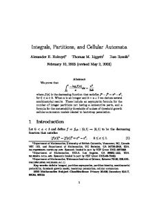
2.2 Proposed Station Model Based on Ref. [14], we improve the station model that doesn’t treat itself as a cell simply. It is extended to a station with main and siding tracks, as shown in Fig. 1. In the station model, we have two schemes: One is scheme A that a train passes by the main track and stops by the siding track. The other is scheme B that two tracks play the same role and a train can stop by either and pass by the main track. If a train from direction A stops by the siding track, the route from signal S1 to signal S7 will be arranged unless it is occupied. If a train from direction A stops by the main track, the route from signal S1 to signal S5 will be arranged unless it is occupied. If a train from direction A passes by the main track, the route from signal S1 to signal S9 shall be arranged unless it is occupied. In Fig. 1, signal S1 and S10 can light in 4 colors, green, red,

Fig. 1

Vol. 51

Si = Green T rack occupation = T rack main Station state = P ass

Elseif

Si = Y ellow double T rack occupation = T rack siding Station state = Stop

Elseif

Si = Y ellow T rack occupation = T rack main Station state = Stop

Elseif

Si = Red T rack occupation = N ull Station state = W ait

End

Station map.

In the above, Si is the aspect of signal Si , Track occupation is the track occupied by the next train and Station state is the state of the next train. Track main stands for the main track of station and Track siding stands for the siding track of station. The interstation train-following algorithms are same to the ones in Ref. [14]. In order to compare simulation results with field measurements, one cellular automata iteration roughly corresponds to 1 second, and the length of a cell is approximately 5 m. This means, e.g., that Vmax = 10 cell/update corresponds to Vmax = 180 km/h.

3 Simulations We apply the model proposed in this paper to simulate an example of railway network, which is depicted in Fig. 2. This example of railway network includes 6 stations, 4 major lines, i.e. BC, BF, CD and DF, and 2 minor lines, i.e. AB and DE. Two types of train have been taken into account, i.e., the high-speed trains with the maximum speed Vmax = 10 and the conventional trains with Vmax = 6. In

Fig. 2, there are 6 stations, A, B, C, D, E, and F. Station D is the improved station. The lengths of the lines AB, BC, CD, BE, CE, and EF are respectively set to be AB = 150, BC = 250, CD = 200, DE = 400, DF = 200, and BF = 250. The length of the computational time is taken as T = 1000. Table 1 gives the train routes and daily train numbers. The train will departure the first station (Station A or E) successively with interval Ts . The train will disappear when it arrives at its destination, i.e. the boundary condition for our proposed CA model is open. There is a high-speed train every 4 conventional trains. There is also dwell time at each station in Table 1. The parameters used in the simulation are as follows: (i) The train acceleration and deceleration a = 1; (ii) The ratio of the high-speed train to the conventional train p = 0.25; (iii) The safety protection distance Ls = 65; (iii) The interval of departure Ts is different with different stations.

No. 4

Station Model for Rail Transit System Using Cellular Automata

Table 1 Type

Route

Number

High-speed

A-B-E

High-speed

E-B-A

597

Rain Routes and Dwell Time. Dwell Time Station A

Station B

Station C

Station D

Station E

4

10

10

10

4

10

10

10

Conventional

A-B-C-D-E

16

10

10

10

10

10

Conventional

E-D-C-B-A

16

10

10

10

10

10

when station C is occupied by the No. 118 conventional train then overtakes at the station D, where the No. 118 conventional train stops at the siding track. The simulation results demonstrate that the proposed model can basically reflect the main character of the traffic flow at station.

4 Discussions Fig. 2

An example of railway network.

Fig. 3

Schedule.

In the previous simulations, we discussed the influence on the delay at station D.

Fig. 5 Arrival delay with dwell time for Ts = 30, Ls = 65, a = 1, Vmax = 10, and p = 0.5.

Fig. 6 Arrival delay with interval of departure for Ts = 40, Ls = 65, a = 1, Vmax = 10, and p = 0.5. Fig. 4

Schedule ( a part of Fig. 3).

The schedule in Figs. 3 and 4 displays the simulation results between station A and station E. We can see that the No. 120 high-speed train has to wait behind station C

Figure 5 and 6 show the arrival delay behind station D. The arrival delay is PM (ti − t0i ) Davg = i=1 M

598

XUN Jing, NING Bin, and LI Ke-Ping

where ti is the i-th train’s actual arrive time at station D, t0i is the i-th train’s arrive time at station D without any delay and M is the total number of trains in the simulation. According to the record for the two schemes in Fig. 5, the delay before station D increases as the dwell time Td increases. The delay firstly appears at Td = 49 with scheme A. The delay appears at Td = 57 with scheme B. The delay with scheme B appears later than the one with scheme A and the average delay is less than the one with scheme A. As shown in Fig. 6, for the two schemes, the delay before station D decreases as the interval of departure Ts increases. The delay firstly disappears at Ts = 23 with scheme B. The delay disappears at Ts = 27 with scheme A. The delay with scheme B disappears earlier than that with scheme A, and the average delay is less than that with scheme A. In sum, the delay with scheme A is more than that with scheme B.

Vol. 51

In railway traffic, the safety is an important factor. If a train runs under a limited speed, the following train should keep a safety protection distance with the frontal train. It is a dangerous situation that two train run too close. In Fig. 8, the train decelerates or accelerates for several times. Sometimes the train moves with Vmax = 10, sometimes it moves with a lower speed, i.e., Vn = 6 in order to keep under the limited speed. In order to demonstrate the dependability and availability of the proposed model, we compare the simulation results with the theoretical results. The headway is an important parameter in railway traffic system. The definition of headway is the time interval that two successive trains pass a same site at a station. In Ref. [15], two theoretical formulae were proposed. For different maximum speed, minimum p headway is calculated by different formula. If Vmax ≥ 2(Ls + Lt )/a, the minimum headway is r 2(Ls + Lt ) Vmax + tan + , (1) Hmin = a b where Lt is the train length, b is the train deceleration and tan is the system response time (tan = 0 because we didn’t consider the effect caused by tan in the proposed model). p If Vmax ≤ 2(Ls + Lt )/a, the minimum headway is Hmin =

2 Vmax 2a(Ls + Lt ) + Vmax + tan + . 2aVmax b

(2)

Fig. 7 A diagram displaying the velocity and distance of one train for Td = 30 and Vmax = 10.

As shown in Fig. 7, a train stops not only at a station but also at lines, especially near the station. That is because some frontal trains have already occupied the platform. The next train has to wait behind the station. This delay will propagate and it should be avoid as much as possible.

Fig. 9 Comparison between the simulation values and theoretical values.

Fig. 8 A diagram displaying the velocity and time of one tracked train for Td = 30 and Vmax = 10.

The comparison between the simulation results and the theoretical results is shown in Fig. 9. The dotted line denotes the simulation values using the proposed model, and the solid line denotes the theoretical values calculated by Eqs. (1) and (2). From Fig. 9, we can see that the simulation values of the minimum time headway are close to the theoretical values. At low speed region, the simulation results and theoretical results nearly equal. And there is a margin at high speed region, where the simulation values are lower than the theoretical values. Furthermore, there

No. 4

Station Model for Rail Transit System Using Cellular Automata

is a minimum point of the time headway at the maximum speed. It is at about Vmax = 6 cells/update, i.e., Vmax = 108 km/h. This result demonstrates the dependability and availability of the model.

5 Conclusions In conclusions, we propose a new model in which station with multiplatform is considered. Some characteristic behaviors of railway traffic flow can be reproduced. The

References [1] H. Takeuchi, U. Goodman, and S. Sone, IEE Proc. Electr. Power Appl. 150 (2003) 483. [2] M. Zhao, Ph.D. Thesis, Northern Jiaotong University, Beijing (1996) p. 70 (in Chinese). [3] L.E. Meester and S. Muns, Transpn. Res. B 41 (2007) 218. [4] J. Yuan and I.A. Hansen, Transpn. Res. B 41 (2007) 202. [5] J.W. Goossens, S.V. Hoesel, and L. Kroon, European Journal of Operational Research 168 (2006) 403. [6] Y.L. Zhan, P. Li, L. Jia, and Y.E. Yang, Journal of System Simulation 16 (2004) 2258 (in Chinese). [7] L.J. Huang and T. Tao, Journal of Northern Jiaotong Univercity 26 (2002) 36 (in Chinese). [8] T. Tao and L.J. Huang, Journal of the China Railway Society 25 (2002) 99 (in Chinese).

599

proposed model can simulate complicated phenomena of railway traffic flow, such as overtaking. The delay will increase as the dwell time increases, and it will decrease as the interval of departure at the original station increases. In the station which is considered, the delay for the scheme A is more than the delay for the scheme B. The simulation values of the minimum headway are close to the theoretical values. This result demonstrates the dependability and availability of the proposed model.

[9] Y. Zhang, Ph.D. Thesis, Northern Jiaotong University, Beijing (1998) p. 101 (in Chinese). [10] M. Mazzarello and E. Ottaviani, Transpn. Res. B 41 (2007) 246. [11] K.P. Li, Z.Y. Gao, and B.J. Ning, Comp. Phys. 209 (2005) 179. [12] B. Ning, K.P. Li, and Z.Y. Gao, Int. J. Mod. Phys. 16 (2005) 1793. [13] H.L. Zhou, Z.Y. Gao, and K.P. Li, Acta Phys. Sin. 55 (2006) 1706 (in Chinese). [14] J. Xun, B. Ning, and K.P. Li, Acta Phys. Sin. 56 (2007) 5158 (in Chinese). [15] L.Y. Luo and W.Q. Wu, China Railway Science 26 (2006) 119 (in Chinese).