Parallel Cellular Automata: A Model Program for Computational Science∗ (1993)
We develop a generic program for parallel execution of cellular automata on a multicomputer. The generic program is then adapted for simulation of a forest fire and numerical solution of Laplace’s equation for stationary heat flow. The performance of the parallel program is analyzed and measured on a Computing Surface configured as a matrix of transputers with distributed memory.
1
Introduction
This is one of several papers that explore the benefits of developing model programs for computational science (Brinch Hansen 1990, 1991a, 1991b, 1992a). The theme of this paper is parallel cellular automata. A cellular automaton is a discrete model of a system that varies in space and time. The discrete space is an array of identical cells, each representing a local state. As time advances in discrete steps, the system evolves according to universal laws. Every time the clock ticks, the cells update their states simultaneously. The next state of a cell depends only on the current state of the cell and its nearest neighbors. In 1950 John von Neuman and Stan Ulam introduced cellular automata to study self-reproducing systems (von Neumann 1966; Ulam 1986). John Conway’s game of Life is undoubtedly the most widely known cellular automaton (Gardner 1970, 1971; Berlekamp 1982). Another well known automaton simulates the life cycles of sharks and fish on the imaginary planet ∗ P. Brinch Hansen, Parallel Cellular Automata: A model program for computational science. Concurrency—Practice and Experience 5, 5 (August 1993), 425–448. Copyright c 1993, John Wiley & Sons, Ltd. Revised version. °
1
2
PER BRINCH HANSEN
Wa-Tor (Dewdney 1984). The numerous applications include forest infestation (Hoppensteadt 1978), fluid flow (Frisch 1986), earthquakes (Bak 1989), forest fires (Bak 1990) and sandpile avalanches (Hwa 1989). Cellular automata can simulate continuous physical systems described by partial differential equations. The numerical solution of, say, Laplace’s equation by grid relaxation is really a discrete simulation of heat flow performed by a cellular automaton. Cellular automata are ideally suited for parallel computing. My goal is to explore programming methodology for multicomputers. I will illustrate this theme by developing a generic program for parallel execution of cellular automata on a multicomputer with a square matrix of processor nodes. I will then show how easy it is to adapt the generic program for two different applications: (1) simulation of a forest fire, and (2) numerical solution of Laplace’s equation for stationary heat flow. On a Computing Surface with transputer nodes, the parallel efficiency of these model programs is close to one.
2
Cellular Automata
A cellular automaton is an array of parallel processes, known as cells. Every cell has a discrete state. At discrete moments in time, the cells update their states simultaneously. The state transition of a cell depends only on its previous state and the states of the adjacent cells. I will program a two-dimensional cellular automaton with fixed boundary states (Fig. 1). The automaton is a square matrix with three kinds of cells: 1. Interior cells, marked “?”, may change their states dynamically. 2. Boundary cells, marked “+”, have fixed states. 3. Corner cells, marked“−”, are not used. Figure 2 shows an interior cell and the four neighbors that may influence its state. These five cells are labeled c (central), n (north), s (south), e (east), and w (west). The cellular automaton will be programmed in SuperPascal (Brinch Hansen 1994). The execution of k statements S1 , S2 , . . . , Sk as parallel processes is denoted parallel S1 |S2 | · · · |Sk end
PARALLEL CELLULAR AUTOMATA
− + + + + + + −
+ ? ? ? ? ? ? +
+ ? ? ? ? ? ? +
+ ? ? ? ? ? ? +
+ ? ? ? ? ? ? +
+ ? ? ? ? ? ? +
+ ? ? ? ? ? ? +
3
− + + + + + + −
Figure 1 A cellular automaton.
n w c e s Figure 2 Adjacent cells.
The parallel execution continues until every one of the k processes has terminated. The forall statement forall i := 1 to k do S(i)
is equivalent to parallel S(1)|S(2)| · · · |S(k) end
I assume that parallel processes communicate through synchronous channels only. The creation of a new channel c is denoted open(c)
The input and output of a value x through a channel c are denoted receive(c,x)
send(c,x)
4
PER BRINCH HANSEN
A cellular automaton is a set of parallel communicating cells. If you ignore boundary cells and communication details, a two-dimensional automaton is defined as follows: forall i := 1 to n do forall j := 1 to n do cell(i,j)
After initializing its own state, every interior cell goes through a fixed number of state transitions before outputting its final state: initialize own state; for k := 1 to steps do begin exchange states with adjacent cells; update own state end; output own state
The challenge is to transform this fine-grained parallel model into an efficient program for a multicomputer with distributed memory.
3
Initial States
Consider a cellular automaton with 36 interior cells and 24 boundary cells. In a sequential computer the combined state of the automaton can be represented by an 8 × 8 matrix, called a grid (Fig. 3). For reasons that will be explained later, the grid elements are indicated by 0’s and 1’s. Figure 4 shows the initial values of the elements. The boundary elements have fixed values u1 , u2 , u3 and u4 . Every interior element has the same initial value u5 . In general, a grid u has n×n interior elements and 4n boundary elements: const n = ...; type state = (...); row = array [0..n+1] of state; grid = array [0..n+1] of row; var u: grid;
Since the possible states of every cell vary from one application to another, I deliberately leave them unspecified. The grid dimension n and the initial states u1 , u2 , u3 , u4 and u5 are also application dependent. On a sequential computer, the grid is initialized as follows:
PARALLEL CELLULAR AUTOMATA
− 1 0 1 0 1 0 −
1 0 1 0 1 0 1 0
0 1 0 1 0 1 0 1
1 0 1 0 1 0 1 0
0 1 0 1 0 1 0 1
1 0 1 0 1 0 1 0
0 1 0 1 0 1 0 1
5
− 0 1 0 1 0 1 −
Figure 3 A square grid.
u1
u4
u5
u3
u2 Figure 4 Initial values.
for i := 0 to n + 1 do for j := 0 to n + 1 do u[i,j] := initial(i,j)
Algorithm 1 defines the initial value of the element element u[i, j]. The values of the corner elements are arbitrary (and irrelevant).
4
Data Parallelism
For simulation of a cellular automaton, the ideal multicomputer architecture is a square matrix of identical processor nodes (Fig. 5). Every node is connected to its nearest neighbors (if any) by four communication channels.
6
PER BRINCH HANSEN
function initial(i, j: integer): state; begin if i = 0 then initial := u1 else if i = n + 1 then initial := u2 else if j = n + 1 then initial := u3 else if j = 0 then initial := u4 else initial := u5 end; Algorithm 1
Figure 5 Processor matrix.
Figure 6 shows a grid with 36 interior elements divided into 9 subgrids. You now have a 3×3 matrix of nodes and a 3×3 matrix of subgrids. The two matrices define a one-to-one correspondence between subgrids and nodes. I will assign each subgrid to the corresponding node and let the nodes update the subgrids simultaneously. This form of distributed processing is called data parallelism. Every processor holds a 4 × 4 subgrid with four interior elements and eight boundary elements (Fig. 7). Every boundary element holds either an interior element of a neighboring subgrid or a boundary element of the entire grid. (I will say more about this later.)
PARALLEL CELLULAR AUTOMATA
− 1 0 1 0 1 0 −
1 0 1 0 1 0 1 0
0 1 0 1 0 1 0 1
1 0 1 0 1 0 1 0
0 1 0 1 0 1 0 1
1 0 1 0 1 0 1 0
0 1 0 1 0 1 0 1
7
− 0 1 0 1 0 1 −
Figure 6 A subdivided grid.
− 1 0 −
1 0 1 0
0 1 0 1
− 0 1 −
Figure 7 A subgrid.
5
Processor Nodes
With this background, I am ready to program a cellular automaton that runs on a q × q processor matrix. The nodes follow the same script (Algorithm 2). A node is identified by its row and column numbers (qi , qj ) in the processor matrix, where 1 ≤ qi ≤ q and 1 ≤ qj ≤ q Four communication channels, labeled up, down, left, and right, connect a node to its nearest neighbors (if any). Every node holds a subgrid with m × m interior elements and 4m boundary elements (Fig. 7): const m = ...; type subrow = array [0..m+1] of state; subgrid = array [0..m+1] of subrow;
8
PER BRINCH HANSEN
procedure node(qi, qj, steps: integer; up, down, left, right: channel); var u: subgrid; k: integer; begin newgrid(qi, qj, u); for k := 1 to steps do relax(qi, qj, up, down, left, right, u); output(qi, qj, right, left, u) end; Algorithm 2
The grid dimension n is a multiple of the subgrid dimension m: n=m∗q After initializing its subgrid, a node updates the subgrid a fixed number of times before outputting the final values. In numerical analysis, grid iteration is known as relaxation. Node (qi , qj ) holds the following subset u[i0 ..i0 + m + 1, j0 ..j0 + m + 1] of the complete grid u[0..n + 1, 0..n + 1], where i0 = (qi − 1)m and j0 = (qj − 1)m The initialization of a subgrid is straightforward (Algorithm 3).
6
Parallel Relaxation
In each time step, every node updates its own subgrid. The next value of an interior element is a function of its current value uc and the values un , us , ue and uw of the four adjacent elements (Fig. 2). Every application of a cellular automaton requires a different set of state transitions. In some applications, probabilistic state transitions require the use of a random number generator that updates a global seed variable. Since functions cannot
PARALLEL CELLULAR AUTOMATA
9
procedure newgrid(qi, qj: integer; var u: subgrid); var i, i0, j, j0: integer; begin i0 := (qi − 1)∗m; j0 := (qj − 1)∗m; for i := 0 to m + 1 do for j := 0 to m + 1 do u[i,j] := initial(i0+i, j0+j) end; Algorithm 3
have side-effects in SuperPascal, the next state of a cell u[i, j] is defined by a procedure (Algorithm 4). Parallel relaxation is not quite as easy as it sounds. When a node updates row number 1 of its subgrid, it needs access to row number m of the subgrid of its northern neighbor (Fig. 6). To relax its subgrid, a node must share a single row or column with each of its four neighbors. The solution to this problem is to let two neighboring grids overlap by one row or column vector. Before a node updates its interior elements, it exchanges a pair of vectors with each of the adjacent nodes. The overlapping vectors are kept in the boundary elements of the subgrids (Fig. 7). If a neighboring node does not exist, a local boundary vector holds the corresponding boundary elements of the entire grid (Figs. 4 and 6). The northern neighbor of a node outputs row number m of its subgrid to the node, which inputs it in row number 0 of its own subgrid (Fig. 7). In return, the node outputs its row number 1 to its northern neighbor, which inputs it in row number m + 1 of its subgrid. Similarly, a node exchanges rows with its southern neighbor, and columns with its eastern and western neighbors (Fig. 5). The shared elements raise the familiar concern about time-dependent errors in parallel programs. Race conditions are prevented by a rule of mutual exclusion: While a node updates an element, another node cannot access the same element. This rule is enforced by an ingenious method (Barlow 1982). Every grid element u[i, j] is assigned a parity (i + j) mod 2
10
PER BRINCH HANSEN
procedure nextstate(var u: subgrid; i, j: integer); { 1