Oil & Gas Science and Technology – Rev. IFP, Vol. 63 (2008), No. 6, pp. 691-703 Copyright © 2008, Institut français du pétrole DOI: 10.2516/ogst:2008028

Underground Gas Storage in a Partially Depleted Gas Reservoir R. Azin1*, A. Nasiri2 and A. Jodeyri Entezari2 1 Department of Chemical Engineering, School of Engineering, Persian Gulf University, Bushehr 75169 - Iran 2 Tehran Energy Consultants (TEC), Tehran - Iran e-mail: [email protected] - [email protected] - [email protected] * Corresponding Author

Résumé — Stockage souterrain de gaz dans un réservoir de gaz partiellement déplété – Dans cet article, on étudie par simulation compositionnelle le stockage souterrain de gaz dans un réservoir de gaz partiellement déplété. La prédiction du comportement du fluide de réservoir et le calage d'historique ont été effectués en utilisant des informations détaillées de réservoir. La performance du stockage a été analysée avec différents scénarios de déplétion de réservoir, d'injection de gaz et de force d'aquifère. La capacité d'injection et la productivité de réservoir ont été respectivement fixées à 350 MMSCFD (6 mois) et 420 MMSCFD (5 mois). Sur la base de différents scénarios et d'un débit ciblé anticipé, la pression optimum pour convertir ce réservoir en un stockage souterrain a été évaluée à environ 1600 psia. En conséquence, il a été établi qu'en épuisant le réservoir à une pression plus basse, le volume du gaz coussin sera insuffisant et on ne peut pas arriver au débit cible de soutirage. Les résultats ont démontré qu'on peut surmonter ce problème en injectant un volume plus élevé de gaz pendant la première période. En outre, il a été montré qu'un aquifère actif peut mener au rétrécissement irréversible du réservoir, à une augmentation du rapport eau-gaz et à une élévation de pression dans le réservoir. Une autre source de la hausse de pression pendant le stockage souterrain de gaz est la différence entre le facteur de compressibilité du fluide injecté et celui du fluide de réservoir. Il a été trouvé que l'injection de gaz pauvre, avec un haut facteur de compressibilité, dans un réservoir contenant un fluide avec un facteur inférieur, aboutit à une augmentation de pression à la fin de chaque période. La composition du fluide de réservoir avoisine celle du gaz injecté en raison du mélange continuel au cours des périodes successives. Théoriquement, la composition du fluide de réservoir s'approchera de celle du fluide injecté après un nombre infini de périodes, sous réserve que le mélange complet ait lieu dans le réservoir. Dans ces conditions, la différence entre les facteurs de compressibilités devient plus faible et la pression de réservoir se stabilise. Abstract — Underground Gas Storage in a Partially Depleted Gas Reservoir – In this work, underground gas storage (UGS) was studied on a partially depleted gas reservoir through compositional simulation. Prediction of reservoir fluid phase behavior and history matching was done by utilizing detailed reservoir information. The performance of UGS with different scenarios of reservoir depletion, gas injection, and aquifer strength was analyzed. The injection capacity and deliverability of reservoir was set to 350 MMSCF/D (6 months) and 420 MMSCF/D (5 months), respectively. Based on different scenarios and the anticipated target rate, the optimum pressure for converting this reservoir to UGS was found to be about 1600 psia. Also, it was found that if the reservoir is depleted to a lower pressure, it contains insufficient base gas reserve and may not meet the target withdrawal rate. Results showed that

692

Oil & Gas Science and Technology – Rev. IFP, Vol. 63 (2008), No. 6

this problem can be overcome by injecting higher volume of gas in the first cycle. Furthermore, it was shown that an active aquifer can lead to irreversible reservoir shrinkage, increase in water-gas ratio, and pressure rise in reservoir. Another source of pressure rise during the UGS operations is the difference between z-factors of injected and reservoir fluids. It was found that injecting lean gas with high z-factor into a reservoir containing fluid of lower z-factor results in pressure rise at the end of each cycle. At successive cycles, composition of reservoir fluid approaches that of the injected gas because of continual mixing. Theoretically, composition of reservoir fluid will be near the injected fluid after infinite cycles, provided complete mixing occurs in reservoir. Under these conditions, difference between z-factors of injected and reservoir fluids become smaller, and reservoir pressure stabilizes.

ABBREVIATIONS EOS Equation Of State I/W Injection/Withdrawal MSCF Million Standard Cubic Feet STB Stock Tank Barrel UGS Underground Gas Storage NOMENCLATURE P Ppc Ppr R T Tpc Tpr vg vL vtp z γg

Pressure Pseudo critical pressure Pseudo reduced pressure Gas constant Temperature Pseudo critical temperature Pseudo reduced temperature Gas phase specific volume Liquid phase specific volume, Two phase specific volume Compressibility factor Gas specific gravity

INTRODUCTION The idea of storing natural gas in underground reservoirs during low consumption seasons to be used in high-demand seasons and meet the peak rates has found worldwide application since 1950s [1]. Underground Gas Storage (UGS) is a cost effective means of installing peak shaving capacity close to gas consumers. This saves part of substantial development costs required to install a peak shaving capacity at the source, i.e. at the producing gas fields. Especially where small offshore fields are connected to gas infrastructure, large savings can be gained. Such high unit investment fields can thus be developed more economically. The UGS has not only been found interesting as a solution to overcome the energy shortage during winter, but also to keep gas production capacity from processing units and refineries in the summer. The importance of UGS is growing worldwide for both

industrial (power plants, energy intensive industries, etc.) and urban applications. The working gas capacity from all UGS reservoir types is estimated to be (365-400) × 109 m3 ((12.9-14.1) × 1012 SCF) [2]. This technology plays an increasingly important role in managing production and supply of natural gas in the world. Depleted or partially depleted gas fields are the best and most economical storage reservoirs for UGS [1]. These reservoirs have a reliable cap rock, which guarantees cap rock continuity and closure. The cap rock quality and tightness is one of the key factors in selecting an underground formation for gas storage. Bennion et al. [3] recommended that for effective cap rock, the measured brine permeability should be less than 10-6 mD. Otherwise, expulsion of connate water from the cap rock could occur, which may lead to intrusion and leakage of gas to shallower formations. If the gas reservoir is underlain by an active aquifer, water encroaches up into reservoir and occupies the pore spaces previously saturated with gas. In the case that an active and strong aquifer exists, the reservoir depletion pressure before starting injection/withdrawal (I/W) cycles should be efficiently designed in order to control water encroachment. In these reservoirs, the reservoir volume decreases during successive I/W cycles and water production from wells may interfere with gas production. Excessive water coning causes the well gas production rate to decrease, and reservoir may not meet the production plateau especially in the peak demanding days. In addition, presence of mobile water contacts in the base of reservoir can result in cyclic trapping of a portion of the injected gas due to hysteresis effects when water – gas contacts advances and retreats in the same reservoir volume over a period of time [3]. Water movement in aquifer and water drive fields pose a considerable complication in the calculation of pressure as a function of gas withdrawal volume over the winter season [4]. Also, bypassing of encroached water and movement of gas beyond the original gas/water contact has been observed during gas injection in many gas storage fields, and results in gas phase trapping that is unrecoverable tied up in the aquifer as residual gas saturation [5]. When a gas condensate reservoir is converted to UGS, the injected gas is usually leaner than the fluid remaining in reservoir. Under proper mixing of injected and reservoir

693

R Azin et al. / Underground Gas Storage in a Partially Depleted Gas Reservoir

fluid, injection of dry gas into reservoir makes the condensate to revaporize and produce together with gas during withdrawal period. Therefore, depleted gas condensate reservoirs are one of the most attractive candidates for conversion to UGS from economical point of view, as this will assist in condensate recovery from reservoir. At this condition, proper surface facilities such as dehydration, sweetening, and dewpoint adjustment plants are necessary to treat produced gas before charging into pipeline. However, it is expected that produced gas become leaner in condensate content at late cycles when the composition of injected and reservoir fluids gradually become identical. In this work, a simulation study was performed on a partially depleted gas reservoir. New wells were proposed to speedup the depletion phase. Then, the reservoir is turned to UGS, and I/W cycles are designed at successive years. Effects of ultimate reservoir depletion, water influx, and different gas injection scenarios are studied and discussed. Also, causes of reservoir pressure rise during successive I/W cycles are described.

in seven years. The composition of remaining reservoir fluid at the end of depletion phase is also shown in Table 1. TABLE 1 Composition of the injected and reservoir fluids

Component groups

Reservoir fluid (original)

Injected (pipeline) fluid

C1-N2 C2-CO2 C3-NC4 IC5-NC5 FC6 C7-C11 C13+

0.92097 0.05361 0.01715 0.00265 0.00188 0.00338 0.00036

0.975 0.0246 0.0004 0 0 0 0

0.910175 0.047667 0.025021 0.009563 0.003201 0.003886 0.000487

1 0.98

1 METHODOLOGY

0.96

Gas z-factor Poly. (Gas z-factor)

0.94 z-factor

In this work, underground storage of gas was simulated using a compositional simulator (Eclipse 300, version 2004) [6]. The reservoir used in this study was a gas reservoir with 1 TCF original gas in place. It has an anticline structure with north west-south east axis. The length and width of this reservoir are approximately 28 km and 5-8 km, respectively. The south east part is wider than the north east part. This reservoir is located at the lowest depth in a field that contains two other reservoirs, none of which has hydraulic communication with the reservoir under UGS study in this work. Composition of the original reservoir fluid is given in Table 1. The z-factor versus pressure of the original reservoir fluid is shown in Figure 1. The reservoir porosity ranged between 0.02-0.084, with an average of 0.048. Also, permeability of reservoir ranged between 25-99.6 mD, and its average was 19 mD, based on calibrated permeability distribution obtained by well test analysis. This reservoir had produced for 17 years with a single well. The reservoir was descritized into 111 × 41 × 5 grid blocks in x-, y-, and z-directions, respectively. Figure 2 shows the contour map of the formation under study. The drive mechanisms for gas production in this reservoir are combinations of water drive and gas expansion with former being the dominant drive mechanism. This reservoir has produced a total volume of 3.7 × 108 MSCF gas and 952 MSTB condensate during 17.5 year production from a single well. Figures 3 and 4 show the gas and condensate production history of the reservoir, respectively. After that, six new wells were defined and completed to the same depth of the existing well to accelerate the reservoir depletion rate

Reservoir fluid (at the end of depletion phase and start of I/W cycles)

0.92 0.9 0.88 0.86 0.84

0

1000

2000 3000 Pressure (psia)

4000

5000

Figure 1 Gas z-factor versus pressure for original reservoir fluid.

The simulation study consisted of the following steps. 1.1 Construction of Geological Model This structure is an asymmetric anticline, with a southeastnorthwest trending axis. A comprehensive set of subsurface and surface information were utilized to construct the geological model. These data include: – Surface data including distribution of surface fractures and faults; – Reservoir structural data including dip and strike of layers and also available faults;

Reservoir contour map.

Oil & Gas Science and Technology – Rev. IFP, Vol. 63 (2008), No. 6

Figure 2

694

695

R Azin et al. / Underground Gas Storage in a Partially Depleted Gas Reservoir

80000 3.00E+08 70000 60000

2.50E+08

50000

2.00E+08

40000

1.50E+08

30000 1.00E+08 20000 5.00E+07

10000 0

0

900000 250

700000

200

600000 150

500000 400000

100

300000 200000

50

100000 0

0.00E+00 1000 2000 3000 4000 5000 6000 7000 Time (days)

800000

0

0 1000 2000 3000 4000 5000 6000 7000 Time (days)

Figure 4

Gas production history of reservoir.

Oil production history of reservoir.

1.2 Fluid Characterization Prediction of reservoir fluid phase behavior is necessary to generate the phase behavior data for a compostional model. The Peng-Robinson Equation of State (EOS) [7] was used. In order to reduce simulation run time and simulation errors, components of reservoir fluid were lumped into 7 pseudo component groups. The most uncertain fluid properties are those of the plus fraction, including molecular weight, critical temperature and pressure, acentric factor, as well as binary interaction parameters of the lumped components. Tuning of EOS was made by using the hydrocarbon phase behavior and properties, and the critical properties of pseudo components to match the predicted values obtained from EOS with measured properties obtained by PVT tests. 1.3 History Matching of Initial Depletion Phase The general approach of history matching is to calculate reservoir production and pressure in a period of time for which information is available. There is not a unique, standard method for history matching. During this, one may need to change or modify some of the parameters to obtain the desired match. Each reservoir has its own geological structure, drive mechanism, total number of wells, and production history, so that it requires that a proper history matching be applied. Therefore, the key parameters used for history

WBP9, Well static bottom hole pressure (psia)

Figure 3

– Core data including vertical distribution of fractures in the cored intervals; – Image and petrophysical log data especially FMS and FMI logs which will give useful data about vertical distribution of fractures.

Cumulative condensate produced (STB)

3.50E+08

Condensate production rate (STB/D)

90000

1000000

300 Cumulative gas produced (MSCF)

4.00E+08

Gas production rate (MSCF/D)

100000

3400 Measured Simulated

3200 3000 2800 2600 2400 2200 2000

0

1000

2000

3000 4000 Time (days)

5000

6000

Figure 5 Comparison between predicted static bottom hole pressure with measured data.

matching may be different from one reservoir to another. Whatever the methodology of history matching, the results of history matching is reflected in the pressure of wells and reservoir, as well as individual well and full field production rate and Gas/Oil Ratio (GOR). The pressure of individual wells (either well head or bottom hole) in the reservoir is often used to show the accuracy of history matching. For example, Gumrah et al. [8] used the observed well pressure data to match the simulation model for a gas reservoir. This model was then used to predict reservoir performance during underground gas storage process. Bagci and Oztuk [9] used

696

Oil & Gas Science and Technology – Rev. IFP, Vol. 63 (2008), No. 6

bottom hole pressure data to match the simulation results with observed history data of underground gas storage in a salt cavern. Also, Khamehchi and Rashidi [10] matched the simulated well pressure data with measured values in a gas reservoir subject to turn into underground gas storage. A similar approach was used and presented by Griffith and Rinehart [11], and Chierici et al. [12]. In this work, basic reservoir analysis data were used to develop dynamic model. The dynamic model was validated against production behavior (GOR, pressure, water cut, production rate) during 17.5 years of history. The calibrated numerical simulation model was then used in the rest of this study. Figure 5 compares the predicted values of static bottom hole pressure with measured data. According to this Figure, a good match has been obtained between data measured on field and those predicted by the model. 1.4 Simulation of Reservoir Performance during I/W Gas Storage Cycles The model calibrated in previous section was used to predict and analyze the performance of reservoir during I/W gas storage cycles. Injection gas was taken from nearby pipeline, and its composition is given in Table 1. The seven wells (one existing and six new wells) were used for injection/withdrawal (I/W). After that, I/W cycles start, and each cycle took 6 months for injection and 5 months for withdrawal. The injection period in each year was from April 15th to October 15th, and production period was from November 1st to March 31st of next year. A 15-day shut-in time was considered between injection and withdrawal phases in each cycle.

2 RESULTS AND DISCUSSION A total of 11 simulation scenarios were run to study the performance of underground gas storage. These cases are summarized in Table 2. Column 2 of this table refers to field production rate after 6 new wells are drilled. The models were run for ten I/W cycles. The injection capacity and deliverability of wells was set to 350 MMSCF/D and 420 MMSCF/D, respectively. 2.1 Reservoir Depletion Scenarios One of the important concerns for storage of gas in depleted reservoirs is the abandonment pressure. In other words, the operator needs to answer to the following question before planning for reservoir depletion: To what pressure should the reservoir be depleted before I/W cycles start? If the gas reservoir is depleted down to its ultimate recovery, it may contain less base gas than required by gas storage operations. Under these conditions, withdrawal rate from reservoir in I/W cycles may not meet the target rate in the high-consumption seasons. Therefore, the abandonment pressure in depletion phase must be that pressure which assures the target withdrawal rate in I/W cycles. In other words, the gas remained in the reservoir must be at least equal to the base gas volume to assure the target rate in I/W cycles. A high production rate for rapid conversion of a gas condensate reservoir to storage may leave a considerable volume fraction of reservoir condensate unrecovered. On the other hand, conversion of a gas reservoir which is in the

TABLE 2 Summary of simulation models run in this work

Case

Reservoir production rate before I/W (MSCF)

Reservoir pressure at the end of depletion phase (psia)

Injection time for the first cycle (months)

Aquifer permeability (k, md)

Reservoir cumulative gas prod. (before I/W), MSCF

Reservoir cumulative condensate prod. (before I/W), MSTB

1

140000

1503

6

0.2

6.78E8

141.6

2

283080

1492

18

0.2

6.9E8

141.2

3

283080

1492

12

0.2

6.9E8

141.2

4

175000

1494

12

0.2

6.85E8

141.7

5

175000

1488.2

12

2.0E-4

6.7E8

138.0

6

175000

1566.4

12

20.0

7.65E8

168.0

7

175000

1488.1

12

1.0E-6

6.7E8

137.9

8

105000

1630.2

6

0.2

6.35E8

137.8

9

119000

1540.1

6

0.2

6.64E8

140.6

10

140000

1503.4

12

0.2

6.78E8

141.6

11

283080

1491.9

6

0.2

6.89E8

141.2

697

R Azin et al. / Underground Gas Storage in a Partially Depleted Gas Reservoir

middle of its production life and produces at a high reservoir pressure is questionable from economical point of view. Therefore, for any gas reservoir, there is an optimum abandonment pressure in which the conversion to storage is economical. This pressure varies with the reservoir maximum and average withdrawal rates in the high-demand season. To obtain the optimum abandonment pressure for gas storage under study, four scenarios were designed: – Model 1, in which 7 wells are designed to produce 20 MMSCF/D per well. – Model 8, in which 7 wells are designed to produce 15 MMSCF/D per well. – Model 9, in which 7 wells are designed to produce 17 MMSCF/D per well. – Model 11, in which 7 wells are designed to produce 40 MMSCF/D per well. Simulation results showed that reservoir pressure at the end of depletion phase is 1500, 1630, 1540, and 1490 psia for cases 1, 8, 9, and 11, respectively. The highest reservoir pressure was observed in Model 8, which had the lowest withdrawal capacity. On the other hand, Model 11 with the highest production rate had the lowest pressure before I/W cycles. Figure 6 compares the Gas/Oil Ratio (GOR) for models 1, 8, 9, and 11 during I/W cycles. According to this figure, case 8 has the lowest GOR among others, and produces the highest volume of condensate on the surface. Figure 7 shows gas production rate at successive I/W cycles for the four models. According to this figure, only model 8 meets the target withdrawal rate from the beginning of I/W cycle. This indicates that the abandonment pressure in model 8 is satisfactory to start I/W cycles, and the gas remaining in the reservoir provides the required pressure for efficient gas storage with

anticipated withdrawal rate. A closer look in Figure 7 leads to an insight that, when reservoir is depleted down to a very low pressure and has insufficient base gas reserve, the operator can start withdrawal at a lower target rate and let the reservoir pressurize enough before reaching to the optimum pressure. Alternatively, injection period in the first cycle can be prolonged in order to inject sufficient gas volume into reservoir before starting withdrawal at target rate. This is discussed in the next section. 2.2 Gas Injection Scenarios Normally, each I/W cycle start with an injection period, followed by a production period. Also, a shut-in time can be considered between injection and withdrawal periods. This shut-in time is regularly taken 15 days, but it may be different for some reservoirs. Hower et al. [13] found that shut in time has a great effect on the reservoir performance when perimeter wells are used for I/W. The shut-in time was taken 15 days in this work. However, in order to study the effect of base gas reserve on the performance of gas storage, three scenarios were designed for injection time in the 1st cycle, as follow: – Inject for 1.5 years in the 1st cycle, and 0.5 year in subsequent cycles (Model 2); – Inject for 1 year in the 1st cycle, and half year in subsequent cycles (Model 3); – Inject for 0.5 year in all subsequent cycles (Model 11). The withdrawal rate during I/W cycles was set equal for all models. All models were depleted to an equal volume of gas before I/W cycles. Figure 8 compares pressure profile in models 2, 3, and 11. Also, Figure 8 shows gas production

8000

440000

Gas withdrawal rate (MSCF/D)

7500

GOR (MSCF/STB)

7000 6500 6000 Model 1 Model 8 Model 9 Model 11

5500 5000 4500 4000

1

2

3

4

5 6 I/W cycle

7

8

9

10

400000 360000 320000 Model 1 Model 8 Model 9 Model 11

280000 240000 200000

1

2

3

4

5 6 I/W cycle

7

8

9

Figure 7 Figure 6 Producing gas – oil ratio in models 1, 8, 9, and 11.

Gas withdrawal rate for models 1, 8, 9, and 11 at successive cycles.

10

698

Oil & Gas Science and Technology – Rev. IFP, Vol. 63 (2008), No. 6

440000 Field gas production rate (MSCF/D)

Reservoir pressure (psia)

2400

2200

2000

1800 Model 2 Model 3 Model 11

1600

420000 400000 380000 360000 340000 320000 300000

Model 2 Model 3 Model 11

280000 260000 240000 220000

1400 8000

9000

10000 11000 12000 Time (days)

13000

200000

14000

0

2

1

3

4 5 6 I/W cycle

Figure 8

Figure 9

Pressure profile of models 2, 3, and 11.

Gas production rates by models 2, 3, and 11.

8

9

10

100 Condensate production rate (STB/D)

rate from these models. According to Figure 8, Model 2 has started I/W cycles at a higher pressure, although all three models were depleted to the same pressure (1490 psia). A longer injection time has maintained reservoir pressure and provided the target withdrawal rate in Models 2 and 3, as shown in Figure 9. However, Figure 9 shows that the gas production rate from Model 11 is less than other models in the first four cycles. This indicates that, reservoir had been depleted to such a low pressure that it does not contain sufficient base gas reserve and needs to be replenished. Results shown in Figure 9 indicates that, when this reservoir is depleted down to pressure of 1490 psia, it is necessary to extend gas injection at a rate of 350 MMSCF/D to 12 months in the first cycle in order to provide the required base pressure for meeting the target withdrawal rate of 420 MMSCF/D. Therefore, one of solutions for overcoming the problem of low base gas reserve in depleted gas reservoirs is to inject a higher volume of gas in the first cycle. This can be accomplished either by injection at a higher rate, or by injection with the same rate but at a longer time. The results shown in Figures 8 and 9 indicate that a longer injection of gas in the first cycle was effective to provide the required pressure for assurance in meeting the target withdrawal rate, as discussed in previous section. In other words, results show that injection of gas to a longer period in the first cycle has provided the base gas reserve required to provide the target withdrawal rate. For this reservoir with the given well arrangement and target rate, the base pressure was found to be about 1600 psia. In addition, production rate of condensate is higher when reservoir is fed with a higher volume of gas in the first cycle. Figure 10 shows the condensate production rate in Models 2, 3, and 11. According to this figure, trend in condensate production rate in Model 2 is high in the first cycle, with a

7

90 80

Model 2

70

Model 3 Model 11

60 50 40 30 20 10 0

1

2

3

4

5 6 7 I/W cycle

8

9

10

11

Figure 10 Condensate production rates for models 2, 3, and 11.

slightly increase up to the fifth cycle. After that, it decreases in successive cycles. In Model 3, this trend is steady in 8 cycles, and starts decreasing from cycle 9. However, Model 11 has the lowest condensate production rate. In this model, production rate of condensate increases in the first few cycles, but it flattens to a lower value than do Models 2 and 3. Results shown in this Figure indicate that when reservoir is pressurized to a higher pressure in the first cycle, higher volume of condensate is recovered in the first few cycles, and production rate of condensate is higher. This is economically advantageous in gas condensate reservoirs, as production of condensate is economically attractive. For this reservoir, the

R Azin et al. / Underground Gas Storage in a Partially Depleted Gas Reservoir

cumulative condensate production during 10 I/W cycles based on the above scenarios amounts to 845, 686, and 516 STB for Models 2, 3, and 11, respectively. 2.3 Effect of Aquifer It is well known that active water influx into a gas reservoir reduces ultimate gas recovery compared to volumetric conditions. This is due to reduced sweep efficiency and residual gas trapped in the invaded zones at high pressures [13, 14]. When a depleted reservoir used as underground tank for gas storage is underlain by an active aquifer, water flows upward into reservoir during withdrawal phase in each I/W cycle and invades the pore spaces originally saturated by gas. The invader water gradually reduces reservoir volume ready for gas storage and requires a high power compression to push back during injection phase. As a result, producing wells are subject to abandonment resulted from water production at successive cycles. Water encroachment into a gas reservoir can increase the water content of produced gas. It can also produce as a separate phase. To study the effect of aquifer strength on the performance of underground gas storage, four models were run with different aquifer strengths (models 4, 5, 6, and 7). Production rates before starting I/W cycles were set equal in four models. Also, the aquifer properties are kept the same, except for its permeability. Cumulative gas production and field pressures of four models are shown in Figure 11. According to this figure, model 6 (the highest aquifer permeability) has the highest pressure at the start of I/W cycles. This is partly due to differences between compressibility of the injected and reservoir fluids (which will be discussed later). However, the main difference between pressure profiles is related to the

2.4 Pressure Rise During I/W Cycles The results shown in Table 3 and Figure 14 indicate that during gas storage process, where reservoir is subject to successive injection and withdrawal, the reservoir pressure rises even in the absence of an active water drive. Since the cumulative gas withdrawal is equal to the cumulative gas injection in each I/W cycle, the pressure rise in reservoir does not refer to the gas accumulation. This phenomenon is observed in other studies [10, 15, 16] and was suggested to be because of

422000

2800

420000 Gas withdrawal rate (MSCF/D)

Field pressure (psia)

strength of aquifer. The abandonment pressure in model 6 is 1566 psia, while it reduces to 1494 and 1488 psia for models 4 and 5, respectively. It is clear from Figure 11 that the active aquifer underlying the reservoir in model 6 has supported the reservoir pressure to a higher value before starting I/W cycles. As a result, the water level in Model 6 is expected to be higher compared to other models. In this case, wells may produce water during I/W cycles. As a result, gas production rate will be lower and probably will not meet the target requirements. Figure 12 shows gas production rate in the four models. According to this figure, gas production rate has met the target value (420 MMSCF/D) in all models except for model 6. Considering the water production rates for Model 6 (Fig. 13), it is found that increase in water production at cycles 4-10 results in a drop in the rate of gas production. The change in reservoir pressure at the start of each cycle is summarized in Table 3. Also, reservoir pressure as well as changes in reservoir pressure at the start of each cycle is plotted in Figure 14. In all models, reservoir faces with a sharp pressure rise, followed by a rather steady rise in pressure. Again, pressure rise is highest in Model 6, which has an active water influx.

3000

2600 2400 2200 2000 1800 Model 4 Model 5 Model 6 Model 7

1600 1400 1200 8000

418000 416000 414000 412000

10000 11000 12000 Time (days)

13000

Model 4 Model 5 Model 6 Model 7

410000 408000 406000 404000 402000

9000

699

14000

0

1

2

3

4 5 6 I/W cycle

7

8

9

Figure 11

Figure 12

Pressure profile and cumulative gas production for models 4, 5, 6, and 7.

Gas production rate during I/W cycles for models 4, 5, 6, and 7.

10

700

Oil & Gas Science and Technology – Rev. IFP, Vol. 63 (2008), No. 6

500000

80 Water production rate

Water production rate (vs. time) Gas production rate (vs. time) Gas production rate

FWPR (STB/DAY)

60

400000

50

300000

40 200000

30

FGPR (MSCF/DAY)

70

20 100000 10 0

0

2000

4000

6000 8000 Time (days)

10000

12000

0 14000

Figure 13 Gas and water production rate in model 6.

TABLE 3 Reservoir pressure at the start of each cycle for models 4, 5, 6, and 7 Model 4

Model 5

Model 6

Model 7

cycle

Pressure psia

ΔP/Cycle psia

Pressure psia

ΔP/Cycle psia

Pressure psia

ΔP/Cycle psia

Pressure psia

Δ/Cycle psia

1 2 3 4 5 6 7 8 9 10

1510.6 1791 1808.4 1827.6 1845.3 1864.4 1882.9 1901.0 1916.9 1933.9

5 280.8 16.9 19.2 17.7 19.0 18.6 18.1 15.8 17.1

1500.1 1756.9 1766.8 1778.6 1789.0 1800.9 1812.4 1823.6 1832.8 1843.3

256.8 9.9 11.8 10.4 11.9 11.5 11.2 9.2 10.5

1622.7 2091.4 2152.3 2214.9 2276.9 2335.9 2389.4 2437.6 2474.4 2497.0

468.7 60.9 62.6 62.0 58.9 53.5 48.2 36.8 22.6

1499.8 1755.9 1765.6 1777.2 1787.4 1799.1 1810.4 1821.4 1830.4 1840.8

256.1 9.7 11.6 10.2 11.7 11.3 11.0 9.0 10.3

the differences in the composition of reservoir fluid and injected gas stream. In a reservoir underlain by an active aquifer, the pressure rise in successive I/W cycles is partly due to the shrinkage in reservoir volume as a result of water encroachment during withdrawal period. The encroached water cannot be pushed back outside the reservoir during the injection phase; thus, the same volume of injected gas occupies a smaller reservoir pore volume at successive cycle and reservoir pressure rises. On the other hand, simulation studies presented in this work led to observation of this phenomenon even in the presence of a weak aquifer (Models 5 and 7). The fact is that when the injected gas with a lower specific gravity

and higher compressibility factor compared to the reservoir fluid is injected into reservoir, some of liquid condensate is vaporized and produced in the withdrawal period. Meanwhile, composition of remaining reservoir fluid becomes leaner and its compressibility factor increases. As a result, reservoir pressure will gradually raise at the end of each I/W cycle. In general, when the injected gas is leaner than the original fluid lower volume of gas is needed for injection to reach the original reservoir pressure. Therefore, when I/W volumes are equal, reservoir pressure increases in subsequent cycles due to compressibility effect. As the reservoir fluid contains both liquid and gas phases, it is necessary

701

R Azin et al. / Underground Gas Storage in a Partially Depleted Gas Reservoir

to obtain the compressibility factor of the reservoir fluid precisely by considering both liquid and vapor phases. In this way, the following equation can be used: z=

PVtp nRT

=

Pvtp

(1)

RT

Tpr pseudo reduced temperature; ppr pseudo reduced pressure. Also, the pseudo critical temperature and pressure necessary for determining z-factor were calculated by standing correlations [20]:

where vtp is the two phase specific volume, and defined by the following Equation: vtp = xvL + (1 − x )vg

0.925

2400

450

0.920

2000

250

1800 Model 5-DP/Cycle Model 6 Model 6-DP/Cycle Model 7 Model 7-DP/Cycle

1600 1400 1200 1000

200 150 100 50

1

2

3

4

5 6 7 I/W cycle

8

9

10

0.910

350 300

0 11

(4)

0.915

400

0.905 z-factor

Model 4 Model 4-DP/Cycle Model 5

p pc = 677 + 15.0 γ g − 37.5 γ2g

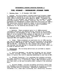
Figure 15 shows the z-factors calculated for reservoir fluid and injected fluid at different pressures. The change in reservoir fluid z-factor results from change in composition upon mixing with injected fluid with time. Also, Table 4 summarizes the difference between z-factor of the injected and reservoir fluids at different pressures. The injected fluid is mainly methane, while the produced gas is a mixture of methane and heavier hydrocarbon components contained in the reservoir fluid. It is clear from Figure 15 that compressibility factor of the injected gas is higher than that for the reservoir fluid at all cycles. Remembering that in the absence of an active aquifer, reservoir volume is constant during I/W cycles and reservoir behaves as a volumetric tank, higher z-factor results in the increase in reservoir pressure at the end of each I/W cycle. However, at successive I/W cycles, composition of reservoir fluid approaches that of the injected gas stream as a result of continual mixing. Theoretically, it is expected that composition of the reservoir fluid will be equal to the injected fluid after infinite I/W cycle, provided complete mixing occurs in the reservoir. Under these conditions, the difference between

500

2200

(3)

γg gas specific gravity; Tpc pseudo critical temperature; ppc pseudo critical pressure.

2600

ΔP/Cycle (psia)

Pressure at the start of cycle (psia)

(2) vL is liquid phase specific volume, and can be calculated by reliable correlations like that developed by Eslami and Azin [17, 18]; vg is the gas phase specific volume, and can be calculated either by correlations or by equations of state (EOS); x is the mole fraction of liquid in reservoir, which can be calculated by a flash calculation at specified P and T. If the liquid hydrocarbon volume of reservoir at the end of depletion and during I/W cycles is small compared to reservoir gas volume, as it is in this case, the composition of gas remaining in the reservoir can be assumed as reservoir fluid at the end of each I/W cycle, and reservoir gas density (or specific volume) can be used to calculate compressibility factor of the reservoir fluid and study the changes in z-factor during successive cycles as a result of lean gas injection. This analysis was done on Model 5 where a weak aquifer was selected for analysis. The compressibility factor, z, was calculated for produced gas at each I/W cycle using DranchukAbu-Kassem correlation [19]. This correlation is applicable over the following ranges: 0.2 ≤ ppr ≤ 30 1.0 < Tpr < 3.0

T pc = 168 + 325 γ g − 12.5 γ2g

Reservoir fluid Injected fluid

0.900 0.895 0.890 0.885 Depletion pressure

0.880 0.875

Initial reservoir pressure

0.870 0.865 1000

1400

1800 2200 2600 Pressure (psia)

3000

Figure 15 Figure 14 Reservoir pressure and ΔP/Cycle in models 4, 5, 6, and 7.

z-factors for the reservoir fluid and injected fluid at different pressures.

3400

702

Oil & Gas Science and Technology – Rev. IFP, Vol. 63 (2008), No. 6

z-factors of injected and reservoir fluids become smaller, as indicated in Table 4, and rate of pressure rise decreases. Finally, reservoir composition becomes uniform, and reservoir pressure will stabilize. TABLE 4 Difference between z-factor of the injected and reservoir fluids at different pressures Pressure, psia

Reservoir fluid z-factor (Zres)

Injected fluid z-factor (Zinj)

Zres – Zinj

3133.0 1488.2 1755.9 1766.8 1778.6 1789.0 1800.9 1812.4 1823.6 1832.8 1843.3 1853.4 1863.1

0.8690 0.8770 0.8877 0.8877 0.8880 0.8885 0.8889 0.8892 0.8895 0.8897 0.8899 0.8900 0.8901

0.9208 0.9177 0.9110 0.9108 0.9106 0.9104 0.9102 0.9099 0.9098 0.9096 0.9094 0.9093 0.9091

0.05179 0.04077 0.02331 0.02322 0.02254 0.02190 0.02128 0.02076 0.02031 0.01994 0.01958 0.01927 0.01903

reservoir fluid results in an increase in reservoir pressure during successive I/W cycles. Theoretically, composition of reservoir fluid will be equal to injected fluid after infinite I/W cycles, provided complete mixing occurs in the reservoir. Under these conditions, the difference between z-factors of injected and reservoir fluids become smaller, and the rate of pressure rise decreases. Finally, the reservoir composition becomes uniform, and reservoir pressure will stabilize. ACKNOWLEDGEMENTS

CONCLUSIONS If the gas reservoir is depleted down to its ultimate recovery, it may contain less base gas than required by gas storage operations. Under these conditions, the withdrawal rate from reservoir may not meet the target rate in the high-consumption seasons. When reservoir is depleted down to a very low pressure and has insufficient base gas reserve, operator can start withdrawal at a lower target rate and let the reservoir take enough pressure before raising the target pressure. Alternatively, it can prolong the injection period in the first cycle in order to inject sufficient reserve into reservoir before starting withdrawal. When reservoir is fed with a higher volume of gas in the first cycle, the production rate of condensate is higher. This is economically advantageous in gas condensate reservoirs, as production of condensate is economically attractive. A model with the highest aquifer permeability has the highest pressure at the start of I/W cycles. This is due to pressure support by active aquifer. Also, the water level and water-gas ratio will be higher under similar conditions. The pressure rise in reservoir during I/W cycles is due to the act of encroached water and/or difference between z-factor of injecting and reservoir fluids. Even in the absence of encroaching aquifer, the difference between compressibility factor of the injected gas and

This research was supported financially by Persian Gulf University, contract number 2/1386. The authors appreciate Dr. A. Ghaemi and Mr. R. Foruzanfar from Tehran Energy Consultants, Dr. H. Hassanzadeh from National Iranian Oil Company, and Prof. M. Moshfeghian from John M. Campbell & Co. for their valuable comments and help in preparing this paper. REFERENCES 1 Katz D.L., Cornell D., Var J.H., Kobayashi R., Elenbaas J.L., Poettmann F.H., Weinaug Ch.F. (1959) Handbook of Natural Gas Engineering, 1st edition, McGraw-Hill. 2 Chabrelie M.F., Dussaud M., Bourjas D., Hugout B. (2007) Underground Gas Storage: Technological Innovations for Increased Efficiency, World Energy Council. 3 Bennion D.B., Thomas F.B., Ma T., Imer D. (2000) Detailed Protocol for the Screening and Selection of Gas Storage Reservoir, SPE 59738, presented at the SPE/CERI Gas Technology Symposium, 2-5 April, Calgary, Alberta, Canada. 4 Coats K.H. (1966) Some Technical and Economic Aspects of Underground Gas Storage, J. Petrol. Technol. 12, 1561-1566. 5 Mayfield J.F. (1981) Inventory Verification of Gas Storage Fields, J. Petrol. Technol. 9, 1730-1734. 6 Schlumberger (2004) Eclipse Reference Manual. 7 Peng D.Y., Robinson D.B. (1976) A new Two-Constant Equation of State, Ind. Eng. Chem. Fundam. 15, 59-64. 8 Gumrah F., Izgec Ö., Gokecesu U., Bagci S. (2005) Modelling of Underground Gas Storage in a Depleted Gas Field, Energ. Source. Part A 27, 913-920. 9 Bagci A.S., Oztuk E. (2007) Performance Prediction of Underground Gas Storage in Salt Caverns, Energ. Source. Part B 2, 155-165. 10 Khamehchi E., Rashidi F. (2006) Simulation of Underground Natural Gas Storage in Sarajeh Gas Field, Iran, SPE 106341, presented at the SPE technical Symposium of Saudi Arabia, 2123 May, Dhahran, Saudi Arabia. 11 Griffith H.D., Rinehart R.D. (1971) Early Planning for Gas Storage Pays off – A Case History of Kentucky’s Largest Gas Field, SPE 3434, presented at the 46th Annual Fall Meeting of SPE-AIME, October 3-6, New Orleans, USA. 12 Chierici G.L., Pizzi G., Gucci G.M. (1967) Water Drive Gas Reservoirs: Uncertainty in Reserves Evaluation from Past History, JPT, pp. 237-244. 13 Craft B.C., Hawkins M.F., Terry R.E. (1991) Applied Petroleum Reservoir Engineering, 2nd edition, Prentice-Hall.

R Azin et al. / Underground Gas Storage in a Partially Depleted Gas Reservoir

14 Hower T.L., Fugate M.W., Owens R.W. (1993) Improved Performance in Aquifer Gas Storage fields through reservoir management, SPE 26172, presented at the SPE Gas Technology Symposium, 28-30 June, Calgary, Alberta, Canada. 15 Xiao G., Zhimin D., Ping G., Yuhong D., Yu F., Tao L. (2006) Design and demonstration of Creating Underground Gas Storage in a Fractured Oil Depleted Carbonate Reservoir, SPE 102397, presented at the SPE Russian Oil and Gas Technical Conference and Exhibition, 3-6 October, Moscow, Russia. 16 Aminan K., Bannon A., Ameri S. (2006) Gas Storage in a Depleted Gas/Condensate Reservoir in the Appalachian Basin, SPE 104555, presented at the 2006 SPE Eastern Regional Meeting, 11-13 October, Canton, Ohio, USA.

703

17 Eslami H., Azin R. (2003) Corresponding-States Correlation for Compressed Liquid Densities, Fluid Phase Equilibr. 209, 245-254. 18 Eslami H., Azin R. (2004) Corresponding-States Correlation for Compressed Liquid Density of Mixtures, Fluid Phase Equilibr. 226, 103-107. 19 Dranchuk P.M., Abu-Kassem J.H. (1975) Calculation of zfactors for Natural Gases Using Equations-of-State, JCPT, July-September, pp. 34-36. 20 Standing M.B. (1977) Volumetric and Phase Behavior of Oil Field Hydrocarbon Systems, Society of Petroleum Engineers. Final manuscript received in March 2008 Published online in September 2008

Copyright © 2008 Institut français du pétrole Permission to make digital or hard copies of part or all of this work for personal or classroom use is granted without fee provided that copies are not made or distributed for profit or commercial advantage and that copies bear this notice and the full citation on the first page. Copyrights for components of this work owned by others than IFP must be honored. Abstracting with credit is permitted. To copy otherwise, to republish, to post on servers, or to redistribute to lists, requires prior specific permission and/or a fee: Request permission from Documentation, Institut français du pétrole, fax. +33 1 47 52 70 78, or [email protected].