World Academy of Science, Engineering and Technology International Journal of Mechanical, Aerospace, Industrial, Mechatronic and Manufacturing Engineering Vol:8, No:8, 2014

Robotic Arm Control with Neural Networks Using Genetic Algorithm Optimization Approach A. Pajaziti, H. Cana

International Science Index, Mechanical and Mechatronics Engineering Vol:8, No:8, 2014 waset.org/Publication/9999081

Abstract—In this paper, the structural genetic algorithm is used to optimize the neural network to control the joint movements of robotic arm. The robotic arm has also been modeled in 3D and simulated in real-time in MATLAB. It is found that Neural Networks provide a simple and effective way to control the robot tasks. Computer simulation examples are given to illustrate the significance of this method. By combining Genetic Algorithm optimization method and Neural Networks for the given robotic arm with 5 D.O.F. the obtained the results shown that the base joint movements overshooting time without controller was about 0.5 seconds, while with Neural Network controller (optimized with Genetic Algorithm) was about 0.2 seconds, and the population size of 150 gave best results.

Method of structural optimization with genetic algorithm is on the border between neural networks and fuzzy logic on the one hand and genetic algorithm on the other side [2]. Indeed, structural genetic algorithm introduces a completely new method of combining different soft computing techniques to each other. Combining two or more optimization techniques leads to achieving the advantages of one or both optimization methods. In our case, we combined GA optimization method and neural networks.

Keywords—Robotic Arm, Neural Network, Genetic Algorithm, Optimization.

I. INTRODUCTION

S

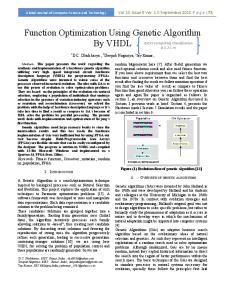
TRUCTURAL genetic algorithm was first introduced in the nineties, where the chromosomes are defined as the hierarchical structure. Nodes keep a higher level activation and operation of the genes, which are at a lower level. Inactivated genes provide additional information that the genetic algorithm can respond in a changing environment. Structural genetic algorithm as a structural optimizer is rapidly evolving and improving. In control applications there are two types optimizer's of particular importance: • Optimization of membership rules in fuzzy logic and • Optimizing the topology of neural networks. Fig. 1 shows how the structural genetic algorithm is used to optimize the neural network. Chromosome is broken up into control genes and genes connection [1]. Control bits are further divided into control bits of neural network layers and the control bits of individual neurons in the neural layers. If a single control bit logical value is 1, then a neural network layer and the corresponding neuron in layer exists, and vice versa, if the individual control bit is set to logic 0. The value of "x" means that the value (or logical 0 or 1) is not important. Connecting genes represent the values of the weights and thresholds of individual neurons this neuron is associated with pre-layer Neural Network (NN). Genetic Algorithm (GA) optimization of both structured genes is classic.

Fig. 1 Illustration of the structural genetic algorithm

In our case, vulnerable NN that can be "trapped" in a local minimum are eliminated by using the algorithm of the GA. If the function is non-linear, as shown in Fig. 2, the NN may be stuck in a local minimum, and from this it can be "solved" by GA.

A. Pajaziti is with the Department of Mechatronics, Faculty of Mechanical Engineering, University of Prishtina, Prishtina, 10000 Kosovo (phone: 38138-554-997; fax: 381-38-554-997; e-mail: [email protected]). H. Cana is a Master student with the Department of Mechatronics, Faculty of Mechanical Engineering, University of Prishtina, Prishtina, 10000 Kosovo (e-mail: [email protected]).

International Scholarly and Scientific Research & Innovation 8(8) 2014

Fig. 2 Local and global optimum

1431

scholar.waset.org/1999.8/9999081

World Academy of Science, Engineering and Technology International Journal of Mechanical, Aerospace, Industrial, Mechatronic and Manufacturing Engineering Vol:8, No:8, 2014

International Science Index, Mechanical and Mechatronics Engineering Vol:8, No:8, 2014 waset.org/Publication/9999081

In order to address the major shortcomings of neural networks which can be found in optimization methods has lead many scientists to use the GA approach. The idea is such that the weights of a neuron of neural networks can be optimized by the genetic algorithm, Fig. 3.

Fig. 4 Robotic Arm [12]

Fig. 3 Control of neural network weights

With this change, we lose self-learning NN and thus its positive features we gain the possibility of being trapped in a local minimum. As the GA is slower than the neural networks, we have lost a few at a time to solve optimization, but we are primarily interested in a better result. The computational complexity involved with the numerical solution of the kinematics problem, and the capability of NNs to approximate arbitrary functions, attracted many researchers to apply NNs to this problem [3]-[9]. Most of these works use known solution of the Forward Kinematics or Inverse Kinematics problem to generate input-output patterns for the NN training process [10]. In this paper, we proposed combined GA optimization method and neural networks for robotic arm control. The key attribute of neural networks is the ability to serve as a general nonlinear model [11]. It has been shown that any function of practicable interest can be approximated arbitrarily close with a NN having enough neurons, at least one hidden layer, and an appropriate set of weights. The high speed of computation and general modeling capability of neural networks are very attractive properties for nonlinear compensation problems, as robot control problems are. II. ROBOTIC SYSTEM WITH FIVE D.O.F Control optimization of the robotic arm with 5 D.O.F [10] (see Fig. 4) is carried out in MATLAB Simulink module using a virtual model based on the real model. In our case, results from system using no controller is compared to using NN optimized with GA. Our basic idea was to include neural networks in the model of the robot arm whose weights are changed (optimized) using GA. Because robot is controlled using Forward Kinematics, we introduced five NN modules, one for each robot joint in order to allow individual operation of joints so that they do not depend on each other. Each NN block takes one joint angle input which is the feedback error and gives one output which is the voltage to be fed into the motors.

International Scholarly and Scientific Research & Innovation 8(8) 2014

A. Robotic Arm System A typical closed-loop feedback system is used for controlling the robotic arm, Fig. 5. The system consists of two main blocks, the controller and plant. In our case the controller module has been replaced with NN blocks. Robotic arm mechanical system block contains sensors, which measure the current position of all five joints, and these values are fed back to be subtracted in order to get the error, which is then fed to NN to calculate the voltage value to produce motion using virtual motors in Simulink.

Fig. 5 Block diagram of robotic arm feedback system

B. 3D Robotic Arm Model Simulation The robotic arm in this paper has also been modeled in 3D using SolidWorks and then imported in MATLAB using SimMechanics Link which generates a basic block diagram of the model which represents only the geometrical aspect of the model which can be used for various analysis of the robotic arm, such as the usage of structural genetic algorithm to optimize the NN. The 3D model design and simulation of the arm has a number of advantages such performing analysis on PC which require high processing power and which can be completed faster than in microcontrollers and also these analyses are performed by quickly prototyping control systems using Simulink blocks.

1432

scholar.waset.org/1999.8/9999081

World Academy of Science, Engineering and Technology International Journal of Mechanical, Aerospace, Industrial, Mechatronic and Manufacturing Engineering Vol:8, No:8, 2014

International Science Index, Mechanical and Mechatronics Engineering Vol:8, No:8, 2014 waset.org/Publication/9999081

Fig. 6 3D virtual model of the robotic arm

III. THE INCLUSION OF A NEURAL NETWORK MODEL OF THE ROBOTIC ARM The neural network consists of one input neuron, ten neurons used in the hidden layer and one neuron in the output layer. Such a structure satisfied our requirements. In the event of an increase in the number of neurons in the hidden layer, this would lengthen the time simulation. It is known that the time required for the simulation by using the GA is longer. GA has served us to calculate the weights of neural networks and let us eliminate vulnerability of neural networks, because only this can be the bad choice of weights trapped in a local minimum. Fig. 7 shows structure of the neural network, where one can see the separation of the network into two levels.

Fig. 7 Appearance of neural networks separated by layers

Considering the fact that the robotic arm motors can only operate up to 180 degrees, the input and output of the NN are processed by limiting in and out values to a certain range. Input values are usually limited to -90 to 90 (degrees), while the output values are limited to -5 to 5 (volts), and this is done to avoid unnecessary values.

Fig. 8 Illustration of Neural Network - Layer 1

Figs. 8 and 9 show an image of the hidden layer weights (Layer 1) of neural network with ten neurons.

Fig. 9 Implementation of the Neural Network hidden layer weights in MATLAB Simulink - Layer 1

The second layer is similar to the first, except that in the hidden layer there are ten neurons (with weights IW{1,1}{110} which are fed as input in the second layer. Neural network weights (IW) initially are set to initial values which do not represent correct input-output relationship. After GA optimization is done, these weights are altered to optimized values along with bias. IV. SIMULATION RESULTS The work presented in this paper is based on the simulation of neural network control and genetic algorithm optimization. Simulations have been carried out under the MATLAB/Simulink environment. For the given robotic arm with 5 D.O.F we used five NN block for all five joints. In particular, we needed to carry out the movement of robotic arm with minimum overshoot and, consequently minimizing errors. The simulation was carried out under various datasets for neural network. Final input/output dataset was defined as: inputs = [-90 -80 -70 -60 -50 -40 -30 -20 -10 0 10 20 30 40 50 60 70 80 90]; outputs = [-5 -5 -5 -5 -5 -5 -5 -5 0 0 0 5 5 5 5 5 5 5 5]; The above input/output dataset represents the relationship between joint angle input values and motors’ voltage output

International Scholarly and Scientific Research & Innovation 8(8) 2014

1433

scholar.waset.org/1999.8/9999081

International Science Index, Mechanical and Mechatronics Engineering Vol:8, No:8, 2014 waset.org/Publication/9999081

World Academy of Science, Engineering and Technology International Journal of Mechanical, Aerospace, Industrial, Mechatronic and Manufacturing Engineering Vol:8, No:8, 2014

values which should result with an optimized curve representing this input/output relationship. As input reaches zero, so that voltage should decrease to avoid unnecessary overshoots. The initial values of the weights and biases for both the first and second layer are randomly generated based on NN input dataset. Number of weights which are needed for performing the simulation is 20, more specifically 10 weights for input and 10 weights for output. Also there are 10 biases for the hidden layer and one bias at the output layer. Values for these parameters are set after the genetic algorithm optimization is done. The number of generations used for optimization is 300 as higher numbers would lengthen the optimization time. In each iteration the mean square error is calculated. The optimization is performed using different numbers of population in order to get a good curve which is closest to the ideal dataset curve. Table I shows the best Fitness Value (FV) for three different population numbers through 300 iterations.

Fig. 11 Neural network after GA optimization

The neural network block with new weights and biases values replaces all five existing blocks in Simulink model in order to get results of joint movements with and without NN controller.

TABLE I GA OPTIMIZATION RESULTS WITH DIFFERENT POPULATION SIZES Population Iterations Weights for 2 Layers Best FV 50 300 20 0,690598 100 300 20 0,643956 150 300 20 0,677765

The lowest value of Best FV was given with population of 100 which resulted with a value of 0.643956. Fig. 10 shows the best fitness value falling from ~40 – 0.643956.

Fig. 12 Base joint movement without controller

Fig. 10 Best fitness value for population size 150

But considering the neural network optimization results with new weights and biases values, it turned out that the optimization with population size of 150 gave best results. Fig. 11 below represents the input/output relationship for the given dataset with blue line, green line represents this relationship before optimization (randomly generated weights values) and red line shows how the NN is about to behave after the optimization using GA. It results with a smooth curve which tries to follow the path of the input dataset curve.

International Scholarly and Scientific Research & Innovation 8(8) 2014

In order to get a clearer comparison between joint movements with and without controller, the value of motors’ stall torque has been increased. Fig. 12 shows the results of the base joint movements from 0 to 90 degrees. It shows some oscillations caused by overshooting when joint positions reach 90 degrees and settling time is about 0.5 seconds. Fig. 13 shows the base joint movement with NN controller (optimized with GA). The overshoot is much smaller in this case and settling time is about 0.2 seconds.

1434

scholar.waset.org/1999.8/9999081

International Science Index, Mechanical and Mechatronics Engineering Vol:8, No:8, 2014 waset.org/Publication/9999081

World Academy of Science, Engineering and Technology International Journal of Mechanical, Aerospace, Industrial, Mechatronic and Manufacturing Engineering Vol:8, No:8, 2014

Fig. 13 Base joint movement with NN controller

REFERENCES [1]

“Intelligent Control Techniques in Mechatronics - Genetic algorithm”, http://www.ro.feri.uni-mb.si/predmeti/int_reg/Predavanja/Eng/ 3.Genetic%20algorithm/_17.html [2] A. Pajaziti, I. Gojani, A. Shala, and P. Kopacek, “Optimization of Biped Gait Synthesis Using Fuzzy Neural Network Controller”, in DETC/CIE 2005-84191, September 2005. [3] R. K. Elsley, “A learning architecture for control based on backpropagation neural networks,” in International Conference on Neural Networks, vol. 2, pp. 587-594, IEEE, July 1988. [4] G. Josin, D. Charney, and D. White, “Robot control using neural networks,” in International Conference on Neural Networks, vol. 2, pp. 625-631, IEEE, July 1988. [5] S. Lee and R. M. Kil, “Robot kinematic control based on bi-directional mapping neural network,” in International Joint Conference on Neural Networks, vol. 3, pp. 327-335, 1990. [6] T. Yabuta and T. Yamada, “Possibility of neural networks controller for robot manipulators,” in International Conference on Robotics and Automation, pp. 16861691, IEEE, May 1990. [7] J. M. Zurada, M. Kavari, and J. H. Lilly, “Robot kinematics modeling using multilayer feedforward neural networks,” in Artificial Neural Networks in Engineering, pp. 785-790, ASME Press, November 1992. [8] L. C. Rabelo and X. J. R. Avula, “Hierarchical neurocontroller architecture for robotic manipulation,” IEEE Control Systems Magazine, vol. 12, no. 2, pp. 3741, April 1992. [9] K. Liu and J. P. H. Steele, “A new artificial neural systems architecture and its application to robot control,” in Artificial Neural Networks in Engineering, pp. 505-510, ASME Press, November 1993. [10] K. Liu and J. P. H. Steele, “A new artificial neural systems architecture and its application to robot control,” in Artificial Neural Networks in Engineering, pp. 505-510, ASME Press, November 1993. [11] D. Mandelc, “Soft computing in non-linear regulation”, individual research project, FEECS, University of Maribor, 2006 [12] H. Cana, “Manual and Semi-Automatic Control of Robotic Arm”, Master Thesis, University of Prishtina, Kosovo, 2014.

International Scholarly and Scientific Research & Innovation 8(8) 2014

1435

scholar.waset.org/1999.8/9999081