Sensor Network Optimization Using a Genetic Algorithm Shiyuan Jin, Ming Zhou, Annie S. Wu School of EECS University of Central Florida Orlando, FL 32816

[email protected], [email protected], [email protected]

ABSTRACT In this paper, we propose an efficient method based on genetic algorithms (GAs) to solve a sensor network optimization problem. Long communication distances between sensors and a sink (or destination) in a sensor network can greatly drain the energy of sensors and reduce the lifetime of a network. By clustering a sensor network into a number of independent clusters using a GA, we can greatly minimize the total communication distance, thus prolonging the network lifetime. Simulation results show that our algorithm can quickly find a good solution. This approach is also applicable to multiple network topologies (uniform or non-uniform) or shortest distance optimization problems . Keyword: Genetic algorithm, clustering, network optimization, shortest distance.

1. INTRODUCTIONS Wireless sensor networks are developing quickly and have been widely used in both military and civillian applications such as target tracking, surveillance, and security management. Since a sensor is a small, lightweight, un-tethered, battery-powered device, it has limited energy. Therefore, energy consumption is a critical issue in sensor networks. We are interested in sensor networks in which a large number of sensors are deployed to achieve a given goal. All data obtained by member sensors must be transmitted to a sink or data collector. The longer the communication distance, the more energy will be consumed during transmission. It is estimated that to transmit a k-bit message across a distance of d, the energy consumed can be represented as follows: E(k,d)=Eelec* k + Eamp*k*d2

[1]

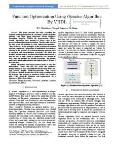
where Eelec is the radio energy dissipation and Eamp is transmit amplifier energy dissipation. Figure 1 is an example of direct transmission where each sensor transmits messages directly to the sink. Direct

Figure 1: An example of direct transmission transmission networks are very straightfoward to design but can be very power-consuming due to the long distances from sensors to the sink. Alternative designs that shorten or minimize the communication distances can extend network lifetimes. The use of clusters for transmitting data to a base station leverages the advantages of small transmit distances for most nodes, requiring only a few nodes to transmit far distances to the base station[1]. Clustering means to partition the network into a number of independent clusters, each of which has a cluster-head that collects data from all nodes within its cluster. These cluster-heads then compress the data and send it directly to the sink. Clustering can greatly reduce communication costs of most nodes because they only need to send data to the nearest cluster-head, rather than directly to a sink that may be further away. In this paper, we assume the sensor network is static. Sensors are deployed in a remote inhospitable environment and are far away from the sink which is usually positioned in a safe place. All nodes are assumed to have the capabilities of a cluster-head and the ability to adjust their transmission power based on transmission distance. Each sensor’s position can be precisely measured by GPS (Global Position System) devices. Clustering a network to minimize the total distance is an NP-hard[2] problem. For a given network topology, it is difficult to find the optimal number of cluster-heads and

their locations. Consider a 100-node example, to perform an exhausted search of all possible solutions requires 1

c

100

2

100

100

+ c100 + ... + c100 = 2

−1

different combination which is far too large to be handled by existing computer resources. A genetic algorithm is an efficient search algorithm that mimics the adaptive evolution process of natural systems. It has been successfully applied to many NP-hard problems such as multi-processor task scheduling, optimization, and traveling salesman problems. We propose to apply a GA to the problem of minimizing the total communication distance in a sensor network to efficiently reduce energy consumption and maximize the lifetime of the network.

2. RELATED WORK

All of the above algorithms assume a fixed number of clusters. We would like to solve a much harder problem where we do not know the number of clusters in advance. Our approach uses a GA to determine both the number and location of the cluster-heads that minimizes the communication distance in a sensor network.

3. PROPOSED GA SOLUTION We would like to use a GA to optimize the number of clusters and sensor connections for an arbitrary network. Once cluster-heads are selected, each regular node connects to its nearest cluster-head. Each node in a network is either a cluster-head or a “member“ of a cluster-head. Each regular node can only belong to one cluster-head. Each cluster-head collects data from all sensors within its cluster and each head directly sends the collected data to the sink. Figure 2 shows an example of clustering.

This work is motivated by Heinzelman et al’s paper[1] “Energy-Efficient Communication Protocol for Wireless Micro-sensor Networks” which describes a clusteringbased protocol called LEACH. They compare the performance of LEACH with direct communication and MTE. They use a pre-determined optimal number of clusters (5% of the total number of nodes) in their simulations. Heinzelman et al [3] determine that the optimal number of clusters for a 100-node network to be 3-5 by using a computation and communication energy model; however, determining the optimal number of cluster-heads depends on several factors such as sensor densities, the position of a sink, etc. Tillett et al[4] propose the PSO (Particle Swarm Optimization) approach to divide a sensor node field into groups of equal sized groups of nodes. PSO is an evolutionary programming technique that mimics the interaction of ants or termites to find a good solution. Although partitioning into equal sized clusters balances the energy consumption of cluster heads, this method is not applicable to some networks where nodes are not evenly distributed. Ostrosky et al[5] address a somewhat different partitioning problem: Given n points in a large data set, partition this data set into k ( k is known) disjoint clusters so as to minimize the total distance between all points and the cluster-heads to which they belong. The authors use a polynomial-time approximation scheme to solve the problem . Agarwal, et al[6] present an approximation algorithm to solve a clustering problem called k-clustering. This method separates the nodes in a workspace into k clusters where cluster membership is determined by a distance metric. As with the method proposed by Ostrosky et al, kclustering assumes a fixed number of clusters for optimization.

Figure 2: Clustering example 3.1 Problem Representation Finding appropriate cluster-heads is critically important to minimizing the distance. We use binary representation in which each bit corresponds to one sensor or node. A “1“ means that corresponding sensor is a cluster-head; otherwise, it is a regular node. In the following example individual, s1 s2 s3 s4 s5 s6 s7 s8 s9 1

0 0

1

0

0 1 0

0

nodes s1, s4 and s7 are cluster-heads. The remaining nodes are regular nodes. The initial population consists of randomly generated individuals. GA is used to select cluster-heads. Each regular node uses a deterministic method to find its nearest cluster-head. 3.2 GA Operators Crossover and mutation provide exploration, compared with the exploitation provided by selection. The effectiveness of GA depends on the trade-off between

exploitation and exploration. Crossover: In this paper, we use one-point crossover. The crossover operation takes place between two consecutive individuals with probability specified by crossover rate. These two individuals exchange portions that are separated by the crossover point The following is an example of crossover: Indv1: 1 1 1 0 0 1 0 1 Indv2: 1 0 1 1 1 1 1 0 Crossover point After crossover, two offspring are created as below: Child1: 1 1 1 0 1 1 1 0 Child2: 1 0 1 1 0 1 0 1 If a regular node becomes a cluster-head after crossover, all other regular nodes should check if they are nearer to this new cluster-head. If so, they switch their membership to this new head. This new head is detached from its previous head. If a cluster-head becomes a regular node, all of its members must find new cluster-heads. Every node is either a cluster-head or a member of a clusterhead in the network. Mutation: The mutation operator is applied to each bit of an individual with a probability of mutation rate. When applied, a bit whose value is 0 is mutated into 1 and vice versa. An example of mutation is as follows. Indv: 1 1 1 1 1 1 0 Indv: 1 1 1 0 1 1 1 3.3 Selection

where D is the total distance of all nodes to the sink; Distancei is the sum of the distances from regular nodes to clusterheads plus the sum of the distances from all clusterheads to the sink; Hi is the number of clusterheads; N is the total number of nodes; and w is a predefined weight. Except for distancei and Hi, all other parameters are fixed values in a given topology. The shorter the distance, or the lower the number of clusterheads, the higher the fitness value of an individual is. Our GA tries to maximize the fitness value to find a good solution. The value of w (0≤w≤1) is application-dependent. It indicates which factor is more important to be considered: distance or the cost incurred by cluster-heads. At one extreme, if w=1, we optimize the network only based on the communication distance. If w=0, only the number of cluster heads is considered. 3.5 Scaling Window When fitness values are similar, it can be difficult for a GA to distinguish better individuals from slightly worse individuals. This reduces the selection pressure toward the better structures, and the search stagnates[7]. In order to increase the probability of selecting the better individuals, we scale the fitness value of each individual by subtracting the minimum fitness value in each generation. Thus, the new fitness value fit(i)=Fit(i)-Fitmin. Figure 3 is an example of before and after scaling.

proportional distribution

Fit(1)=1020 (32.80%)

fit(1)= 0 (0.00%)

Fit(2)=1040 (33.44%)

fit(2)=20 (40.0%)

Fit(3)=1050 (33.76%)

fit(3)=30 (60.0%)

The selection process chooses the candidate individuals based on their fitnesses from the population in the current generation. Proportional selection (or roulette wheel selection) is used in this algorithm. It is implemented by using a biased roulette wheel, where each individual is assigned a slot, the size of which is proportional to the fitness value. Those individuals with higher fitness values are more likely to be selected as the individuals of population in the next generation. Figure 3:Proportional distribution before and after scaling.

3.4 Fitness Evaluation The total transmission distance is the main factor we need to minimize. In addition, the number of cluster heads can factor into the function. Given the same distance, fewer cluster heads result in greater energy efficiency as cluster heads drain more power than non-cluster-heads. Thus, each individual is evaluated by the following combined fitness components: Fitness = w* (D-distancei ) + (1-w)* (N– Hi)

After scaling, individual 3 has a higher probability to be selected as a candidate individual of the next generation.

4. EXPERIMENTAL RESULTS In our experiment, we randomly generate 100 nodes in a simulated 2-D environment and use two different sink positions (0,0) and (200,200). The following GA parameter settings are used throughout the experiments:

Population size: 80 Selection type: Proportional selection Crossover rate: 0.70 Crossover type: one-point Mutation rate: 0.006 Generation size: 800

Figure 5 shows an example output when the sink is located at (200,200) and w is set 0.8. Figure 6 shows an example output when w is set to 0, i.e. the number of cluster-heads is only considered in our fitness function. Although this is not realistic in our problem, it verifies the effectiveness of our algorithm because, as expected, the optimal number of heads is 1.

4.1 Clustering Results Figure 4 shows an example clustering result when the sink is located at (0,0), the upper left corner, and w is set 1.0; that is, we only consider the distance in our fitness function.

Figure 6: Clustering result with w = 0.

4.2 Changes of Fitness, Distance and Head over Generations Figure 4: Clustering result with sink at (0,0)

Figure 5: Clustering result with sink at (200,200)

Figures 7, 8, and 9 reflect the changes in the maximum fitness, the minimum distance and the number of heads, respectively, for an example run.

Figure 7: Maximum fitness over generations

(4) In a densely-deployed region, a middle node is generally elected as cluster-head. Figure 4 and figure 5 clearly show this. (5) No two cluster-heads are near to each other. The GA is likely to merge two nearby cluster-heads into one head to eliminate essentially duplicated communication distances. 4.3 Scalability

Figure 8: Minimum distances over generations

It is common to deploy hundreds of nodes in a sensor network if sensors are low in cost. As a result, it is very important to test the scalability of this algorithm, i.e., we want to test this when the number of nodes increases. We increase the number of nodes from 100, 200, to 400. Table 1 illustrates some initial test results when the sink is at (0,0). Table 1: Test Results of Three Problem Size Node Size

Figure 9: Cluster-head changes over generations Experimental results show that our algorithm is efficient and adaptive to multiple network topologies. (1) This approach can quickly find solutions. For a 100node problem, a good solution can be achieved after only 120 generations. Experiments indicate that the scaling window plays an important role in the quality of the solution found. (2) When a single node is near to the sink , that node itself becomes a cluster-head and sends data directly to the sink. Experiments also show that nodes near to the sink are more likely become cluster-heads than those far away. (3) More cluster-heads are needed when a sink is close to the center of a network than when it is located at a network corner. This observation is expected because when the sink is at the center, all regular nodes are located around the sink. As a result, cluster-heads tend to be distributed around the sink.

Population

Converge after generation

Head Distance (%) decreased

100

80

105

10.0%

76.85%

200

160

120

10.0%

81.20%

400

300

145

11.2%

82.20%

As the number of nodes doubles, it is necessary to double the population size to maintain comparable performance. The number of cluster-heads is about 10.0% of the total number of nodes. This percentage may vary if nodes are unevenly distributed. On average, distance is reduced by 80% as compared with the distance of direct transmission. This percentage increases slightly as node count increases because the larger the number of nodes and denser node distribution results in more efficient cluster optimization. As expected, in an application where nodes are densely distributed, reducing the number of heads tends to increase the solution quality significantly.

5. CONCLUSIONS AND FUTURE WORK In this paper, we propose a GA-based method to minimize communication distance in sensor networks via clustering. Our algorithm begins by randomly selecting nodes in a network to be cluster-heads. By adjusting cluster-heads based on fitness function, our algorithm is able to find an appropriate number of cluster-heads and their locations. Simulation results show that our approach is an efficient and effective method for solving this problem. First, it is able to quickly find good solutions. Second, this algorithm is applicable to both uniform and non-uniform network topologies. Our future work will focus on the comparison of our algorithm with others such as simulated annealing, Tabu search or other mathematical methods in terms of quality

and time-complexity. In addition, this network optimization problem can also be extended to a hierarchical structure where a cluster-head can have a super cluster-head which sends data directly to the sink. We believe this method can be scalable to larger problems and we plan to perform comprehensive tests to understand the impact of GA parameters. Applications of this approach can also be extended to other areas such as shortest distance optimization or base station construction where it is a challenging issue to determine the minimum number of base stations required to meet optimal radio transmission coverage while minimizing overall construction costs.

REFERENCES [1] W. R. Heinzelman, A. Chandrakasan, and H. Balakrishnan. Energy-Efficient Communication Protocol for Wireless Micro-sensor Networks. In Proceedings of the Hawaii International Conference on System Science, Maui, Hawaii,2000. [2]

P. Pardalos and H. Wolkowicz. Quadratic Assignments and Related Problems, DIMACS Series in Discrete Mathematics and Theoretical Computer Science, Vol. 16,1994.

[3] W. R. Heinzelman, A.P. Chandrakasan. An Application-Specific Protocol Architecture for Wireless Micro-sensor Network. IEEE Transactions on Wireless Communications, Vol. 1, No. 4, 2002. [4] J. Tillett, R. Rao, F. Sahin, and T.M. Rao. Clusterhead Identification in Ad hoc Sensor Networks Using Particle Swarm Optimization. In Proceedings of the IEEE International Conference on Personal Wireless Communication, 2002. [5] R. Ostrosky and Y. Rabani. Polynomial-Time Approxiamation Schemes for Geometric Min-Sum Median Clustering. Journal of the ACM, Vol. 49, No. 2, 2002, pp 139-156. [6] P. K. Agarwal, C. M. Procopiuc. Exact and approximation algorithms for clustering. In Proceedings of the Ninth Annual ACM-SIAM Symposium on Discrete Algorithms,1998. [7] J. J. Grefenstette. Optimization of Control Parameters for Genetic Algorithms. IEEE Transactions on Systems, Man and Cybernetics. Vol. SMC-16, No.1 January/February,1986.