2

Propositional Logic

In propositional logic, as the name suggests, propositions are connected by logical operators. The statement “the street is wet” is a proposition, as is “it is raining”. These two propositions can be connected to form the new proposition if it is raining the street is wet.

Written more formally it is raining ⇒ the street is wet.

This notation has the advantage that the elemental propositions appear again in unaltered form. So that we can work with propositional logic precisely, we will begin with a definition of the set of all propositional logic formulas.

2.1

Syntax

Definition 2.1 Let Op = {¬, ∧, ∨, ⇒, ⇔ , ( , )} be the set of logical operators and Σ a set of symbols. The sets Op, Σ and {t, f } are pairwise disjoint. Σ is called the signature and its elements are the proposition variables. The set of propositional logic formulas is now recursively defined: • t and f are (atomic) formulas. • All proposition variables, that is all elements from Σ , are (atomic) formulas. • If A and B are formulas, then ¬A, (A), A ∧ B, A ∨ B, A ⇒ B, A ⇔ B are also formulas. This elegant recursive definition of the set of all formulas allows us to generate infinitely many formulas. For example, given Σ = {A, B, C}, A ∧ B,

A ∧ B ∧ C,

A ∧ A ∧ A,

C ∧ B ∨ A,

(¬A ∧ B) ⇒ (¬C ∨ A)

are formulas. (((A)) ∨ B) is also a syntactically correct formula. W. Ertel, Introduction to Artificial Intelligence, Undergraduate Topics in Computer Science, DOI 10.1007/978-0-85729-299-5_2, © Springer-Verlag London Limited 2011

15

16

2

Propositional Logic

Definition 2.2 We read the symbols and operators in the following way: t: f: ¬A: A ∧ B: A ∨ B: A ⇒ B: A ⇔ B:

“true” “false” “not A” “A and B” “A or B” “if A then B” “A if and only if B”

(negation) (conjunction) (disjunction) (implication (also called material implication)) (equivalence)

The formulas defined in this way are so far purely syntactic constructions without meaning. We are still missing the semantics.

2.2

Semantics

In propositional logic there are two truth values: t for “true” and f for “false”. We begin with an example and ask ourselves whether the formula A ∧ B is true. The answer is: it depends on whether the variables A and B are true. For example, if A stands for “It is raining today” and B for “It is cold today” and these are both true, then A ∧ B is true. If, however, B represents “It is hot today” (and this is false), then A ∧ B is false. We must obviously assign truth values that reflect the state of the world to proposition variables. Therefore we define

Definition 2.3 A mapping I : Σ → {w, f }, which assigns a truth value to every proposition variable, is called an interpretation.

Because every proposition variable can take on two truth values, every propositional logic formula with n different variables has 2n different interpretations. We define the truth values for the basic operations by showing all possible interpretations in a truth table (see Table 2.1 on page 17). The empty formula is true for all interpretations. In order to determine the truth value for complex formulas, we must also define the order of operations for logical operators. If expressions are parenthesized, the term in the parentheses is evaluated

2.2

Semantics

Table 2.1 Definition of the logical operators by truth table

17 A

B

(A)

¬A

A∧B

A∨B

A⇒B

A⇔B

t

t

t

f

t

t

t

t

t

f

t

f

f

t

f

f

f

t

f

t

f

t

t

f

f

f

f

t

f

f

t

t

first. For unparenthesized formulas, the priorities are ordered as follows, beginning with the strongest binding: ¬, ∧, ∨, ⇒, ⇔ . To clearly differentiate between the equivalence of formulas and syntactic equivalence, we define

Definition 2.4 Two formulas F and G are called semantically equivalent if they take on the same truth value for all interpretations. We write F ≡ G.

Semantic equivalence serves above all to be able to use the meta-language, that is, natural language, to talk about the object language, namely logic. The statement “A ≡ B” conveys that the two formulas A and B are semantically equivalent. The statement “A ⇔ B” on the other hand is a syntactic object of the formal language of propositional logic. According to how many interpretations in which a formula is true, we can divide formulas into the following classes:

Definition 2.5 A formula is called • Satisfiable if it is true for at least one interpretation. • Logically valid or simply valid if it is true for all interpretations. True formulas are also called tautologies. • Unsatisfiable if it is not true for any interpretation. Every interpretation that satisfies a formula is called a model of the formula.

Clearly the negation of every generally valid formula is unsatisfiable. The negation of a satisfiable, but not generally valid formula F is satisfiable. We are now able to create truth tables for complex formulas to ascertain their truth values. We put this into action immediately using equivalences of formulas which are important in practice.

18

2

Propositional Logic

Theorem 2.1 The operations ∧, ∨ are commutative and associative, and the following equivalences are generally valid: ¬A ∨ B A⇒B (A ⇒ B) ∧ (B ⇒ A) ¬(A ∧ B) ¬(A ∨ B) A ∨ (B ∧ C) A ∧ (B ∨ C) A ∨ ¬A A ∧ ¬A A∨f A∨w A∧f A∧w

⇔ ⇔ ⇔ ⇔ ⇔ ⇔ ⇔ ⇔ ⇔ ⇔ ⇔ ⇔ ⇔

A⇒B ¬B ⇒ ¬A (A ⇔ B) ¬A ∨ ¬B ¬A ∧ ¬B (A ∨ B) ∧ (A ∨ C) (A ∧ B) ∨ (A ∧ C) w f A w f A

(implication) (contraposition) (equivalence) (De Morgan’s law) (distributive law) (tautology) (contradiction)

Proof To show the first equivalence, we calculate the truth table for ¬A ∨ B and A ⇒ B and see that the truth values for both formulas are the same for all interpretations. The formulas are therefore equivalent, and thus all the values of the last column are “t”s. A t t f f

B t f t f

¬A f f t t

¬A ∨ B t f t t

A⇒B t f t t

(¬A ∨ B) ⇔ (A ⇒ B) t t t t

The proofs for the other equivalences are similar and are recommended as exercises for the reader (Exercise 2.2 on page 29). 

2.3

Proof Systems

In AI we are interested in taking existing knowledge and from that deriving new knowledge or answering questions. In propositional logic this means showing that a knowledge base KB—that is, a (possibly extensive) propositional logic formula— a formula Q1 follows. Thus, we first define the term “entailment”.

1 Here

Q stands for query.

2.3

Proof Systems

19

Definition 2.6 A formula KB entails a formula Q (or Q follows from KB) if every model of KB is also a model of Q. We write KB | Q. In other words, in every interpretation in which KB is true, Q is also true. More succinctly, whenever KB is true, Q is also true. Because, for the concept of entailment, interpretations of variables are brought in, we are dealing with a semantic concept. Every formula that is not valid chooses so to speak a subset of the set of all interpretations as its model. Tautologies such as A ∨ ¬A, for example, do not restrict the number of satisfying interpretations because their proposition is empty. The empty formula is therefore true in all interpretations. For every tautology T then ∅ | T . Intuitively this means that tautologies are always true, without restriction of the interpretations by a formula. For short we write | T . Now we show an important connection between the semantic concept of entailment and syntactic implication.

Theorem 2.2 (Deduktionstheorem) A | B if and only if | A ⇒ B.

Proof Observe the truth table for implication: A t t f f

B t f t f

A⇒B t f t t

An arbitrary implication A ⇒ B is clearly always true except with the interpretation A → t, B → f . Assume that A | B holds. This means that for every interpretation that makes A true, B is also true. The critical second row of the truth table does not even apply in that case. Therefore A ⇒ B is true, which means that A ⇒ B is a tautology. Thus one direction of the statement has been shown. Now assume that A ⇒ B holds. Thus the critical second row of the truth table is also locked out. Every model of A is then also a model of B. Then A | B holds.  If we wish to show that KB entails Q, we can also demonstrate by means of the truth table method that KB ⇒ Q is a tautology. Thus we have our first proof system for propositional logic, which is easily automated. The disadvantage of this method is the very long computation time in the worst case. Specifically, in the worst case with n proposition variables, for all 2n interpretations of the variables the formula KB ⇒ Q must be evaluated. The computation time grows therefore exponentially

20

2

Propositional Logic

with the number of variables. Therefore this process is unusable for large variable counts, at least in the worst case. If a formula KB entails a formula Q, then by the deduction theorem KB ⇒ Q is a tautology. Therefore the negation ¬(KB ⇒ Q) is unsatisfiable. We have ¬(KB ⇒ Q) ≡ ¬(¬KB ∨ Q) ≡ KB ∧ ¬Q. Therefore KB ∧ ¬Q is also satisfiable. We formulate this simple, but important consequence of the deduction theorem as a theorem. Theorem 2.3 (Proof by contradiction) KB | Q if and only if KB ∧ ¬Q is unsatisfiable. To show that the query Q follows from the knowledge base KB, we can also add the negated query ¬Q to the knowledge base and derive a contradiction. Because of the equivalence A ∧ ¬A ⇔ f from Theorem 2.1 on page 18 we know that a contradiction is unsatisfiable. Therefore, Q has been proved. This procedure, which is frequently used in mathematics, is also used in various automatic proof calculi such as the resolution calculus and in the processing of PROLOG programs. One way of avoiding having to test all interpretations with the truth table method is the syntactic manipulation of the formulas KB and Q by application of inference rules with the goal of greatly simplifying them, such that in the end we can instantly see that KB | Q. We call this syntactic process derivation and write KB  Q. Such syntactic proof systems are called calculi. To ensure that a calculus does not generate errors, we define two fundamental properties of calculi. Definition 2.7 A calculus is called sound if every derived proposition follows semantically. That is, if it holds for formulas KB and Q that if

KB  Q

then KB | Q.

A calculus is called complete if all semantic consequences can be derived. That is, for formulas KB and Q the following it holds: if

KB | Q

then KB  Q.

The soundness of a calculus ensures that all derived formulas are in fact semantic consequences of the knowledge base. The calculus does not produce any “false consequences”. The completeness of a calculus, on the other hand, ensures that the calculus does not overlook anything. A complete calculus always finds a proof if the formula to be proved follows from the knowledge base. If a calculus is sound

2.3

Proof Systems

KB

21

Mod(KB)

| entailment

Mod(Q)

syntactic level (formula)

interpretation

Q

interpretation

 derivation

semantic level (interpretation)

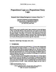
Fig. 2.1 Syntactic derivation and semantic entailment. Mod(X) represents the set of models of a formula X

and complete, then syntactic derivation and semantic entailment are two equivalent relations (see Fig. 2.1). To keep automatic proof systems as simple as possible, these are usually made to operate on formulas in conjunctive normal form.

Definition 2.8 A formula is in conjunctive normal form (CNF) if and only if it consists of a conjunction K1 ∧ K2 ∧ · · · ∧ Km of clauses. A clause Ki consists of a disjunction (Li1 ∨ Li2 ∨ · · · ∨ Lini ) of literals. Finally, a literal is a variable (positive literal) or a negated variable (negative literal).

The formula (A ∨ B ∨ ¬C) ∧ (A ∨ B) ∧ (¬B ∨ ¬C) is in conjunctive normal form. The conjunctive normal form does not place a restriction on the set of formulas because:

Theorem 2.4 Every propositional logic formula can be transformed into an equivalent conjunctive normal form.

22

2

Propositional Logic

Example 2.1 We put A ∨ B ⇒ C ∧ D into conjunctive normal form by using the equivalences from Theorem 2.1 on page 18: A ∨ B ⇒C ∧D ≡ ¬(A ∨ B) ∨ (C ∧ D) (implication) ≡ (¬A ∧ ¬B) ∨ (C ∧ D) (de Morgan) ≡ (¬A ∨ (C ∧ D)) ∧ (¬B ∨ (C ∧ D)) (distributive law) ≡ ((¬A ∨ C) ∧ (¬A ∨ D)) ∧ ((¬B ∨ C) ∧ (¬B ∨ D)) (distributive law) (associative law) ≡ (¬A ∨ C) ∧ (¬A ∨ D) ∧ (¬B ∨ C) ∧ (¬B ∨ D) We are now only missing a calculus for syntactic proof of propositional logic formulas. We start with the modus ponens, a simple, intuitive rule of inference, which, from the validity of A and A ⇒ B, allows the derivation of B. We write this formally as A,

A⇒B . B

This notation means that we can derive the formula(s) below the line from the comma-separated formulas above the line. Modus ponens as a rule by itself, while sound, is not complete. If we add additional rules we can create a complete calculus, which, however, we do not wish to consider here. Instead we will investigate the resolution rule A ∨ B, ¬B ∨ C A∨C

(2.1)

as an alternative. The derived clause is called resolvent. Through a simple transformation we obtain the equivalent form A ∨ B, B ⇒ C . A∨C If we set A to f , we see that the resolution rule is a generalization of the modus ponens. The resolution rule is equally usable if C is missing or if A and C are missing. In the latter case the empty clause can be derived from the contradiction B ∧ ¬B (Exercise 2.7 on page 30).

2.4

Resolution

We now generalize the resolution rule again by allowing clauses with an arbitrary number of literals. With the literals A1 , . . . , Am , B, C1 , . . . , Cn the general resolution rule reads (A1 ∨ · · · ∨ Am ∨ B), (¬B ∨ C1 ∨ · · · ∨ Cn ) . (A1 ∨ · · · ∨ Am ∨ C1 ∨ · · · ∨ Cn )

(2.2)

2.4

Resolution

23

We call the literals B and ¬B complementary. The resolution rule deletes a pair of complementary literals from the two clauses and combines the rest of the literals into a new clause. To prove that from a knowledge base KB, a query Q follows, we carry out a proof by contradiction. Following Theorem 2.3 on page 20 we must show that a contradiction can be derived from KB ∧ ¬Q. In formulas in conjunctive normal form, a contradiction appears in the form of two clauses (A) and (¬A), which lead to the empty clause as their resolvent. The following theorem ensures us that this process really works as desired. For the calculus to be complete, we need a small addition, as shown by the following example. Let the formula (A ∨ A) be given as our knowledge base. To show by the resolution rule that from there we can derive (A ∧ A), we must show that the empty clause can be derived from (A ∨ A) ∧ (¬A ∨ ¬A). With the resolution rule alone, this is impossible. With factorization, which allows deletion of copies of literals from clauses, this problem is eliminated. In the example, a double application of factorization leads to (A) ∧ (¬A), and a resolution step to the empty clause.

Theorem 2.5 The resolution calculus for the proof of unsatisfiability of formulas in conjunctive normal form is sound and complete.

Because it is the job of the resolution calculus to derive a contradiction from KB ∧ ¬Q, it is very important that the knowledge base KB is consistent:

Definition 2.9 A formula KB is called consistent if it is impossible to derive from it a contradiction, that is, a formula of the form φ ∧ ¬φ.

Otherwise anything can be derived from KB (see Exercise 2.8 on page 30). This is true not only of resolution, but also for many other calculi. Of the calculi for automated deduction, resolution plays an exceptional role. Thus we wish to work a bit more closely with it. In contrast to other calculi, resolution has only two inference rules, and it works with formulas in conjunctive normal form. This makes its implementation simpler. A further advantage compared to many calculi lies in its reduction in the number of possibilities for the application of inference rules in every step of the proof, whereby the search space is reduced and computation time decreased. As an example, we start with a simple logic puzzle that allows the important steps of a resolution proof to be shown. Example 2.2 Logic puzzle number 7, entitled A charming English family, from the German book [Ber89] reads (translated to English):

24

2 Propositional Logic Despite studying English for seven long years with brilliant success, I must admit that when I hear English people speaking English I’m totally perplexed. Recently, moved by noble feelings, I picked up three hitchhikers, a father, mother, and daughter, who I quickly realized were English and only spoke English. At each of the sentences that follow I wavered between two possible interpretations. They told me the following (the second possible meaning is in parentheses): The father: “We are going to Spain (we are from Newcastle).” The mother: “We are not going to Spain and are from Newcastle (we stopped in Paris and are not going to Spain).” The daughter: “We are not from Newcastle (we stopped in Paris).” What about this charming English family?

To solve this kind of problem we proceed in three steps: formalization, transformation into normal form, and proof. In many cases formalization is by far the most difficult step because it is easy to make mistakes or forget small details. (Thus practical exercise is very important. See Exercises 2.9–2.11.) Here we use the variables S for “We are going to Spain”, N for “We are from Newcastle”, and P for “We stopped in Paris” and obtain as a formalization of the three propositions of father, mother, and daughter (S ∨ N ) ∧ [(¬S ∧ N ) ∨ (P ∧ ¬S)] ∧ (¬N ∨ P ). Factoring out ¬S in the middle sub-formula brings the formula into CNF in one step. Numbering the clauses with subscripted indices yields KB ≡ (S ∨ N )1 ∧ (¬S)2 ∧ (P ∨ N )3 ∧ (¬N ∨ P )4 . Now we begin the resolution proof, at first still without a query Q. An expression of the form “Res(m, n): clause k ” means that clause is obtained by resolution of clause m with clause n and is numbered k. Res(1, 2) :

(N )5

Res(3, 4) :

(P )6

Res(1, 4) :

(S ∨ P )7

We could have derived clause P also from Res(4, 5) or Res(2, 7). Every further resolution step would lead to the derivation of clauses that are already available. Because it does not allow the derivation of the empty clause, it has therefore been shown that the knowledge base is non-contradictory. So far we have derived N and P . To show that ¬S holds, we add the clause (S)8 to the set of clauses as a negated query. With the resolution step Res(2, 8) :

()9

the proof is complete. Thus ¬S ∧ N ∧ P holds. The “charming English family” evidently comes from Newcastle, stopped in Paris, but is not going to Spain. Example 2.3 Logic puzzle number 28 from [Ber89], entitled The High Jump, reads

2.5

Horn Clauses

25

Three girls practice high jump for their physical education final exam. The bar is set to 1.20 meters. “I bet”, says the first girl to the second, “that I will make it over if, and only if, you don’t”. If the second girl said the same to the third, who in turn said the same to the first, would it be possible for all three to win their bets?

We show through proof by resolution that not all three can win their bets. Formalization: The first girl’s jump succeeds: A, the second girl’s jump succeeds: B, the third girl’s jump succeeds: C.

First girl’s bet: (A ⇔ ¬B), second girl’s bet: (B ⇔ ¬C), third girl’s bet: (C ⇔ ¬A).

Claim: the three cannot all win their bets: Q ≡ ¬((A ⇔ ¬B) ∧ (B ⇔ ¬C) ∧ (C ⇔ ¬A)) It must now be shown by resolution that ¬Q is unsatisfiable. Transformation into CNF: First girl’s bet: (A ⇔ ¬B) ≡ (A ⇒ ¬B) ∧ (¬B ⇒ A) ≡ (¬A ∨ ¬B) ∧ (A ∨ B) The bets of the other two girls undergo analogous transformations, and we obtain the negated claim ¬Q ≡ (¬A ∨ ¬B)1 ∧ (A ∨ B)2 ∧ (¬B ∨ ¬C)3 ∧ (B ∨ C)4 ∧ (¬C ∨ ¬A)5 ∧ (C ∨ A)6 . From there we derive the empty clause using resolution: Res(1, 6) : Res(4, 7) : Res(2, 5) : Res(3, 9) : Res(8, 10) :

(C ∨ ¬B)7 (C)8 (B ∨ ¬C)9 (¬C)10 ()

Thus the claim has been proved.

2.5

Horn Clauses

A clause in conjunctive normal form contains positive and negative literals and can be represented in the form (¬A1 ∨ · · · ∨ ¬Am ∨ B1 ∨ · · · ∨ Bn )

26

2

Propositional Logic

with the variables A1 , . . . , Am and B1 , . . . , Bn . This clause can be transformed in two simple steps into the equivalent form A1 ∧ · · · ∧ Am ⇒ B1 ∨ · · · ∨ Bn . This implication contains the premise, a conjunction of variables and the conclusion, a disjunction of variables. For example, “If the weather is nice and there is snow on the ground, I will go skiing or I will work.” is a proposition of this form. The receiver of this message knows for certain that the sender is not going swimming. A significantly clearer statement would be “If the weather is nice and there is snow on the ground, I will go skiing.”. The receiver now knows definitively. Thus we call clauses with at most one positive literal definite clauses. These clauses have the advantage that they only allow one conclusion and are thus distinctly simpler to interpret. Many relations can be described by clauses of this type. We therefore define

Definition 2.10 Clauses with at most one positive literal of the form (¬A1 ∨ · · · ∨ ¬Am ∨ B)

or

(¬A1 ∨ · · · ∨ ¬Am )

or

B

or (equivalently) A1 ∧ · · · ∧ Am ⇒ B

or

A1 ∧ · · · ∧ Am ⇒ f

or B.

are named Horn clauses (after their inventor). A clause with a single positive literal is a fact. In clauses with negative and one positive literal, the positive literal is called the head.

To better understand the representation of Horn clauses, the reader may derive them from the definitions of the equivalences we have currently been using (Exercise 2.12 on page 30). Horn clauses are easier to handle not only in daily life, but also in formal reasoning, as we can see in the following example. Let the knowledge base consist of the following clauses (the “∧” binding the clauses is left out here and in the text that follows): (nice_weather)1 (snowfall)2 (snowfall ⇒ snow)3 (nice_weather ∧ snow ⇒ skiing)4

2.5

Horn Clauses

27

If we now want to know whether skiing holds, this can easily be derived. A slightly generalized modus ponens suffices here as an inference rule: A1 ∧ · · · ∧ Am ,

A1 ∧ · · · ∧ Am ⇒ B . B

The proof of “skiing” has the following form (MP(i1 , . . . , ik ) represents application of the modus ponens on clauses i1 to ik : MP(2, 3) : MP(1, 5, 4) :

(snow)5 (skiing)6 .

With modus ponens we obtain a complete calculus for formulas that consist of propositional logic Horn clauses. In the case of large knowledge bases, however, modus ponens can derive many unnecessary formulas if one begins with the wrong clauses. Therefore, in many cases it is better to use a calculus that starts with the query and works backward until the facts are reached. Such systems are designated backward chaining, in contrast to forward chaining systems, which start with facts and finally derive the query, as in the above example with the modus ponens. For backward chaining of Horn clauses, SLD resolution is used. SLD stands for “Selection rule driven linear resolution for definite clauses”. In the above example, augmented by the negated query (skiing ⇒ f ) (nice_weather)1 (snowfall)2 (snowfall ⇒ snow)3 (nice_weather ∧ snow ⇒ skiing)4 (skiing ⇒ f )5 we carry out SLD resolution beginning with the resolution steps that follow from this clause Res(5, 4) :

(nice_weather ∧ snow ⇒ f )6

Res(6, 1) :

(snow ⇒ f )7

Res(7, 3) :

(snowfall ⇒ f )8

Res(8, 2) :

()

and derive a contradiction with the empty clause. Here we can easily see “linear resolution”, which means that further processing is always done on the currently derived clause. This leads to a great reduction of the search space. Furthermore, the literals of the current clause are always processed in a fixed order (for example, from right to left) (“Selection rule driven”). The literals of the current clause are called

28

2 Propositional Logic

subgoal. The literals of the negated query are the goals. The inference rule for one step reads A1 ∧ · · · ∧ Am ⇒ B1 , B1 ∧ B2 ∧ · · · ∧ Bn ⇒ f . A1 ∧ · · · ∧ Am ∧ B2 ∧ · · · ∧ Bn ⇒ f Before application of the inference rule, B1 , B2 , . . . , Bn —the current subgoals— must be proved. After the application, B1 is replaced by the new subgoal A1 ∧ · · · ∧ Am . To show that B1 is true, we must now show that A1 ∧ · · · ∧ Am are true. This process continues until the list of subgoals of the current clauses (the so-called goal stack) is empty. With that, a contradiction has been found. If, for a subgoal ¬Bi , there is no clause with the complementary literal Bi as its clause head, the proof terminates and no contradiction can be found. The query is thus unprovable. SLD resolution plays an important role in practice because programs in the logic programming language PROLOG consist of predicate logic Horn clauses, and their processing is achieved by means of SLD resolution (see Exercise 2.13 on page 30, or Chap. 5).

2.6

Computability and Complexity

The truth table method, as the simplest semantic proof system for propositional logic, represents an algorithm that can determine every model of any formula in finite time. Thus the sets of unsatisfiable, satisfiable, and valid formulas are decidable. The computation time of the truth table method for satisfiability grows in the worst case exponentially with the number n of variables because the truth table has 2n rows. An optimization, the method of semantic trees, avoids looking at variables that do not occur in clauses, and thus saves computation time in many cases, but in the worst case it is likewise exponential. In resolution, in the worst case the number of derived clauses grows exponentially with the number of initial clauses. To decide between the two processes, we can therefore use the rule of thumb that in the case of many clauses with few variables, the truth table method is preferable, and in the case of few clauses with many variables, resolution will probably finish faster. The question remains: can proof in propositional logic go faster? Are there better algorithms? The answer: probably not. After all, S. Cook, the founder of complexity theory, has shown that the 3-SAT problem is NP-complete. 3-SAT is the set of all CNF formulas whose clauses have exactly three literals. Thus it is clear that there is probably (modulo the P/NP problem) no polynomial algorithm for 3-SAT, and thus probably not a general one either. For Horn clauses, however, there is an algorithm in which the computation time for testing satisfiability grows only linearly as the number of literals in the formula increases.

2.7 Applications and Limitations

2.7

29

Applications and Limitations

Theorem provers for propositional logic are part of the developer’s everyday toolset in digital technology. For example, the verification of digital circuits and the generation of test patterns for testing of microprocessors in fabrication are some of these tasks. Special proof systems that work with binary decision diagrams (BDD) () are also employed as a data structure for processing propositional logic formulas. In AI, propositional logic is employed in simple applications. For example, simple expert systems can certainly work with propositional logic. However, the variables must all be discrete, with only a few values, and there may not be any crossrelations between variables. Complex logical connections can be expressed much more elegantly using predicate logic. Probabilistic logic is a very interesting and current combination of propositional logic and probabilistic computation that allows modeling of uncertain knowledge. It is handled thoroughly in Chap. 7. Fuzzy logic, which allows infinitely many truth values, is also discussed in that chapter.

2.8

Exercises

➳ Exercise

2.1 Give a Backus–Naur form grammar for the syntax of propositional

logic. Exercise 2.2 Show that the following formulas are tautologies: (a) ¬(A ∧ B) ⇔ ¬A ∨ ¬B (b) A ⇒ B ⇔ ¬B ⇒ ¬A (c) ((A ⇒ B) ∧ (B ⇒ A)) ⇔ (A ⇔ B) (d) (A ∨ B) ∧ (¬B ∨ C) ⇒ (A ∨ C) Exercise 2.3 Transform the following formulas into conjunctive normal form: (a) A ⇔ B (b) A ∧ B ⇔ A ∨ B (c) A ∧ (A ⇒ B) ⇒ B Exercise 2.4 Check the following statements for satisfiability or validity. (a) (play_lottery ∧ six_right) ⇒ winner (b) (play_lottery ∧ six_right ∧ (six_right ⇒ win)) ⇒ win (c) ¬(¬gas_in_tank ∧ (gas_in_tank ∨ ¬car_starts) ⇒ ¬car_starts) ❄ ❄ Exercise

2.5 Using the programming language of your choice, program a theorem prover for propositional logic using the truth table method for formulas in conjunctive normal form. To avoid a costly syntax check of the formulas, you may represent clauses as lists or sets of literals, and the formulas as lists or sets of clauses. The program should indicate whether the formula is unsatisfiable, satisfiable, or true, and output the number of different interpretations and models.

30

2

Propositional Logic

Exercise 2.6 (a) Show that modus ponens is a valid inference rule by showing that A ∧ (A ⇒ B) | B. (b) Show that the resolution rule (2.1) is a valid inference rule. ❄ Exercise

2.7 Show by application of the resolution rule that, in conjunctive normal form, the empty clause is equivalent to the false statement.

❄ Exercise

2.8 Show that, with resolution, one can “derive” any arbitrary clause from a knowledge base that contains a contradiction. Exercise 2.9 Formalize the following logical functions with the logical operators and show that your formula is valid. Present the result in CNF. (a) The XOR operation (exclusive or) between two variables. (b) The statement at least two of the three variables A, B, C are true.

❄ Exercise

2.10 Solve the following case with the help of a resolution proof: “If the criminal had an accomplice, then he came in a car. The criminal had no accomplice and did not have the key, or he had the key and an accomplice. The criminal had the key. Did the criminal come in a car or not?” Exercise 2.11 Show by resolution that the formula from (a) Exercise 2.2(d) is a tautology. (b) Exercise 2.4(c) is unsatisfiable. Exercise 2.12 Prove the following equivalences, which are important for working with Horn clauses: (a) (¬A1 ∨ · · · ∨ ¬Am ∨ B) ≡ A1 ∧ · · · ∧ Am ⇒ B (b) (¬A1 ∨ · · · ∨ ¬Am ) ≡ A1 ∧ · · · ∧ Am ⇒ f (c) A ≡ w ⇒ A Exercise 2.13 Show by SLD resolution that the following Horn clause set is unsatisfiable. (A)1 (B)2 (C)3

➳ Exercise

(D)4 (E)5 (A ∧ B ∧ C ⇒ F )6

(A ∧ D ⇒ G)7 (C ∧ F ∧ E ⇒ H )8 (H ⇒ f )9

2.14 In Sect. 2.6 it says: “Thus it is clear that there is probably (modulo the P/NP problem) no polynomial algorithm for 3-SAT, and thus probably not a general one either.” Justify the “probably” in this sentence.

http://www.springer.com/978-0-85729-298-8