Propositional Modal Logic UC Berkeley, Philosophy 142, Spring 2016
1
John MacFarlane
Grammar
We add two new one-place sentential connectives to the language of propositional logic: ‘’ and ‘◊’. Grammatically these behave just like ‘¬’: if φ is a formula, then ðφñ and ð◊φñ are formulas. You can read ‘’ as “necessarily” and ‘◊’ as “possibly.” But modal logics, like other formal systems, can have many applications. Depending on the application, they might have many different meanings, for example: it is logically necessary that it could not have failed to happen that it must be the case that it is now settled that it is obligatory that it is provable that A believes that A knows that
◊ it is logically possible that it might have happened that it might be the case that it is still possible that it is permitted that it is not refutable that A regards it as an open possibility that for all A knows, it may be true that
Sometimes the letters ‘L’ and ‘M ’ are used instead of ‘’ and ‘◊’. Sometimes an operator for contingency is defined: Ïφ =d e f (◊φ ∧ ◊¬φ).
2 2.1
◊
Ï
Semantics Models
Our models for classical propositional logic were just assignments of truth values to the propositional constants—what is represented by the rows of a truth table. Models for modal logic must be more complex. A model for modal propositional logic is a quadruple 〈W , R, @,V 〉, where W is a nonempty set of objects (the worlds), R is a relation defined on W (the accessibility relation), @ is a member of W (the actual world of the model), and V is a function (the valuation that assigns a truth value to each pair of a propositional constant and a world. The triple 〈W , R, @〉 (without the valuation) is called a frame. So you can think of a model as consisting of a frame + a valuation. February 16, 2016
1
model
worlds accessibility relation actual world valuation
frame
2.2
Truth in a model for modal formulas
What are the worlds? In many standard applications of modal logic, you can think of the worlds as possible worlds—ways things could be, determinate down to the last detail. You can think of the valuation function as telling us which propositions would be true in which possible worlds, that is, which would be true if things were a certain way. The “actual world” @ represents the way things actually are (according to the model). There are a lot of controversies about how we should think of possible worlds, metaphysically speaking: whether we should think of them as concrete worlds or as abstract models or sets of sentences, for example.1 For the most part, we can ignore these controversies when we’re just doing logic. You can think of the accessibility relation as embodying a notion of relative possibility. The worlds that are accessible from a given world are those that are possible relative to it. If this seems too abstract, you can join Hughes and Cresswell in thinking of the worlds as seats, and the accessibility relation as the relation that holds between two seats if someone sitting in the first can see the person sitting in the second. Or think of the worlds as people and the accessibility relation as the relation of loving. When we’re considering the logics abstractly, without regard to their applications, it doesn’t really matter. 2.2
accessible
Truth in a model for modal formulas
We define truth in a model for modal formulas in terms of quantification over worlds. Possibility is understood as truth in some accessible world, and necessity as truth in all w φ’ means ‘φ is true in model M at world w’. All the action accessible worlds. Here ‘M is in the last two clauses:
w M φ
true in a model at a world
w • If φ is a propositional constant, 〈W φ iff V (φ, w) = True. ,R,@,V 〉 w w • 〈W ð¬φñ iff 2〈W φ. ,R,@,V 〉 ,R,@,V 〉 w w w φ and 〈W ψ. • 〈W ðφ ∧ ψñ iff 〈W ,R,@,V 〉 ,R,@,V 〉 ,R,@,V 〉 0
w w • 〈W ð◊φñ iff for some w 0 ∈ W such that Rw w 0 , 〈W φ. ,R,@,V 〉 ,R,@,V 〉 0
w w • 〈W ðφñ iff for every w 0 ∈ W such that Rw w 0 , 〈W φ. ,R,@,V 〉 ,R,@,V 〉
So far we have defined truth in a model at a world. We can define (plain) truth in a model in terms of this as follows:
true at a model
A formula φ is true in a model 〈W , R, @,V 〉 if @ φ. 〈W ,R,@,V 〉 That is, a formula is true at a model if it is true at the model’s “actual world.” We can now define the logical properties as usual in terms of truth at a model. A sentence is logically true if it is true in all models; an argument is valid if the conclusion is true in every model in which all the premises are true; and so on. If you want to get into this debate, I recommend starting with [5], then turning to [3], David Lewis’s magisterial defense of the concretist viewpoint. [4] collects many relevant papers. 1
February 16, 2016
2
logically true valid
2.3
The modal logic K
2.3
The modal logic K
If we define the logical properties this way and make no further restrictions on what counts as a model, we get the modal logic K. K is the weakest of the modal logics we’ll look at, and everything that is valid in K is valid in all the others. Here are some formulas that are logically true in K: (1)
K
a. (P ∧ Q) ⊃ (P ∧ Q) b. (P ∧ Q) ⊃ (P ∧ Q) c. ¬P ≡ ◊¬P d. ¬P ≡ ¬◊P
Can you see why they are true in all models? Think about (1a) and (1b) this way: if ‘P ∧ Q’ is true in all accessible worlds, then it must be that P is true in all those worlds, and Q is true in all those worlds. The converse also holds: if P is true in all accessible worlds, and so is Q, then ‘P ∧ Q’ is true in all accessible worlds. Do you see the resemblance between (1c) and (1d) and the quantifier-negation equivalences? What explains this resemblance? Here is a formula that is not logically true in K: (2)
P ⊃ P
Can you see why not? Here is an invalidating model:
@
w2
V P
@ False
w2 True
Here P is false in @, even though it is true at every world accessible from @. Exercise: 2.3.1 Find a K-model in which ‘P ⊃ ◊P ’ is false.
2.4
The modal logic D
If you add ‘φ ⊃ ◊φ’ as an axiom schema to K, you get a stronger logic D. (To say that D is stronger than K is to say that every argument valid in K is also valid in D, but there are some arguments that are valid in D but not in K.) D is stronger than K, there must be K-models that are not D-models. (For, if every K-model were a D-model, any argument that preserved truth in every K-model would preserve truth in every D-model.) In fact, D-models are K-models that meet an additional restriction: the accessibility relation must be serial. February 16, 2016
3
stronger
2.5
The modal logic T A relation R on W is serial iff ∀w ∈ W ∃w 0 ∈ W Rw w 0 .
serial
What this means, intuitively, is that there are no “dead ends”—no worlds that can’t “see” any worlds (including themselves). With dead ends ruled out, ‘P ⊃ ◊P ’ no longer has countermodels. What about (2)? The invalidating model we used before isn’t a D-model, because w2 is a dead end. Can you find a D-model that makes (2) false?) Note that on the deontic interpretation of the modal operators, where ‘’ means “it is obligatory that” and ‘◊’ means “it is permissible that,” ‘φ ⊃ ◊φ’ is the very plausible principle that whatever is obligatory is permissible. And in a deontic logic, we don’t want ‘φ ⊃ φ’, since what is obligatory doesn’t always happen. So D is a good logic for this interpretation. 2.5
The modal logic T
If you add ‘φ ⊃ φ’ as an axiom schema to D, you get a stronger logic T. A T-model is a K-model whose accessibility relation is reflexive. A relation R on W is reflexive iff ∀w ∈ W Rw w. That is, every world can see itself.
reflexive
Since every reflexive accessibility relation is serial, every T-model is a D-model. The converse does not hold: there are D-models that are not T-models. Hence, every argument that is valid in D is valid in T, but not every argument that is valid in T is valid in D. Exercise: 2.5.1 Find a T-model in which ‘P ⊃ P ’ is false. 2.5.2 Describe a D-model that is not a T-model.
2.6
The modal logic S4
If you add ‘φ ⊃ φ’ as an axiom schema to T, you get a stronger logic S4. An S4-model is a K-model whose accessibility relation is reflexive and transitive. A relation R on W is transitive iff ∀w0 , w1 , w2 ∈ W ((Rw0 w1 ∧ Rw1 w2 ) ⊃ Rw0 w2 ).
transitive
Theorems of S4 include ‘◊◊P ⊃ ◊P ’ and ‘◊◊P ⊃ ◊P ’. Exercise: 2.6.1 Find an S4-model in which ‘◊P ⊃ ◊P ’ is false. 2.6.2 Find an S4-model in which ‘◊P ⊃ P ’ is false.
February 16, 2016
4
2.7
The modal logic B
2.7
The modal logic B
If you add ‘φ ⊃ ◊φ’ as an axiom schema to T, you get a stronger logic B. (Note that neither B nor S4 is stronger than the other; there are logical truths of B that are not logical truths of S4, and vice versa.) A B-model is a K-model whose accessibility relation is reflexive and symmetric. A relation R on W is symmetric iff ∀w, w 0 ∈ W (Rw w 0 ≡ Rw 0 w).
symmetric
Exercise: 2.7.1 Find a B-model in which ‘◊P ⊃ ◊P ’ is false.
2.8
The modal logic S5
If you add ‘◊φ ⊃ ◊φ’ as an axiom schema to T, you get a stronger logic S5. S5 is stronger than both S4 and B. An S5-model is a K-model whose accessibility relation is reflexive, symmetric, and transitive. That is, it is an equivalence relation. An equivalence relation partitions the worlds into cells, where each world in a cell can see each other world in that cell (including itself). It is easy to see that if a formula can be falsified by an S5-model, it can be falsified by a universal S5-model—one in which every world is accessible from every other. (Just remove all the cells except the one containing the actual world, and you’ll have a universal S5-model that falsifies the same sentences.) So we get the same logic if we think of our models as just sets of worlds, and talk of necessity as truth in all worlds, forgetting about the accessibility relation. S5 is the most common modal logic used by philosophers. Exercise: 2.8.1 Find an S5-model in which ‘◊P ⊃ P ’ is false.
2.9
Summary
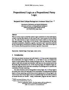
The relationships between these six modal systems are summarized in Table 1 and Fig. 1.
February 16, 2016
5
equivalence relation
2.9
Summary
Table 1: Summary of the main systems of propositional modal logic. Logic K D T S4 B S5
Restrictions on accessibility relation — serial reflexive reflexive, transitive reflexive, symmetric reflexive, symmetric, transitive
Characteristic axiom — φ ⊃ ◊φ φ ⊃ φ φ ⊃ φ φ ⊃ ◊φ ◊φ ⊃ ◊φ
S5 +symmetric +transitive S4
B
+transitive +symmetric T +reflexive D +serial K
Figure 1: Relations between the systems; arrows point to stronger systems.
February 16, 2016
6
3. Proofs
3
Proofs
By supplementing our existing proof system for propositional logic with a few rules for the modal operators, we can get new proof systems for T, S4, and S5. For all these systems, we’ll need some modal-negation equivalences. These are replacement rules, so they can go in either direction and work even in subformulas (just like the parallel quantifier-negation equivalences): Modal-negation equivalences (MNE) ¬◊φ ⇐⇒ ¬φ ¬φ ⇐⇒ ◊¬φ
MNE
We’ll also need rules for Elim and ◊ Intro:
Elim, ◊-Intro
φ ◊ Intro ◊φ
φ Elim φ
Finally, we need some way of introducing a ‘’. Obviously we can’t have the converse of Elim, since that would let us prove every instance of ðφ ≡ φñ, and our modal logic would be trivialized. We don’t want to argue: “Fido is lying down; so, it is necessary that Fido be lying down.” The trick is to allow ‘’ to be introduced only through a special kind of subproof. We will mark these subproofs with a small box to the left of the subproof line. (Some texts suggest putting a double line across the top of the subproof, or a box around the whole thing, to indicate that it is “sealed off” from the outside context, and you may want to do that.) If you have a modal subproof that ends with a formula φ, you can close off the subproof and write ðφñ on the next line, with justification “ Intro.”
2
.. . .. .
3
φ
4
φ
1
(1) Intro 1–3
What is special about modal subproofs is that there are strict restrictions on the use of premises from outside the subproofs. In a normal subproof, you can use any formula that occurs above the current position in a proof, and in the same subproof or a subproof containing it. For example,
February 16, 2016
7
3. Proofs
P
1 2
Q
hyp
3
P ∧Q
∧ Intro 1, 2
Q ⊃ (P ∧ Q)
4
(2)
⊃ Intro 2–3
In our modal subproofs, by contrast, this won’t be allowed: P
1 2
3 4 5
Q
hyp
P ∧Q
∧ Intro 1, 3 ⇐ ILLEGAL!
Q ⊃ (P ∧ Q) (Q ⊃ (P ∧ Q))
(3)
⊃-Intro, 2–3 -Intro, 2–4
Here’s a way to think about the difference between regular and modal subproofs. Regular subproofs allow things to enter freely, but exit only according to strict rules. Modal subproofs impose restrictions both on entry and on exit. The entry restrictions are given by the modal reiteration rule. These are the only rules that allow you to use premises outside the boxed subproof. Other rules may be used only on premises within the modal subproof. The modal reiteration rule(s) available depend on the modal logic (in fact, this rule is the only one that changes between different systems):
Modal reiteration rules φ Modal reit T φ
φ Modal reit S4 φ
Modal reit T Modal reit S4 Modal reit S5
◊φ Modal reit S5 ◊φ
The top formula can be imported as the bottom formula across one boxed subproof and any number of regular subproofs. Note: in S5, you may use any of these rules. In S4, you may use the S4 or T rules. In T, you may only use the T rule. A modal subproof may be started at any time, provided these entry restrictions are obeyed. There is no separate “hyp” or “flagging” step. Here’s an example of a proof in T of ‘(P ∧ Q) ⊃ (P ∧ Q)’:
February 16, 2016
8
3. Proofs
1
P ∧ Q
2
P
∧ Elim, 1
3
Q
∧ Elim, 1
P
Modal Reit T, 2
5
Q
Modal Reit T, 3
6
P ∧Q
∧ Intro, 4, 5
4
(P ∧ Q)
7 8
(P ∧ Q) ⊃ (P ∧ Q)
(4)
Intro, 4–6 ⊃ Intro, 1–7
Here’s a proof in S4 of ‘(P ∨ Q) ⊃ (P ∨ Q)’: 1
P ∨ Q
2
P
3
4
P
Modal Reit T, 2
P ∨ Q
∨ Intro, 3
5
(P ∨ Q)
6
Q
7 8 9 10 11
Intro, 3–4 (5)
Q
Modal Reit S4, 6
P ∨ Q
∨ Intro, 7
(P ∨ Q) (P ∨ Q) (P ∨ Q) ⊃ (P ∨ Q)
Intro, 7–8 ∨ Elim, 1, 2–5, 6–9 ⊃ Intro, 1–10
You might notice a resemblance between the way modal subproofs work and the way the ∀ Intro rule works, with a flagged constant at the beginning of the subproof. If you think about the analogy, you may come up with a different way we could have set up the ∀ Intro rule and flagging restrictions.
February 16, 2016
9
REFERENCES
REFERENCES
Exercises: 3.1 Use a deduction to show that the following argument is valid in T: (A ⊃ B), (B ⊃ C ), (C ⊃ D), ¬◊D, / ∴ ¬◊A. 3.2 Give deductions for the following in S5: (a) ◊◊P ⊃ ◊P (b) ◊(P ∨ Q) ≡ (◊P ∨ ◊Q) 3.3 For each of the following formulas, determine whether it is a logical truth of T, S4, and/or S5. Give countermodels when a formula is not a logical truth of a system, deductions when it is. (Check each formula against all three systems.) (a) (P ⊃ ◊P ) (b) P ∨ ¬P (c) ◊(P ∨ Q) ⊃ ◊P (d) ◊P ⊃ P (e) ◊◊P ⊃ ◊P 3.4 Extra credit: We have given you proof systems for T, S4, and S5. Can you come up with systems that make sense for D and B?
Acknowledgements I am indebted in my presentation to [1] and [2].
References [1] G. E. Hughes and M. J. Cresswell. A New Introduction to Modal Logic. London: Routledge, 1996. [2] Rod Girle. Modal Logics and Philosophy. Montreal: McGill-Queen’s, 2000. [3] David Lewis. On the Plurality of Worlds. Oxford: Basil Blackwell, 1986. [4] Michael J. Loux, ed. The Possible and the Actual. Ithica, NY: Cornell University Press, 1979. [5] Robert C. Stalnaker. “Possible Worlds”. In: Nous 10 (1976), pp. 65–75.
February 16, 2016
10