THE PROPOSITIONAL CALCULUS PL

Contents 1. Syntax of PL. . . . . . . . . . . . . . . . . . . . . . . . . . . . . . . . . . . . . . . . . . . . . . . . . . 1A. Formulas . . . . . . . . . . . . . . . . . . . . . . . . . . . . . . . . . . . . . . . . . . . . . . 1B. Structural recursion . . . . . . . . . . . . . . . . . . . . . . . . . . . . . . . . . . . . 1C. Misspellings and abbreviations . . . . . . . . . . . . . . . . . . . . . . . . . . 2. Semantics of PL . . . . . . . . . . . . . . . . . . . . . . . . . . . . . . . . . . . . . . . . . . . . . . 2A. Bit functions and functional completeness . . . . . . . . . . . . . . . 2B. Truth tables . . . . . . . . . . . . . . . . . . . . . . . . . . . . . . . . . . . . . . . . . . . . 2C. Satisfaction and the Tarski conditions . . . . . . . . . . . . . . . . . . . 2D. Tautologies and logical consequence . . . . . . . . . . . . . . . . . . . . . 3. Formal deduction . . . . . . . . . . . . . . . . . . . . . . . . . . . . . . . . . . . . . . . . . . . . . 3A. Axioms for propositional logic . . . . . . . . . . . . . . . . . . . . . . . . . . 3B. The Soundness Theorem for PL . . . . . . . . . . . . . . . . . . . . . . . . . 3C. The Deduction Theorem for PL . . . . . . . . . . . . . . . . . . . . . . . . . 3D. Metatheorems and rules of deduction . . . . . . . . . . . . . . . . . . . 3E. The Completeness Theorem for PL . . . . . . . . . . . . . . . . . . . . . . 4. Some results about Gs . . . . . . . . . . . . . . . . . . . . . . . . . . . . . . . . . . . . . . . . . 5. Problems . . . . . . . . . . . . . . . . . . . . . . . . . . . . . . . . . . . . . . . . . . . . . . . . . . . . .

1 2 3 3 4 4 6 6 7 9 9 10 11 11 15 16 17

§1. Syntax of PL. The symbols of propositional logic (or the propositional calculus) are ( ) ¬ ∧ ∨ → A0 A1 , . . . where ¬ is read “not”, ∧ is read “and”, ∨ is read “or” and → is read “implies”. These are distinct objects and none of them is a sequence of any of the others. We call A0 , A1 , . . . sentential or propositional symbols or variables, and intuitively they stand for unspecified sentences like “it is raining”, “there are infinitely many prime numbers”, etc. We use the metavariables p, q, r, p1 , q1 , . . . , to name arbitrary propositional symbols, as we use the variables x, y, z in algebra to name arbitrary numbers. We will also use Greek letters α, â, ã, . . . , φ, ÷, ø, . . . (perhaps with subscripts) to vary over strings (or expressions), i.e., finite sequences of symbols. We use the symbol “≡” for the identity relation

Math. 114L, Spring 2016, Y. N. Moschovakis Propositional Calculus March 6, 2016, 20:03, 1

2

THE PROPOSITIONAL CALCULUS PL

on strings of symbols and we denote the concatenation of two strings by juxtaposition, so that if α ≡ A0 ) and â ≡ ¬(A17 , then αâ ≡ A0 )¬(A17 1A. Formulas. The formulas (or well formed formulas) of PL are defined recursively by the following three clauses: (a) Each propositional variable Ai is a formula (as a string of length 1). (b) If φ and ø are formulas, then the strings (¬φ)

(φ ∧ ø) (φ ∨ ø)

(φ → ø)

are also formulas. (c) No string is a formula except by virtue of (a) or (b). This is a bit vague, and it is often abbreviated by the still vaguer (but very suggestive) “recursive definition” φ :≡ Ai | (¬φ1 ) | (φ1 ∧ φ2 ) | (φ1 ∨ φ2 ) | (φ1 → φ2 ) We supplement it with the following precise, set-theoretic definition of formulas: 1A.1. Definition (Formulas). A set S of strings is propositionally closed if it contains all the propositional variables Ai (as strings of length 1) and is closed under the sentential connectives: i.e., if α ∈ S, then (¬α) ∈ S, and if α, â are any two strings in S and • is any binary connective, then the string (α • â) is also in S. A string is a formula if it belongs to every propositionally closed set S. The propositional variables are called prime formulas, while the formulas which are not prime are called composite. A formula φ is a subformula of a formula ø if for suitable strings α, â, ø ≡ αφâ. The rigorous definition 1A.1 gives us a very useful method to prove that every formula has a certain property P, by showing that the set of strings which have property P is propositionally closed. In other words, to prove that every formula has a certain property P, it is enough to check three things: (1) Every propositional variable Ai has property P. (2) If φ has property P, then (¬φ) has property P. (3) If φ and ø have property P, then for any of the three binary connectives •, (φ • ø) has property P. This method of proof is called structural induction (on formulas). For example: 1A.2. Lemma. (1) Parentheses match in every formula: i.e., the number of left parentheses which occur in a formula φ is equal to the number of right parentheses which occur in φ. (2) If α is a proper, non-empty initial part of a formula φ, then the number of left parentheses in α is greater than the number of right parentheses in α.

Math. 114L, Spring 2016, Y. N. Moschovakis Propositional Calculus March 6, 2016, 20:03, 2

THE PROPOSITIONAL CALCULUS PL

3

Proof. (1) The set S of all “balanced” strings (in which parentheses match) is (very easily) propositionally closed, and so it contains all formulas. We leave (2) for Problem x1.3. a 1A.3. Theorem (Unique readability). For every formula φ, exactly one of the following is true: (1) φ is a propositional variable Ai . (2) There is a formula ø such that φ ≡ (¬ø). (3) There are formulas ø, ÷ and a binary connective • such that φ ≡ (ø • ÷). Moreover, ø is uniquely determined in Case (2), and ø, ÷, • are uniquely determined in Case (3). Proof is by structural induction and we leave it for Problem x1.4∗ .

a

This theorem is often called the Parsing Lemma for the propositional calculus. Its last assertion implies, in particular, that if (ø1 •1 ÷1 ) ≡ (ø2 •2 ÷2 ) for any formulas ø1 , ÷1 , ø2 , ÷2 , then ø1 ≡ ø2 , •1 ≡ •2 , and ÷1 ≡ ÷2 . 1B. Structural recursion. The main connective of a formula (ø • ÷) is • and its immediate parts are φ and ø; similarly, the main connective of (¬ø) is ¬ and its immediate part is ø. Theorem 1A.3 insures that each composite formulas φ has a uniquely determined main connective and uniquely determined immediate parts, which are shorter formulas than φ. This means that we can define a function F (φ) on formulas by specifying outright the value F (Ai ) of F on prime formulas, and then showing how to compute F (φ) for composite φ using the value of F on the parts of φ. This sort of definition is justified by induction on the length of formulas, and it is called structural recursion. 1C. Misspellings and abbreviations. In practice, we never put down syntactically correct formulas because it is very tedious—too many parentheses; we give instead instructions on how to construct specific formulas, typically by putting down “mispelled” versions of formulas—with metavariables p, q, r, p1 , . . . instead of the formal Ai , without all the parentheses or with brackets in place of some of them, etc. For example, p → (q ∧ p) may stand for (A2 → (A27 ∧ A2 )) and h

i

(p → q) → (p → (q → r)) → (p → r) stands for ((p → q) → ((p → (q → r)) → (p → r))) with specific propositional variables in place of p, q, r.

Math. 114L, Spring 2016, Y. N. Moschovakis Propositional Calculus March 6, 2016, 20:03, 3

4

THE PROPOSITIONAL CALCULUS PL

Similarly, in (φ ∨ ø) we use metavariables (over formulas) to refer to any disjunction. Biconditionals. We will consider the biconditional ↔ as an abbreviation rather than a primitive connective, (φ ↔ ø) :≡ ((φ → ø) ∧ (ø → φ)) We could go further than that and take as primitive only ¬ and ∧ with the rest defined as abbreviations: (φ → ø) :≡ ((¬φ) ∨ ø),

(φ ∧ ø) :≡ (¬((¬φ) ∨ (¬ø)))

These definitions agree with our intuitive interpretation of the connectives which we now make precise. §2. Semantics of PL. Let B = {0, 1} be a fixed set with two members, which (intuitively) we understand as truth values: 0 stands for falsity and 1 for truth. In the primary interpretation of PL the formulas define functions on B (bit functions). These are defined by structural recursion, as follows. 2A. Bit functions and functional completeness. With each formula φ and each list p ~ ≡ p1 , . . . , pn of distinct propositional variables which includes all the variables that occur in φ, we associate the n-ary bit function Fφ,~p : Bn → B by structural recursion, as follows. (1) If φ ≡ pi , then Fφ,~p (x1 , . . . , xn ) = xi . If, for example φ ≡ A4 , then Fφ,A4 ,A15 (x1 , x2 ) = x1 , Fφ,A12 ,A4 ,A7 (x1 , x2 , x3 ) = x2 , and Fφ,A1 ,A2 is not defined because the variable A4 occurs in the formula φ but does not occur in the list A1 , A2 . (2) If φ ≡ (¬ø), then (

Fφ,~p (~ x ) = 1 − Fø,~p (~ x ), =

1, if Fø,~p (~ x ) = 0, 0, otherwise, i.e., if Fφ,~p (~ x ) = 1.

(3) If φ ≡ (ø ∧ ÷), then

(

Fφ,~p (~ x ) = min(Fø,~p (~ x ), F÷,~p (~ x )) = (4) If φ ≡ (ø ∨ ÷), then Fφ,~p (~ x ) = max(Fø,~p (~ x ), F÷,~p (~ x )) =

1, if Fø,~p (~ x ) = 1 and F÷,~p (~ x ) = 1, 0, otherwise.

(

1, if Fø,~p (~ x ) = 1 or F÷,~p (~ x ) = 1, 0, otherwise.

Math. 114L, Spring 2016, Y. N. Moschovakis Propositional Calculus March 6, 2016, 20:03, 4

5

THE PROPOSITIONAL CALCULUS PL

(5) If φ ≡ (ø → ÷), then (

Fφ,~p (~ x ) = max(1 − Fø,~p (~ x ), F÷,~p (~ x )) =

1, 0,

if Fø,~p (~ x ) = 0 or F÷,~p (~ x ) = 1, otherwise.

The bit function Fφ,~p depends only on the propositional variables in the list p ~ which actually occur in φ in the following sense: 2A.1. Lemma. If p ~ , q, ~r is a sequence of distinct variables and q does not occur in a formula φ, then for all x ~ , y, ~ z ∈ B, Fφ,~p,q,~r (~ x , y, ~ z ) = Fφ,~p,~r (~ x, ~ z) We leave the proof for Problem x1.7. 2A.2. Theorem (Functional completeness of PL). For every n-ary bit function f : Bn → B, there exists a PL-formula φ and a sequence p ~ ≡ p1 , . . . , pn of distinct propositional variables which includes all the variables of φ such that f(x1 , . . . , xn ) = Fφ,~p (x1 , . . . , xn )

(x1 , . . . , xn ∈ B).

Proof is by induction on n. Basis, n = 1. There are only four unary bit functions, and each of them is defined by the formula in the table, relative to the variable p: f1 (x) = 1 f2 (x) = 0 f3 (x) = x f4 (x) = 1 − x

p ∨ ¬p p ∧ ¬p p ¬p

Induction step. Assume the result for n and suppose that f is (n +1)-ary. Consider the two functions obtained by fixing the last variable of f to be 1 or 0 and choose by the induction hypothesis formulas which define them relative to the variables p1 , . . . , pn : f1 (x1 , . . . , xn ) = f(x1 , . . . , xn , 1) f0 (x1 , . . . , xn ) = f(x1 , . . . , xn , 0)

defined by φ1 defined by φ0

Now use Lemma 2A.1 to check that if pn+1 is a new propositional variable, then the formula ´

(pn+1 ∧ φ1 ∨ (¬pn+1 ∧ φ0 ) defines f relative to the list p1 , . . . , pn , pn+1 .

a

Simple as it is, the Functional Completeness is the basis of many useful applications of Logic to Computer Science especially in the theory of circuits.

Math. 114L, Spring 2016, Y. N. Moschovakis Propositional Calculus March 6, 2016, 20:03, 5

6

THE PROPOSITIONAL CALCULUS PL

2B. Truth tables. There are 2n n-tuples of 0’s and 1’s, and so the n-ary bit function defined by a formula relative to the variables p1 , . . . , pn can be pictured in a table with 2n lines. For example, in the case of a formula with two variables (and including a column for the subformula ¬p which is used in the computation): p 0 0 1 1

q 0 1 0 1

¬p 1 1 0 0

¬p ∧ q 0 1 0 0

It is also useful to put down the following truth table which explains succinctly the bit functions associated with all the connectives: p 0 0 1 1

q 0 1 0 1

¬p 1 1 0 0

p∧q 0 0 0 1

p∨q 0 1 1 1

p→q 1 1 0 1

2C. Satisfaction and the Tarski conditions. If we understand the propositional variables as standing for sentences with given truth values 1 or 0, then, directly from the definitions Fφ,~p (~ x ) = 1 ⇐⇒ φ is true when each pi has the truth value xi , Fφ,~p (~ x ) = 0 ⇐⇒ φ is false when each pi has the truth value xi . To put this idea another way, consider assignments (to the variables), i.e., arbitrary functions v : {A0 , A1 , . . . , } → {0, 1} which assign truth values to the propositional variables. For each formula φ, we set v(φ) = Fφ,~p (v(p1 ), . . . , v(pn )) where p ~ is any list of distinct variables which includes all the variables that occur in φ. By Lemma 2A.1, the specific choice of the sequence of variables p1 , . . . , pn is immaterial, as long at it includes all the variables which occur in φ. We use the following terminology and notation for this important notion: v |= φ ⇐⇒ v(φ) = 1 ⇐⇒ v satisfies φ or φ is true for the assignment v.

Math. 114L, Spring 2016, Y. N. Moschovakis Propositional Calculus March 6, 2016, 20:03, 6

THE PROPOSITIONAL CALCULUS PL

7

An assignment satisfies a (possibly infinite) set of formulas T if it satisfies every formula in T , (2-1)

v |= T ⇐⇒ v |= ÷ for every ÷ ∈ T ;

and T is satisfiable if it is satisfied by some assignment v. The only somewhat peculiar feature of this interpretation is for the conditional, for which it gives (for each fixed assignment) (φ → ø) is true ⇐⇒ φ is false or ø is true, so that, for example, the sentence if the moon is made of cheese, then I am 20 feet tall comes out true. This is the material implication interpretation of conditionals and it is the most useful one for mathematics. The satisfaction relation between assignments and formulas obeys the following classical rules which, in fact, determine it: 2C.1. Theorem (The Tarski conditions). For all variables p, formulas φ, ø and assignments v: v |= p v |= ¬φ v |= φ ∧ ø v |= φ ∨ ø v |= φ → ø

⇐⇒ ⇐⇒ ⇐⇒ ⇐⇒ ⇐⇒

v(p) = 1, v 6|= φ, v |= φ and v |= ø, v |= φ or v |= ø, either v 6|= φ or v |= ø.

We leave the easy proof for Problem x1.8. 2D. Tautologies and logical consequence. A tautology is a formula whose associated bit function is the constant 1, i.e., every assignment satisfies it. We write |= φ ⇐⇒ φ is a tautology ⇐⇒ for every assignment v, v |= φ. More generally, for any set T of formulas and any formula φ, we set (2-2) T |= φ ⇐⇒ for every assignment v, if v satisfies all the formulas in T , then v also satisfies φ. If T |= φ, we say that φ is a logical consequence of T . Notational conventions: We write φ1 , . . . , φn |= φ ⇐⇒ {φ1 , . . . , φn } |= φ, T, φ1 , . . . , φn |= φ ⇐⇒ T ∪ {φ1 , . . . , φn } |= φ. In particular, |= φ ⇐⇒ ∅ |= φ,

Math. 114L, Spring 2016, Y. N. Moschovakis Propositional Calculus March 6, 2016, 20:03, 7

8

THE PROPOSITIONAL CALCULUS PL

and this agrees with our notation above and exhibits the tautologies as the logical consequences of the empty set of assumptions. Notice that this “sequential notation” for sets allows repetitions and reordering, e.g., φ, φ, ø |= ÷ ⇐⇒ {φ, φ, ø} |= ÷ ⇐⇒ {φ, ø} |= ÷ ⇐⇒ {ø, φ} |= ÷. This is sometimes convenient when we have a list of formulas given in no particular order and we do not know which of them may be equal to some others. Replacement. Suppose φ is a formula, p1 , . . . , pk are distinct variables which may or may not occur in φ, and ø1 , . . . , øk is a sequence of formulas. We set φ{p1 :≡ ø1 , . . . , pk :≡ øk } = the result of replacing each occurrence of each pi in φ by øi . For example: p{p :≡ ø, q :≡ ÷} ≡ ø p → (q → p){p :≡ ø, q :≡ ÷} ≡ ø → (÷ → ø) p ∧ (p → q){p :≡ ø, q :≡ ÷} ≡ ø ∧ (ø → ÷) 2D.1. Theorem (The Replacement Theorem). If φ is a tautology, then the result φ{p1 :≡ ø1 , . . . , pk :≡ øk } of any simultaneous replacement on φ is also a tautology. Proof. We may assume that the sequence p ~ ≡ p1 , . . . , pk includes all the variables which occur in φ, by adding trivial replacements of the form pi :≡ pi if necessary. Let q~ ≡ q1 , . . . , ql be a sequence of distinct variables which include all the variables in ø1 , . . . , øk and let ÷ ≡ φ{p1 :≡ ø1 , . . . , pk :≡ øk } be the result of the replacement, so that the list q~ includes all the variables which occur in ÷. With these notation conventions and y ~ = (y1 , . . . , yl ), we can check that (2-3)

F÷,~q (~ y ) = Fφ,~p (Fø1 ,~q (~ y ), . . . , Føk ,~q (~ y )),

(cf. Problem x1.9). This basic equation implies the theorem immediately, since when φ is a tautology, then Fφ,~p is the constant function with value 1—and hence so is F÷,~q . a Tautologies are easily recognized by inspection of their truth tables, which must have only 1’s in the column under the formula (except that it is very tedious to construct truth tables). Here is a list of them which we will find useful in the next section: 2D.2. Theorem. For any formulas φ, ø, ÷,

Math. 114L, Spring 2016, Y. N. Moschovakis Propositional Calculus March 6, 2016, 20:03, 8

THE PROPOSITIONAL CALCULUS PL

9

(1) |= φ → (ø → φ) (2) |= (φ → ø) → ((φ → (ø → ÷)) → (φ → ÷)) (3) |= (φ → ø) → ((φ → ¬ø) → ¬φ) (4) |= ¬¬φ → φ (5) |= φ → (ø → (φ ∧ ø)) (6a) |= (φ ∧ ø) → φ (6b) |= (φ ∧ ø) → ø (7a) |= φ → (φ ∨ ø) (7b) |= ø → (φ ∨ ø) (8) |= (φ → ÷) → ((ø → ÷) → ((φ ∨ ø) → ÷)) These are all quite easy to check, cf. Problems x1.10, x1.11. 2D.3. Lemma (Modus Ponens). For any two formulas φ, ø: φ, φ → ø |= ø. It follows that for any set T of assumptions and any φ, ø, if T |= φ and T |= φ → ø, then T |= ø. Proof is left for Problem x1.12.

a

§3. Formal deduction. Intuitively, a proof of a claim C is a justification of the truth of C on the basis of some logical axioms (which we take to be self-evident) and some rules of inference for which it is evident that they preserve (respect) truth. Similarly with a deduction or proof of C from certain (perhaps not self-evident) assumptions T : it should “certify” that every interpretation which makes all the assumptions in T true also makes C true. Here we make these notions precise for the propositional calculus, for which the “claims” and the “assumptions” are propositional formulas. 3A. Axioms for propositional logic. The Hilbert axioms for PL are the formulas (1) – (8) in Theorem 2D.2; there are infinitely many of them since φ, ø, ÷ stand for arbitrary formulas, and so, more properly we should refer to (1) – (8) as axiom schemes. There is only one rule of inference in PL, Modus Ponens:

from φ and φ → ø, infer ø.

A (propositional) deduction or proof from a set of formulas T is any sequence of formulas ÷0 , ÷1 , . . . , ÷k such for each n ≤ k one of the following holds: (D1) ÷n ∈ T (assumption). (D2) ÷n ≡ ÷i for some i < n (repetition). (D3) ÷n is an axiom. (D4) ÷n can be inferred with Modus Ponens from some ÷i , ÷j with i, j < n.

Math. 114L, Spring 2016, Y. N. Moschovakis Propositional Calculus March 6, 2016, 20:03, 9

10

THE PROPOSITIONAL CALCULUS PL

We set T ` ÷ ⇐⇒ there exists a deduction ÷0 , ÷1 , . . . , ÷k such that ÷ ≡ ÷k and (as with |=), we just list T if it is finite and we skip it entirely when it is empty, T, φ1 , . . . , φm ` ÷ ⇐⇒ T ∪ {φ1 , . . . , φm } ` ÷,

` ÷ ⇐⇒ ∅ ` ÷.

If T ` ÷, we say that T proves ÷ or ÷ is deduced from T and we call ÷ a theorem of T . Combining deductions. If ÷1 , . . . , ÷k and ø1 , . . . , øm are deductions from T , then their concatenation ÷1 , . . . , ÷k , ø1 , . . . , øm is also a deduction from T , and a deduction from T ∪ S for any S. These are two of several trivial properties of deductions which we will use, often without explicit mention. Our main aim in this section is to show that (3-1)

T |= φ ⇐⇒ T ` φ,

which identifies the logical consequences of T with its theorems. The result is foundationally significant, as it identifies accidental with justified logical consequence: for example, with T = ∅, if φ is a tautology, then there is a justification for this, a proof of φ from the simple tautologies we have accepted as axioms. More significantly, the work we will do to show this result is the first step in understanding how ordinary, mathematical proofs can be formalized in logical systems more complex than PL. A set T of formulas is deductively closed if it contains all the axioms and is closed under Modus Ponens, i.e., φ, φ → ø ∈ T =⇒ ø ∈ T. 3A.1. Lemma. For every T and every φ, T ` φ ⇐⇒ φ ∈ S for every deductively closed S ⊇ T This is proved exactly like Problem x1.2 and we leave it for Problem x1.15. 3B. The Soundness Theorem for PL. For every set of formulas T and every formula φ, if T ` φ , then T |= φ. Proof. The set L(T ) of logical consequences of T includes T and is deductively closed, because every axiom is a tautology by Theorem 2D.2 and the rule of Modus Ponens preserves logical consequence, by Lemma 2D.3. By Lemma 3A.1 then, L(T ) contains all the theorems of T . a

Math. 114L, Spring 2016, Y. N. Moschovakis Propositional Calculus March 6, 2016, 20:03, 10

THE PROPOSITIONAL CALCULUS PL

11

The Soundness Theorem is one half of the equivalence (3-1) which we want to prove. The converse is not as trivial, as it requires us to construct several formal deductions. We will devote to it the remainder of this section. 3B.1. Lemma. For every formula φ, ` φ → φ. Proof. Here is a fully annotated proof of this obvious tautology: 1. (φ → (φ → φ)) → ((φ → ((φ → φ) → φ)) → (φ → φ)) Taking ø ≡ (φ → φ) and ÷ ≡ φ in Axiom Scheme (2). 2. φ → (φ → φ) Taking ø ≡ φ in Axiom Scheme (1). 3. (φ → ((φ → φ) → φ)) → (φ → φ) By Modus Ponens on 1 and 2. 4. φ → ((φ → φ) → φ) Taking ø ≡ φ → φ in Axiom Scheme (1). 5. φ → φ By Modus Ponens on 4 and 5. a 3C. The Deduction Theorem for PL. For any set of formulas T and all φ, ø, if T, φ ` ø, then T ` (φ → ø). Proof. Let ÷0 , . . . , ÷k be the assumed deduction from T ∪ {φ} with ø ≡ ÷k . It is enough to show that T ` (φ → ÷n ) for every n ≤ k, and we do this by (complete) induction on n ≤ k. If ÷n ≡ φ, then T ` φ → φ by Lemma 3B.1, and if ÷n ≡ ÷i for some i < n then the induction hypothesis gives T ` φ → ÷n . If ÷n is an axiom or in T , then the following is a deduction of φ → ÷n from T using Axiom Scheme (1) and Modus Ponens: ÷n , ÷n → (φ → ÷n ), φ → ÷n Finally, if ÷n is inferred by Modus Ponens from previously listed formulas ÷i , ÷j , then ÷j ≡ ÷i → ÷n and the induction hypothesis gives us deductions from T of φ → ÷i and φ → (÷i → ÷n ); we construct a deduction of φ → ÷n from T starting with these and continuing using Axiom Scheme (2) and two more applications of Modus Ponens as follows: from T : . . . , φ → ÷i , . . . , φ → (÷i → ÷n ), (φ → ÷i ) → ((φ → (÷i → ÷n )) → (φ → ÷n )), (φ → (÷i → ÷n )) → (φ → ÷n ), φ → ÷n

a

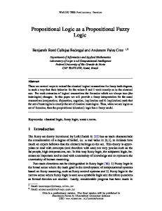
3D. Metatheorems and rules of deduction. The Deduction Theorem is an example of a metatheorem for PL, a theorem about formal proofs which can be used to show that formal proofs exist without actually constructing them. Diagram 1 on the next page lists several useful metatheorems of this

Math. 114L, Spring 2016, Y. N. Moschovakis Propositional Calculus March 6, 2016, 20:03, 11

12

THE PROPOSITIONAL CALCULUS PL

type, including the following three—whose proofs, incidentally, illustrate the usefulness of the Deduction Theorem: 3D.1. Lemma (simp1 ). If T, ¬φ ` φ, then T ` φ. Proof. The hypothesis and the Deduction Theorem give us a proof from T of ¬φ → φ, and we start with this and continue as follows: from T : . . . , ¬φ → φ, (¬φ → φ) → [(¬φ → ¬φ) → ¬¬φ] (Axiom 3), (¬φ → ¬φ) → ¬¬φ (Modus Ponens), . . . , ¬φ → ¬φ (inserting the proof from Lemma 3B.1), ¬¬φ (Modus Ponens), ¬¬φ → φ (Axiom 4), φ (Modus Ponens).

a

3D.2. Lemma (¬-introduction). If T, φ ` ¬÷, then T, ÷ ` ¬φ. Proof. We assume given a proof of ¬÷ from T, φ, and then the Deduction Theorem 3C gives us a proof of φ → ¬÷ from T , which is also a proof from T, ÷. We start with this proof and continue as follows: from T, ÷ : . . . , φ → ¬÷, ÷ → (φ → ÷) (Axiom 1), ÷ (Hyp), φ → ÷ (Modus Ponens), (φ → ÷) → [(φ → ¬÷) → ¬φ] (Axiom 3), (φ → ¬÷) → ¬φ (Modus Ponens), ¬φ (Modus Ponens). a 3D.3. Lemma (¬ elimination). If T ` φ, then for every ÷, T, ¬φ ` ÷. Proof. The hypothesis gives us a proof of φ from T which is also a proof of φ from T, ¬φ; we start with this and continue with applications of axioms and Modus Ponens as follows: from T, ¬φ : . . . , φ, φ → (¬÷ → φ), ¬÷ → φ ¬φ, ¬φ → (¬÷ → ¬φ), ¬÷ → ¬φ (¬÷ → φ) → [(¬÷ → ¬φ) → ¬¬÷] (Modus Ponens twice)¬¬÷, ¬¬÷ → ÷, ÷.

a

We understand the sequents T ` φ in this system of rules Gs as claims that there is a proof of φ from T . Thus the basic hypothesis sequent ÷ ` ÷ simply says that (hypothesis)

there is a deduction of ÷ from ÷,

which is trivial; the thinning rule says that (thinning) if there is a deduction of ÷ from T , then there is a deduction of ÷ from T, φ,

Math. 114L, Spring 2016, Y. N. Moschovakis Propositional Calculus March 6, 2016, 20:03, 12

13

THE PROPOSITIONAL CALCULUS PL

÷ ` ÷ (hypothesis) T `÷ T, φ ` ÷

T, φ ` ¬÷ T, ÷ ` ¬φ T `φ

T `φ∧ø

T, ÷ ` φ T `÷→φ

T `φ

T `φ∨ø

T ` ¬φ T `φ T, ¬φ ` ÷

T, φ ` ÷ T, φ ∧ ø ` ÷

(∧-intro)

T `ø

T, φ ` ¬φ

(simp1 )

(¬-intro)

T `ø

T `φ T `φ∨ø

T, ¬φ ` φ

(thinning)

(∨-intro)

T, φ ` ÷

T `φ

T, φ ∧ ø ` ÷ T, ø ` ÷

T `ø

(∧-elim)

(∨-elim)

T, ø ` ÷

T, φ → ø ` ÷ T, φ ` ø

(¬-elim)

T, ø ` ÷

T, φ ∨ ø ` ÷ T `φ

(→-intro)

(simp2 )

(→-elim)

(Cut)

Diagram 1. The system Gs which is also trivial and the (simp1 ), (¬-intro) and (¬-elim) rules are exactly Lemmas 3D.1 – 3D.3. The three structural rules in the second level of the system express very simple properties of the provability relation ` and the cut which comprises the third group is essentially equivalent to Modus Ponens. Notice the symmetry in the middle group of logical rules: for each connective • there is an introduction rule which helps to prove formulas in which • is the main connective, and an elimination rule which suggests how we can use a hypothesis in which • is the main connective. The Deduction Theorem is tagged →-introduction. 3D.4. Theorem (Soundness of Gs ). All the rules in the list Gs are valid. We will skip the complete proof which involves constructing several arguments like those in the proofs of Lemmas 3D.1 – 3D.3; this is tedious but very useful, because the use of these rules often make it very easy to prove that formal proofs exist. In fact much more (and interesting) is true of Gs , but we do not need it here and we will leave (some of) it for the last Section 4.

Math. 114L, Spring 2016, Y. N. Moschovakis Propositional Calculus March 6, 2016, 20:03, 13

14

THE PROPOSITIONAL CALCULUS PL

We now turn to the proof of the Completeness Theorem, for which we need one (important) definition and two lemmas. 3D.5. Definition (Consistency and strong completeness). A set of formulas T is consistent if there is no formulas ÷ such that T ` ÷ and T ` ¬÷; is is strongly complete if for every formula ÷, either ÷ ∈ T or ¬÷ ∈ T . 3D.6. Lemma. A set of formulas S is consistent and strongly complete if and only if there is an assignment v to the propositional variables such that for every formula φ, (3-2)

v |= φ ⇐⇒ φ ∈ S.

Proof. If (3-2) holds for S and some v, then S is obviously strongly complete since for every φ, either v |= φ or v |= ¬φ. To see that it is also consistent, notice that by the Soundness Theorem 3B, S ` φ =⇒ S |= φ =⇒ v |= φ, which with (3-2) eliminates the possibility that for some φ, S ` φ and also S ` ¬φ. For the converse, we assume that S is consistent and strongly complete. Notice first that that S is closed under deduction, i.e., (3-3)

S ` φ =⇒ φ ∈ S;

because if S ` φ but φ ∈ / S, then ¬φ ∈ S by the strong completeness, and so S ` ¬φ which makes it inconsistent. With this in mind, set v(p) = 1 ⇐⇒ p ∈ S and prove (3-2) by induction on φ. It is true at the basis (when φ is a propositional variable) by the definition of v, and to consider just two of the cases at the induction step: v |= ¬φ ⇐⇒ v 6|= φ ⇐⇒ φ ∈ / S (ind. hyp) ⇐⇒ ¬φ ∈ S (strong completeness), v |= φ ∧ ø ⇐⇒ v |= φ and v |= ø ⇐⇒ φ ∈ S and ø ∈ S ⇐⇒ φ ∧ ø ∈ S the last step by (3-3), since φ, ø ` φ ∧ ø and φ ∧ ø ` φ, φ ∧ ø ` ø.

a

3D.7. Lemma. Every consistent set T of formulas can be extended to a consistent, strongly complete T ∗ ⊇ T .

Math. 114L, Spring 2016, Y. N. Moschovakis Propositional Calculus March 6, 2016, 20:03, 14

15

THE PROPOSITIONAL CALCULUS PL

Proof. The key observation is that for every consistent set S and any formula ÷, one of the two sets S ∪ {÷},

S ∪ {¬÷}

is consistent, cf. Problem x1.22. The idea is to extend T by adding to it successively each formula or its negation until we get in the end the required strongly complete, extension T ∗ . In detail, let Fn be the set of formulas of length ≤ n + 1 in which only the variables A0 , . . . , An may occur, e.g., F0 = {A0 }. This set is finite, for every n, so we can fix an enumeration Fn = {÷0n , . . . , ÷knn } of it. Lining up these enumerations in sequence, one after another, we obtain an enumeration (with many irrelevant repetitions) ÷0 , ÷ 1 , . . . of all PL-formulas, which we fix. We now define a sequence of sets T0 ⊆ T1 ⊆ T2 · · · by setting recursively T0 = T,

(

Tn+1 =

Tn ∪ {÷n } if Tn ∪ {÷n } is consistent, Tn ∪ {¬÷n } otherwise, S

so that (inductively) each Tn is consistent and so T ∗ = n Tn ⊇ T is consistent by Problem x1.23, and it is obviously strongly complete. a 3E. The Completeness Theorem for PL. (1) Every consistent set of formulas is satisfiable. (2) For every set of formulas T and every ÷, if T |= ÷, then T ` ÷. Proof. (1) follows immediately by the two Lemmas: extend T to a consistent, strongly complete T ∗ ⊇ T by Lemma 3D.7 and then apply Lemma 3D.6. (2) Assume, towards a contradiction that T |= ÷ but T 6` ÷. It follows that the set T ∪ {¬÷} is consistent, since if T, ¬÷ ` φ and T, ¬÷ ` ¬φ, then T ` ¬¬÷ by Problem x1.17 and hence T ` ÷, which contradicts the hypothesis. So there is an assignment v which satisfies every formula in T ∪ {¬÷} by (1), contradicting the assumption T |= ÷. a It is Part (2) which is properly called the Completeness Theorem, but Part (1) is more useful for many applications.

Math. 114L, Spring 2016, Y. N. Moschovakis Propositional Calculus March 6, 2016, 20:03, 15

16

THE PROPOSITIONAL CALCULUS PL

§4. Some results about Gs . We can think of the system Gs as a formal system which proves sequents T ` φ—exactly those sequents which are true of the Hilbert system by the next theorem. It is a simplified version of a classical deduction system created by Gerhard Gentzen in the 1930s which is the basic tool of Proof Theory, the part of logic which studies the structure of proofs. 4.1. Theorem (Proof theoretic completeness of Gs ). If T ` ÷, then there is a proof of this using the Gs -rules. Proof. Without giving a precise definition of a formal Gs -proof, we give such proofs of some of the Hilbert axioms as examples of how such proofs can be constructed. First for axioms (4), (1) and (5): ¬÷ ` ¬÷ ¬¬÷, ¬÷ ` ÷ ¬¬÷ ` ÷

(thinning) (simp1 )

` (¬¬÷) → ÷ φ`φ φ, ø ` φ

(→-intro)

(thinning)

φ`φ φ, ø ` φ

(thinning)

φ`ø→φ

(→-intro)

` φ → (ø → φ) ø`ø φ, ø ` ø

φ, ø ` φ ∧ ø φ ` ø → (φ ∧ ø)

(→-intro)

(thinning) (∧-intro)

(→-intro)

` φ → (ø → (φ ∧ ø))

(→-intro)

This last Gs -proof for Axiom (5) is in tree form, because of the application of the two-premise (∧-intro) rule. This is most often the case. In the next (and more complex) Gs -proof of Axiom (2), we skip the labelling with the rules, but we box the active formulas which determine which rule is applied in each case. We also allow different sets of side formulas in the premises of rules, which is justified as long as we include all of them in the conclusion. For example, we can justify this stronger version of ∧-introduction T2 , ` ø T1 ` φ T1 ` φ T2 , ` ø as an abbreviation of T1 , T2 ` φ T1 , T2 ` ø T1 , T 2 ` φ ∧ ø T1 , T2 ` φ ∧ ø which has some additional thinnings. This is done once in this Gs -proof of Axiom (2):

Math. 114L, Spring 2016, Y. N. Moschovakis Propositional Calculus March 6, 2016, 20:03, 16

THE PROPOSITIONAL CALCULUS PL

ø` ø φ` φ φ` φ

17

÷ `÷

ø, ø → ÷ ` ÷

φ, ø , φ → (ø → ÷) ` ÷

φ , φ → ø, φ → (ø → ÷) ` ÷ φ → ø, φ → (ø → ÷) ` φ → ÷ φ → ø ` φ → (ø → ÷) → (φ → ÷) ` (φ → ø) → ((φ → (ø → ÷)) → (φ → ÷)) As a last example we give a Gs -proof of Axiom (3): ¬ø ` ¬ø φ`φ ø ` ¬¬ø φ, φ → ø ` ¬¬ø φ`φ φ, ¬ø ` ¬(φ → ø) φ → ¬ø, φ ` ¬(φ → ø) φ → ø, φ → ¬ø ` ¬φ φ → ø ` (φ → ¬ø) → ¬φ ` (φ → ø) → [(φ → ¬ø) → ¬φ] Notice that these Gs -proofs of the Hilbert axioms do not use the Cut Rule. This is needed to verify the Modus Ponens rule, that [T ` φ and T ` φ → ø] =⇒ T ` ø, whose verification is as follows: ø`ø T `φ T `φ→ø

T, ø ` ø

T, φ → ø ` ø T `ø

(thinnings) (→-elim)

(Cut)

a

The system Gs is a simplified version of a classical deduction system created by Gerhard Gentzen in the 1930s which is the basic tool of Proof Theory, the part of logic which studies the structure of proofs. Gentzen-style systems have many “nice” properties, including the fundamental (and surprizing) fact that the cut rule is not needed—every sequent T ` φ which is provable using the rules of Gs can be proved without using cuts. This is not easy to prove, but just knowing it helps to discover Gs proofs of given sequents. §5. Problems. x1.1. Prove that the set of propositional formulas defined in 1A.1 is the smallest set of strings which is propositionally closed; i.e., it is propositionally closed and it is a subset of every propositionally closed set of strings.

Math. 114L, Spring 2016, Y. N. Moschovakis Propositional Calculus March 6, 2016, 20:03, 17

18

THE PROPOSITIONAL CALCULUS PL

x1.2. A sequence α0 , . . . , αk of strings is a propositional formula construction if for each n ≤ k, either αn is a propositional variable, or αn ≡ (¬αi ) for some i < n, or αn ≡ (αi • αj ) for some binary connective • and some i, j < n. Prove that a string of symbols φ is a propositional formula if and only if it occurs in some propositional formula construction. x1.3. Prove (2) of Lemma 1A.2, that for every non-empty, proper, initial part α of a formula φ, the number of left parentheses “(” in α is greater than the number of right parentheses “)” in α. x1.4∗ (Parsing Lemma for PL). Prove Theorem 1A.3. Hint: For the most interesting part (3) of the uniqueness claim, suppose (ø1 •1 ÷1 ) ≡ (ø2 •2 ÷2 ) with ø1 shorter than ø2 and derive a contradiction using Lemma 1A.2. x1.5. For each of the following equations between strings, determine whether there are formulas φ, ø, ÷, φ 0 , ø 0 , ÷ 0 which make them true: (a) ((φ ∧ ø) ∨ ÷) ≡ (φ 0 ∨ (ø 0 ∧ ÷ 0 )). (b) ((φ ∧ ø) ∨ ÷) ≡ (φ 0 ∧ (ø 0 ∨ ÷ 0 )). You must prove your answers. x1.6. Let ↓ be the Sheffer stroke, the binary connective defined by the truth table p q p↓q 0 0 1 0 1 0 1 0 0 1 1 0 We read (φ ↓ ø) as “neither φ nor ø”. Define the ↓-formulas using only this connective (rather than ¬, ∧, ∨, →, ↔), and prove that every n-ary bit function can be defined by a ↓-formula with n propositional variables. x1.7. Prove Lemma 2A.1. x1.8. Prove the Tarski conditions, Theorem 2C.1. x1.9. Prove equation (2-3) in the proof of the Replacement Theorem 2D.1, i.e., the following: for every formula φ whose variables are in the list p1 , . . . , pk , if q~ ≡ q1 , . . . , ql is a sequence of distinct variables which include all the variables in ø1 , . . . , øk , y ~ ≡ y1 , . . . , yl and ÷ ≡ φ{p1 :≡ ø1 , . . . , pk :≡ øk }, then (∗)

F÷,~q (~ y ) = Fφ,~p (Fø1 ,~q (~ y ), . . . , Føk ,~q (~ y )).

Math. 114L, Spring 2016, Y. N. Moschovakis Propositional Calculus March 6, 2016, 20:03, 18

19

THE PROPOSITIONAL CALCULUS PL

x1.10. Prove that the formula (2) in Theorem 2D.2 is a tautology. x1.11. Prove that the formula (8) in Theorem 2D.2 is a tautology. x1.12. Prove Lemma 2D.3, the Modus Ponens Rule. x1.13. Prove that if T, φ |= ø, then T |= φ → ø. 5.2. Definition. For any finite sequence of formulas ÷0 , ÷1 , . . . , ÷n , set W W

i≤n ÷i

so that, for example W W

i≤0 ÷i

≡ ÷0 ,

W W

i≤1 ÷i

:≡ ÷0 ∨ ÷1 ∨ · · · ∨ ÷n ≡ ÷0 ∨ ÷1 ,

W W

i≤2 ÷i

≡ ÷0 ∨ ÷1 ∨ ÷2 .

Similarly for abbreviation of finite conjunctions: V V

i≤n ÷i

:≡ ÷0 ∧ ÷1 ∧ · · · ∧ ÷n

x1.14∗ . Suppose R(i, j) is a relation defined for i, j ≤ n, choose a doubly indexed sequence of distinct propositional variables {pij }i,j≤n , and consider the assignment (

v(pij ) =

1, if R(i, j), 0, otherwise.

The variables {pij } can be used to express various properties about the relation R. Recall for example that R is symmetric ⇐⇒ (for all i, j ≤ n)[R(i, j) ⇐⇒ R(j, i)]; now easily, R is symmetric ⇐⇒ v |=

V V

V V i≤n

j≤n [pij

↔ pji ].

Find similar formulas which express the following properties of R: (a) R is the graph of a function, i.e., (R(i, j) & R(i, k)) =⇒ j = k. (b) R is the graph of a one-to-one function. (c) R is the graph of a surjection—a function from {0, . . . , n} onto {0, . . . , n}. x1.15. Prove Lemma 3A.1, that for every T and every φ, T ` φ ⇐⇒ φ ∈ S for every deductively closed S ⊇ T x1.16. Prove that the “repetition” clause (D2) in the definition of deduction is not needed: i.e., if T ` ÷, then there is a deduction of ÷ from T without repetitions. (The clause was included in the definition so that we can most combine deductions without restriction.) x1.17 (Proof by contradiction). Prove that if T, ÷ ` φ and T, ÷ ` ¬φ, then T ` ¬÷.

Math. 114L, Spring 2016, Y. N. Moschovakis Propositional Calculus March 6, 2016, 20:03, 19

20

THE PROPOSITIONAL CALCULUS PL

x1.18. Construct a Gs proof of the propositional axiom scheme (8), i.e., the formula (φ → ÷) → ((ø → ÷) → ((φ ∨ ø) → ÷)) x1.19. Prove that if T is not consistent, then T ` ÷ for every ÷. x1.20. Prove in Gs the following classical rule of ¬-elimination: T, ¬φ ` ÷ (¬-elimC) T, ¬÷ ` φ x1.21∗ (The law of excluded middle). Prove that for every formula ÷, ` ÷ ∨ ¬÷. Hint: Using the classical rule of ¬-elimination in Problem x1.20, give a Gs -proof of ¬(÷ ∨ ¬÷) ` (÷ ∨ ¬÷) and then apply simp1 . x1.22. Prove that if T is a consistent set of formulas, then for every ÷, one of the two sets T ∪ {÷},

T ∪ {¬÷}

is consistent. x1.23. Prove that a set of formulas T is consistent if and only if every finite subset of T is consistent. x1.24∗ . Construct a Gs proof of Peirce’s Law, the formula (((p → q) → p) → p) Hint: Show p ` (((p → q) → p) → p) and ¬p ` (((p → q) → p) → p), and then use ∨-elimination and the Law of Excluded Middle Problem x1.21∗ . (And there are many other ways to do this—none of them quite trivial.) x1.25. Two formulas φ and ø are (logically) equivalent if φ |= ø and ø |= φ. Prove that for each sequence p1 , . . . , pn of distinct propositional variables, there is a sequence n

÷1 , . . . , ÷N with N = 22

of inequivalent formulas in the variables p1 , . . . , pn , such that every formula in which only these variables occur is equivalent to some ÷i . (For example, when n = 1, the required sequence is p, ¬p, p ∧ p, p ∨ ¬p.) Hint: Count truth tables. x1.26 (The Compactness Theorem for PL). Suppose T is an infinite set of formulas. Prove that if every finite subset T0 ⊂ T of T is satisfiable, then T is satisfiable.

Math. 114L, Spring 2016, Y. N. Moschovakis Propositional Calculus March 6, 2016, 20:03, 20