3
households’ choices chapter 7
utility and demand What shapes an individual’s demand? Why is demand elastic for some goods and inelastic for others?
chapter 8
possibilities, pre f e rences, and choices How can we predict the effects of changes in prices and incomes on what people buy, how much they work, and how much they borrow and lend?
3
3
uti lity an d demand
3
OBJECTIVES After studying this chapter, you will be able to:
t m Explain the relationship between individual demand and market demand
t m Describe the budget constraint and identify its impact on household choices
t m
Understand how the concepts of total and marginal utility are used to define preferences, another determinant of household choices
t m
Explain how consumers make choices by maximizing their utility (called the marginal utility theory)
t m Use the marginal utility theory to predict the effects of changing prices and income
t m
Appreciate the criticisms of marginal utility theory
t m Understand how to calculate consumer surplus, and how to explain the paradox of value
KEY TERMS Consumer equilibrium, 151 Diminishing marginal utility, 149 Marginal utility, 149
Marginal utility per dollar spent, 151 Utility, 148 Value, 158
K E Y F I G U R E S A N D TA B L E S
m n Figure 7.1 n m Figure 7.2 n m Figure 7.3 n m Figure 7.4 n m Figure 7.5 n m Figure 7.6 m n Figure 7.7 n m Table 7.3
Individual and Market Demand Curves, 147
n m
Marginal Utility Theory, 157
Table 7.7
Consumption Possibilities, 148 Total Utility and Marginal Utility, 150 Equalizing the Marginal Utility per Dollar Spent, 153 A Fall in the Price of Movies, 154 A Rise in the Price of Soft Drink, 155 Consumer Surplus, 159 Maximizing Utility by Equalizing Marginal Utilities per Dollar Spent, 152
PA RT 3 H O U S E H O L D S ’ C H O I C E S
We need water to live. We don’t need diamonds for much besides decoration. If the benefits of water far outweigh the benefits of diamonds, why, then, does water cost practically nothing while diamonds are terribly expensive? When OPEC restricted its sale of oil in 1973, it created a dramatic rise in price, but people continued to use almost as much oil as they had before. Our demand for oil was inelastic. But why? In 1985, soon after CD players first became available, the price tag was $650 — more than $1,000 in today’s money — and consumers were reluctant to buy them. Since then, the price has decreased dramatically, and people are buying them in enormous quantities. Our demand for CD players is elastic. What makes the demand for some things elastic while the demand for others is inelastic? Over the past decade, after removing the effects of inflation, incomes have increased by 35 per cent. Over that same period, expenditure on food has increased by 26 per cent, while expenditure on health has increased by 55 per cent. The proportion of income spent on health has increased and the proportion spent on food has decreased. Why, as incomes rise, does the proportion of income spent on some goods rise and on others fall? In the last three chapters, we’ve seen that demand has an important role in the determination of prices. But we have not analysed what exactly shapes a person’s demand. This chapter does that. In doing so, it also explains why demand is elastic for some goods and inelastic for others, and why the prices of some things, such as diamonds and water, are so out of proportion to their benefits.
I N D I V I D UAL DE MAND A ND MA RKE T DEM AND The total quantity demanded of a good at a particular price in a market will be made up of the quantities demanded by all the individuals who are buying at that price. This means that the market demand curve is related to individual demand curves. This connection is important to understand because market demand curves matter for price determination but their features depend on those of the individual demand curves. Later in this chapter we’ll spend more time on the determinants of an individual’s demand curve. The table in Fig. 7.1 illustrates the relationship between individual demand and market demand. In this example, Lisa and Alex are the only people in the market. The market demand is therefore the total demand of Lisa and Alex. At $3 a movie, Lisa demands 5 movies and Alex 2, so that the total quantity demanded by the market is 7 movies. Similarly, at a higher price, say $4, Lisa demands 4 movies and Alex 1, so total demand is 5 movies. The market demand is formed by adding together the individual demands. 146
Figure 7.1 illustrates the relationship between individual and market demand curves. Part (c) plots the market demand at each price. It is the sum of the demand curves of Lisa and Alex. Lisa’s demand curve for movies in part (a) and Alex’s in part (b) sum horizontally to the market demand curve in part (c). W H AT IS THE RELAT IONS HIP BET WEEN I N D I V I D UA L AN D M AR KET D EM AND ?
n Market demand is the relationship between the total quantity of a good demanded and its price. n Individual demand is the relationship between the quantity of a good demanded by a single individual and its price. n The market demand curve is the horizontal sum of the individual demand curves formed by adding the quantities demanded by each individual at each price. HOUSEH OLD CONSUM PTION CHOICES The next step is to investigate an individual demand curve. We do this by studying how a single household makes its consumption choices.
CHAPTER 7 UT ILITY AND DEMAN D
FI GUR E 7.1 Ind ivid ual an d M ar ket Dem and Cur ve s
Price of a movie (dollars)
Lisa
7 6 5 4 3 2
1 2 3 4 5 6
Quantity of movies demanded Alex Market 0 0 0 1 2 3
1 2 3 5 7 9
A household’s consumption choices are determined by many factors, but we can summarize all of these factors under two concepts: n Budget constraint n Preferences BUDGET CONSTRAINT A household’s consumption choices are constrained by its income and by the prices of the goods and services it buys. Households have a given amount of income to spend and cannot influence the prices of the goods and services they buy. Households take prices as given. The limits to a household’s consumption choices are described by its budget line. To make the concept of the household’s budget line as clear as possible, we’ll consider the example of Lisa, who has an income of $30 a month to spend. She buys two goods — movies and soft drink. Movies cost $6 each; soft drink costs $3 a litre. If Lisa spends all of her income, she will reach the limits to her consumption of movies and soft drink.
The table and diagram illustrate how the quantity of movies demanded varies as the price of a movie varies. In the table, the market demand is the sum of the individual demands. For example, at a price of $3, Lisa demands 5 movies and Alex demands 2 movies, so the total quantity demanded in the market is 7 movies. In the diagram, the market demand curve is the horizontal sum of the individual demand curves. Thus when the price is $3, the market demand curve shows that the quantity demanded is 7 movies, the sum of the quantities demanded by Lisa and Alex.
In Fig. 7.2, each row of the table shows an affordable way for Lisa to consume movies and soft drink. Row a indicates that she can buy 10 litres of soft drink and see no movies. You can see that this combination of movies and soft drink exhausts her monthly income of $30. Row f says that Lisa can watch 5 movies and have no soft drink — another combination that exhausts the $30 available. Each of the other rows in the table also exhausts Lisa’s income. (Check that each of the other rows costs exactly $30.) The numbers in the table define Lisa’s consumption possibilities. We can graph Lisa’s consumption possibilities as points a to f in Fig. 7.2. Lisa’s budget line is a constraint on her choices. It marks the boundary between what is affordable and what is unaffordable. She can afford all the points on the line and inside it. She cannot afford points outside the line. The constraint on her consumption depends on prices and on her income, and the constraint changes when prices and her income change. 147
PA RT 3 H O U S E H O L D S ’ C H O I C E S
UTILITY AN D PRE FERE NCE S
F IGU RE 7. 2 Co nsu mpti on Po s s i b i l i t i e s
Movies Expenditure Quantity (dollars) a b c d e f
0 1 2 3 4 5
0 6 12 18 24 30
The other determinant of household choices is preferences. Preferences are used to answer questions such as: ‘How does Lisa divide her $30 between these two goods?’ The answer depends on her likes and dislikes — on her preferences. The benefit or satisfaction that a person gets from the consumption of a good or service is called utility. But what exactly is utility and in what units can we measure it? This question is the topic of this section, and in the next we’ll see how the concept of utility can be used to explain how consumers make choices.
Soft drink Expenditure Total Litres (dollars) expenditure 10 8 6 4 2 0
30 24 18 12 6 0
30 30 30 30 30 30
Six possible ways of allocating $30 to movies and soft drink are shown as the rows a to f in the table. For example, Lisa can buy 2 movies and 6 litres (row c). Each row shows the combinations of movies and soft drink that cost $30. These possibilities are points a to f in the figure. The line through those points is a boundary between what Lisa can afford and cannot afford. Her choices must lie inside the orange area or along the line af.
H OW DO ES THE BUD G ET CONS TRAI NT AFFE CT H OUS EHOL D CH OICES ?
n A household’s consumption choices are constrained by its income and by the prices of the goods and services it buys. n This constraint is described by its budget line. n The budget line marks the boundary between what is affordable and what is unaffordable.
148
T E M P E R ATURE — AN ANALOGY Utility is an abstract concept and its units are arbitrary. Temperature is an abstract concept and the units of temperature are arbitrary. You know when you feel hot and you know when you feel cold. But you can’t observe temperature. You can observe water turning to steam if it’s hot enough or turning to ice if it’s cold enough. You can construct an instrument, called a thermometer, that will tell you how hot or cold it is. The scale on the thermometer is what we call temperature. But the units in which we measure temperature are arbitrary. For example, we can accurately predict that when a Celsius thermometer shows a temperature of 0°, water will turn to ice. But the units of measurement do not matter because this same event also occurs when a Fahrenheit thermometer shows a temperature of 32°. The concept of utility helps us make predictions about consumption choices in much the same way that the concept of temperature helps us make predictions about physical phenomena. It has to be admitted, though, that the theory which does this is not as precise as the theory that enables us to predict when water will turn to ice or steam. TOTAL UTILITY Total utility is the total benefit or satisfaction that a person gets from the consumption of goods and services. Total utility depends on the person’s level of consumption — more consumption gives more total utility. Table 7.1 shows Lisa’s total utility from consuming different quantities of movies and soft drink. If she sees no movies, she gets no utility from movies. If she sees 1 movie in a month, she gets 50 units of utility. As the number of movies
C HA PTER 7 UTIL ITY AND DEMAND
TA B L E 7 . 1 L i s a ’s Total Uti lity from Mov ie s an d So ft D ri nk
Movies Quantity per month
Total utility
0 1 2 3 4 5 6 7 8 9 10
0 50 88 121 150 175 196 214 229 241 250
Soft drink Litres per month Total utility 0 1 2 3 4 5 6 7 8 9 10
0 75 117 153 181 206 225 243 260 276 291
she sees in a month increases, her total utility increases so that if she sees 10 movies a month, she gets 250 units of total utility. The other part of the table shows Lisa’s total utility from soft drink. If she drinks no soft drink, she gets no utility. As the amount of soft drink she consumes rises, her total utility increases. MARGINAL UTILITY Marginal utility is the change in total utility resulting from a one-unit increase in the quantity of a good consumed. The table in Fig. 7.3 shows the calculation of Lisa’s marginal utility of movies. When her consumption of movies increases from 4 to 5 movies a month, her total utility from movies increases from 150 units to 175 units. Thus for Lisa, the marginal utility of seeing a fifth movie each month is 25 units. Notice that marginal utility appears midway between the quantities of consumption. It does so because it is the change in consumption from 4 to 5 movies that produces the marginal utility of 25 units. The table displays calculations of marginal utility for each level of movie consumption. Figure 7.3(a) illustrates the total utility that Lisa gets from movies. As you can see, the more movies Lisa sees in a month, the more total utility she gets. Part (b) illustrates her marginal utility. This graph tells us that as Lisa sees more movies, the marginal utility that she gets from watching movies decreases. For example, her marginal utility from the first movie is 50 units, from the second, 38
units, and from the third, 33 units. We call this decrease in marginal utility as the consumption of a good increases the principle of diminishing marginal utility. Figure 7.3 illustrates an important relationship between total and marginal utility. Marginal utility is equal to the slope of the total utility curve. As the total utility curve becomes flatter at the top in part (a), and its slope declines, the marginal utility also falls. At low levels of consumption, when the total utility curve is steeper, the marginal utility is higher. This relationship between marginal and total values is not unique to utility. We will discover it again in other settings — for example, in determinants of costs of production in Chapter 10. Marginal utility is positive but generally diminishes as the consumption of a good increases. Why does marginal utility have these two features? In Lisa’s case, she likes movies, and the more she sees the better. That’s why marginal utility is positive. The benefit that Lisa gets from the last movie seen is its marginal utility. To see why marginal utility diminishes, think about how you’d feel in the following two situations. In one, you’ve just been studying for 29 evenings in a row. An opportunity arises to see a movie. The utility you get from that movie is the marginal utility from seeing one movie in a month. In the second situation, you’ve been on a movie binge. For the past 29 nights, you have not even seen an assignment or a test. You are up to your eyeballs in movies. You are happy enough to go to a movie on yet one more night. But the thrill that you get out of that 30th movie in 30 days is not very large. It is the marginal utility of the 30th movie in a month and is less than the marginal utility of your 29th trip to the movies. H OW C A N PREF ER E NCES BE DE SCRI BE D BY U TILI T Y?
n Consumers’ preferences are described by using the concept of utility — the total benefit or satisfaction that a consumer gets from a good or service. n The greater the quantity of a good consumed, the higher is the total utility from consuming that good. n As the quantity of a good consumed increases, the marginal utility from consuming that good decreases — the principle of diminishing marginal utility. n Utility is an abstract concept and its units of measurement are arbitrar y. 149
PA RT 3 H O U S E H O L D S ’ C H O I C E S
FI GURE 7.3 To tal Util ity and Mar ginal Ut ili ty
The table shows that as Lisa’s consumption of movies increases, so does the utility she derives from movies. The table also shows her marginal utility — the change in utility resulting from the last movie seen. Marginal utility declines as consumption increases. Lisa’s utility and marginal utility from
MAXIM IZIN G UTILITY Now that we’ve defined utility and examined its measurement, we can apply the concept to the question of how households make choices. Households consume the quantities of goods and services that maximize total utility. A household’s income and the prices it faces limit the utility that it can obtain. In making choices, households have to take into consideration the income available for spending and the prices faced. Lisa allocates her spending between movies and soft drink to maximize her total utility. To see how she does that, we’ll continue to assume that movies 150
Quantity
Total utility
Marginal utility
1 2 3 4 5
50 88 121 150 175
50 38 33 29 25
movies are graphed in the figure. Part (a) shows total utility. It also shows the extra utility gained from each additional movie — marginal utility — as a bar. Part (b) shows the diminishing marginal utility from movies by placing the bars shown in part (a) side by side in declining steps.
cost $6 each, soft drink costs $3 a litre, and Lisa has $30 a month to spend. THE UTILITY-MAXIMIZING CHOICE To calculate how Lisa spends her money if she maximizes her total utility, make a table like the one shown in Table 7.2. The table shows all Lisa’s affordable combinations of movies and soft drink, together with the total utility she gets from each combination. The table shows the same affordable combinations of movies and soft drink found on Lisa’s budget line in Fig. 7.2. It records, first, the number of movies consumed and the total
CHAPTE R 7 U TILITY AND DEMA ND
utility derived from them (the left side of the table); second, the number of litres of soft drink consumed and the total utility derived from them (the right side); and third, the total utility derived from both movies and soft drink (the middle column). In the first row of Table 7.2, Lisa watches no movies and buys 10 litres of soft drink. In this case, she gets no utility from movies and 291 units of total utility from soft drink. Her total utility from movies and soft drink (the centre column) is 291 units. The rest of the table is constructed in the same way. The consumption of movies and soft drink that maximizes Lisa’s total utility is highlighted in the table. When Lisa consumes 2 movies and 6 litres of soft drink, she gets 313 units of total utility. This is the best Lisa can do given that she has only $30 to spend and given the prices of movies and litres. If she buys 8 litres of soft drink, she can see only 1 movie and gets 310 units of total utility, 3 less than the maximum attainable. If she sees 3 movies and drinks only 4 litres, she gets 302 units of total utility, 11 less than the maximum attainable. What we’ve just described is a consumer equilibrium. A consumer equilibrium is a situation in which a consumer has allocated his or her income in the way that maximizes total utility. In finding Lisa’s consumer equilibrium, we measured her total utility from the consumption of movies and soft drink. There is a better way of determining a consumer equilibrium, which does not involve measuring total utility at all. Let’s look at this alternative, which is called the marginal utility theory of consumer choice. E Q UALIZING MARGINAL UTILITY PER DOLLAR SPENT Lisa has money to spend on movies and soft drink. Movies cost $6 each. Soft drink costs $3. Is it worth giving up a movie in order to buy two soft drinks? Lisa will do that if the utility gained from the extra soft drink exceeds that lost on the movies. Lisa is asking the question — can I reallocate my budget to raise more utility? The answer depends on the utility yielded from Lisa’s budget dollars in their different uses. The yield of utility from a dollar of Lisa’s budget depends on two things: the marginal utility of the good bought, and the number of units of a good which can be bought. The second of these, the number of units which can be bought, depends on the price of the good.
TA B L E 7 . 2 L i s a ’s Affo rd a ble C omb inat i ons o f M ovi es and So ft Dr ink
Movies Quantity Total utility 0 1 2 3 4 5
Total utility from movies and soft drink
0 50 88 121 150 175
291 310 313 302 267 175
Soft drink Total utility Litres 291 260 225 181 117 0
10 8 6 4 2 0
Important variables in this approach to determining a consumer equilibrium are therefore marginal utility and price. They are combined in the following general rule. The allocation that maximizes a consumer’s total utility is the one that makes the marginal utility per dollar spent on each good equal for all goods. The marginal utility per dollar spent is the marginal utility obtained from the last unit of a good consumed divided by the price of the good. For example, Lisa’s marginal utility from consuming the first movie is 50 units of utility. The price of a movie is $6, which means that the marginal utility per dollar spent on movies is 50 units divided by $6, or 8.33 units of utility per dollar. Total utility is maximized when all the consumer’s income is spent and when the marginal utility per dollar spent is equal for all goods. Lisa maximizes total utility when she spends all her income and consumes movies and soft drink such that Marginal utility 0from movies0 Price of movies
5
Marginal utility 0from soft drink0 Price of soft drink
Call the marginal utility from movies MUm, the marginal utility from soft drink MUs, the price of movies Pm, and the price of soft drink Ps. Then Lisa’s utility is maximized when she spends all her income and when MUm MUs }} 5 }} Pm Ps Let’s use this formula to find Lisa’s utilitymaximizing allocation of her income. Table 7.3 sets out Lisa’s total and marginal utilities per dollar spent for both movies and soft 151
PA RT 3 H O U S E H O L D S ’ C H O I C E S
drink. For example, in row b Lisa’s marginal utility from the first movie is 50 units and, since movies cost $6 each, her marginal utility per dollar spent on movies is 8.33 units per dollar (50 units divided by $6). When Lisa is consuming 8 litres of soft drink, her marginal utility is 17 units. This is the extra utility gained from increasing soft drink consumption from 7 to 8 units — that is, the difference between 260 and 243 units of utility. (These numbers are found from Table 7.1 and are shown in brackets in the marginal utility column for movies in Table 7.3.) The marginal utility per dollar spent on soft drink is then 5.67 (17 units divided by $3). Each row in Table 7.3 contains an allocation of Lisa’s income that uses up her $30. You can see that Lisa’s marginal utility per dollar spent on each good, like marginal utility itself, decreases as consumption of the good increases. Total utility is maximized when the marginal utility per dollar spent on movies is equal to the marginal utility per dollar spent on soft drink — possibility c, where Lisa consumes 2 movies and 6 litres — the same allocation as we calculated in Table 7.2. Figure 7.4 shows why the rule ‘equalize marginal utility per dollar spent on all goods’ works. Suppose that instead of consuming 2 movies and 6 litres (possibility c), Lisa consumes 1 movie and 8 litres (possibility b). She then gets 8.33 units of utility from the last dollar spent on
movies and 5.67 units from the last dollar spent on soft drink. In this situation it pays Lisa to spend less on soft drink and more on movies. If she spends a dollar less on soft drink and a dollar more on movies, her total utility from soft drink decreases by 5.67 units and her total utility from movies increases by 8.33 units. Lisa’s total utility increases if she spends less on soft drink and more on movies. Or, suppose that Lisa consumes 3 movies and 4 litres of soft drink (possibility d). In this situation, her marginal utility per dollar spent on movies is less than her marginal utility per dollar spent on soft drink. Lisa can now get more total utility by cutting her spending on movies and increasing her spending on soft drink. UNITS OF UTILITY The calculations of the utility-maximizing allocation of income in Table 7.3 and Fig. 7.4 have been performed using marginal utility and price. By making the marginal utility per dollar spent equal for both goods, we know that Lisa has maximized her total utility. This way of viewing maximum utility is important; it means that the units in which utility is measured do not matter. We could double or halve all the numbers measuring utility, or multiply them by any other positive number, or square them, or take their square roots. None of these transformations of the units used to measure utility
TABLE 7.3 M axim izing Utili ty by Eq ual izi ng Ma rg in al Utili tie s pe r Do lla r S pe nt
Movies ($6 each) Quantity a
0
Total utility 0
Marginal utility
Soft drink ($3 per litre) Marginal utility per dollar spent
0
Litres
Total utility
10
291
Marginal utility 15
Marginal utility per dollar spent 5.00
(= 291–276)
b
1
50
50
8.33
8
260
17
5.67
(= 260–243)
c
2
88
38
6.33
6
225
19
6.33
(= 225–206)
d
3
121
33
5.50
4
181
28
9.33
(= 181–153)
e
4
150
29
4.83
2
117
42
14.00
(= 117–75)
f 152
5
175
25
4.16
0
0
CHAPTE R 7 U TILITY AND DEMA ND
F IGURE 7. 4 E qua liz ing t he M arg in al Util ity pe r Do lla r Spent
n When marginal utilities per dollar spent are equal for all goods, a consumer cannot reallocate spending to get more total utility. n This is called the marginal utility theory of consumer choice. PREDICTIONS OF MARGINAL UTILI TY THEORY We’ll now use marginal utility theory to make some predictions. What happens to Lisa’s consumption of movies and soft drink when their prices change and when her income changes?
If Lisa consumes 1 movie and 8 litres of soft drink (possibility b), she gets 8.33 units of utility from the last dollar spent on movies and 5.67 units of utility from the last dollar spent on soft drink. She can get more total utility by buying one more movie. If she consumes 4 litres and 3 movies (possibility d), she gets 5.50 units of utility from the last dollar spent on movies and 9.33 units of utility from the last dollar spent on soft drink. She can get more total utility by buying one fewer movie. When Lisa’s marginal utility per dollar spent on both goods is equal, her total utility is maximized.
make any difference to the outcome. It is in this respect that utility is analogous to temperature. Our prediction about the freezing of water does not depend on the temperature scale; our prediction about maximizing utility does not depend on the units of utility. H OW DO C ONSUM ER S MAKE C HOICES BY M AXI MI ZI NG UT ILI TY?
n Consumers maximize total utility. n They do so by spending all the available income and by making the marginal utility per dollar spent on each good equal.
A FALL IN THE PRICE OF MOV I E S To determine the effect of a change in price on consumption requires three steps: n First, determine the combinations of movies and soft drink that can be bought at the new prices. n Second, calculate the new marginal utilities per dollar spent. n Third, determine the consumption of each good that makes the marginal utility per dollar spent on each good equal and that just exhausts the money available for spending. Table 7.4 shows the combinations of movies and soft drink that exactly exhaust Lisa’s $30 of income when movies cost $3 each and soft drink costs $3 a litre. Lisa’s preferences do not change when prices change, so her marginal utility schedules remain the same. But now we divide her marginal utility from movies by $3, the new price of a movie, to get the marginal utility per dollar spent on movies. What is the effect of the fall in the price of a movie on Lisa’s consumption? You can find the answer by comparing her new utility-maximizing allocation (Table 7.4) with her original allocation (Table 7.3). Lisa responds to a fall in the price of a movie by watching more movies (up from 2 to 5 a month) and drinking less soft drink (down from 6 to 5 litres a month). That is, Lisa substitutes movies for soft drink when the price of a movie falls. Figure 7.5 illustrates these effects. In part (a) a fall in the price of movies produces a movement along Lisa’s demand curve for movies, and in part (b) it shifts her demand curve for soft drink. A RISE IN THE PRICE OF SOFT DRINK Table 7.5 shows the combinations of movies and soft drink that exactly exhaust her $30 of income
153
PA RT 3 H O U S E H O L D S ’ C H O I C E S
TABLE 7.4 H ow a Ch ange in the P rice of Movi es A ffe cts Li sa ’s Ch o ic es
Movies ($3 each)
Soft drink ($3 per litre)
Quantity
Marginal utility
Marginal utility per dollar spent
Litres
0 1 2 3 4 5 6 7 8 9 10
50 38 33 29 25 21 17 15 12 9
16.67 12.67 11.00 9.67 8.33 7.00 6.00 5.00 4.00 3.00
10 9 8 7 6 5 4 3 2 1 0
Marginal utility 15 16 17 18 19 25 28 36 42 75
Marginal utility per dollar spent 5.00 5.33 5.67 6.00 6.33 8.33 9.33 12.00 14.00 25.00
FI GURE 7.5 A Fa ll i n th e Price of M ov i e s
When the price of movies falls and the price of soft drink remains constant, the quantity of movies demanded by Lisa increases; in part (a), Lisa moves along her demand curve for
movies. Also, Lisa’s demand for soft drink decreases; in part (b), her demand curve for soft drink shifts to the left.
when movies cost $3 each and soft drink costs $6 a litre. Now we divide her marginal utility from soft drink by $6, the new price of a litre, to get the marginal utility per dollar spent on soft drink. The effect of the rise in the price of soft drink on Lisa’s consumption is seen by comparing her
new utility-maximizing allocation (Table 7.5) with her previous allocation (Table 7.4). Lisa responds to a rise in the price of soft drink by drinking less soft drink (down from 5 to 2 litres a month) and watching more movies (up from 5 to 6 a month). That is, Lisa substitutes movies for soft drink when
154
C HAPTER 7 UTIL ITY AND DEMAND
TA B L E 7 . 5 H ow a Chan ge in the Pri ce of Sof t Dr in k Af fec ts Lis a’s Choi ces
Movies ($3 each) Quantity 0 2 4 6 8 10
Soft drink ($6 per litre)
Marginal utility
Marginal utility per dollar spent
Litres
38 29 21 15 9
12.67 9.67 7.00 5.00 3.00
5 4 3 2 1 0
the price of soft drink rises. Figure 7.6 illustrates these effects. In part (a) a rise in the price of soft drink produces a movement along Lisa’s demand curve for soft drink, and in part (b) it shifts her demand curve for movies. Marginal utility theory predicts these two results: when the price of a good rises, the quantity demanded of that good decreases; if the price of one good rises, the demand for another good that can serve as a substitute increases. Does this sound familiar? It should. These predictions of marginal
Marginal utility
Marginal utility per dollar spent
25 28 36 42 75
4.17 4.67 6.00 7.00 12.50
utility theory correspond to the assumptions that we made about consumer demand in Chapter 4. There we assumed that the demand curve for a good sloped downward, and we assumed that a rise in the price of a substitute increased demand. Marginal utility theory predicts these responses to price changes. In doing so it makes three assumptions. First, that consumers maximize total utility. Second, that they get more utility as they consume more of a good. Third, that as consumption increases, marginal utility declines.
F IGURE 7. 6 A R ise in the Pric e o f Sof t Drin k
When the price of soft drink rises and the price of movies remains constant, the quantity of soft drink demanded by Lisa decreases; in part (a), Lisa moves along her demand curve for
soft drink. Also, Lisa’s demand for movies increases; in part (b), her demand curve for movies shifts to the right.
155
PA RT 3 H O U S E H O L D S ’ C H O I C E S
A RISE IN INCOME Suppose that Lisa’s income increases to $42 a month and that movies cost $3 each and a litre of soft drink costs $3 (as in Table 7.4). We saw, in Table 7.4, that with these prices and with an income of $30 a month, Lisa consumes 5 movies and 5 litres of soft drink a month. We want to compare this consumption of movies and soft drink with Lisa’s consumption at an income of $42. The calculations for the comparison are shown in Table 7.6. With $42, Lisa can buy 14 movies a month and no soft drink, or 14 litres of soft drink a month and no movies, or any combination of the two goods as shown in the table. We calculate the marginal utility per dollar spent in exactly the same way as we did before and find the quantities at which the marginal utilities per dollar spent on movies and on soft drink are equal. With an income of $42, the marginal utility per dollar spent on each good is equal when Lisa watches 7 movies and drinks 7 litres of soft drink a month. By comparing this situation with that in Table 7.4, we see that with an additional $12 a month, Lisa consumes 2 more litres and 2 more movies. This response arises from Lisa’s preferences, as described by her marginal utilities. Different
preferences produce different quantitative responses. But for normal goods, a higher income always brings a larger consumption of all goods. For Lisa, soft drink and movies are normal goods. When her income increases, Lisa buys more of both goods. MARGINAL UTILITY AND CONSUMER CHOICES The marginal utility theory is summarized in Table 7.7. This theory can be used to answer a wide range of questions about the real world, some of which were posed at the beginning of this chapter. Why is the demand for CD players elastic and the demand for oil inelastic; and why, as income increases, does the proportion of income spent on electricity increase while the proportion spent on transportation decreases? These patterns in our spending result from the rate at which our marginal utility for each good diminishes as its consumption is increased. Goods whose marginal utilities diminish rapidly have inelastic demands (e.g. oil). For example, when the price of a good falls, the consumer will increase their purchases. When marginal utility falls rapidly, just a small increase in consumption will equalize the marginal utilities per dollar spent. In
TAB LE 7 .6 L i s a ’s C hoic es wi th an Inc o me o f $ 42 a Mon th
Movies ($3 each) Quantity 0 1 2 3 4 5 6 7 8 9 10 11 12 13 14 156
Soft drink ($3 per litre)
Marginal utility
Marginal utility per dollar spent
50 38 33 29 25 21 17 15 12 9
16.67 12.67 11.00 9.67 8.33 7.00 6.00 5.00 4.00 3.00
Litres 14 13 12 11 10 9 8 7 6 5 4 3 2 1 0
Marginal utility
15 16 17 18 19 25 28 36 42 75
Marginal utility per dollar spent
5.00 5.33 5.67 6.00 6.33 8.33 9.33 12.00 14.00 25.00
CHAPTER 7 UTILITY AND DEMAND
that case, the percentage change in quantity demanded will be less and so the demand curve will be less elastic. A good whose marginal utility falls rapidly will also show a small income effect (e.g. transportation). A rise in income will lead to an increase in quantity demanded, but quantity demanded increases by a smaller amount when marginal utility declines rapidly. Goods whose marginal utility diminish only slowly, on the other hand, have elastic demands (e.g. oil) and large income effects (e.g. electricity). W H AT DOE S THE M ARGINA L U TILI TY T H E O RY P RED IC T WI LL BE THE E FFECTS OF CH ANGE S I N PRI CES AND INC OMES?
n When the price of a good falls and the prices of other goods remain constant, consumers increase their consumption of the good whose price has fallen and decrease their demand for other goods. n Other things being equal, a price change results in a movement along the demand curve for a good whose price has changed and in a shift in the demand cur ves for other goods whose prices have remained constant. n When a consumer’s income increases, the consumer can afford to buy more of all goods and the quantity bought increases for all normal goods. n Goods whose marginal utility diminishes rapidly
have inelastic demands and small income effects; goods whose marginal utility diminishes slowly have elastic demands and large income effects. CRITIC ISM S OF MARG IN AL UTILITY T H E O RY Marginal utility theory helps us to understand the choices people make, but there are some criticisms of this theory. ‘UTILITY CAN’T BE OBSERVED OR MEASURED’ Agreed — we can’t observe utility. But we don’t need to observe it to use it. We can and do observe the quantities of goods and services that people consume, the prices of those goods and services, and people’s incomes. Our goal is to understand the consumption choices that people make and to predict the effects of changes in prices and incomes on these choices. To make such predictions, we assume that people derive utility from their consumption, that more consumption yields more utility, and that marginal utility diminishes. From these assumptions, we make predictions about the directions of change in consumption when prices and incomes change. We are building a model and using that model to predict behaviour. In order to make progress in that exercise, we use the concept of utility.
TABLE 7. 7 M argi nal Util ity Theo ry
Assumptions (a) A consumer derives utility from the goods consumed. (b) Each additional unit of consumption yields additional utility; marginal utility is positive. (c) As the quantity of a good consumed increases, marginal utility decreases. Implication Utility is maximized when all the available income is spent and when the marginal utility per dollar spent is equal for all goods. Predictions (a) Other things being equal, the higher the price of a good, the lower is the quantity bought (the law of demand). (b) The higher the price of a good, the higher is the consumption of substitutes for that good. (c) The higher the consumer’s income, the greater is the quantity demanded of normal goods. 157
PA RT 3 H O U S E H O L D S ’ C H O I C E S
Furthermore, as we’ve already seen, the actual numbers that might be used to express utility do not matter. Consumers maximize utility in this model by making the marginal utility per dollar spent on each good equal. As long as the same scale is used to express utility for all goods, the model gives the same answer regardless of the units on the scale. In this regard, utility is similar to temperature — water freezes when it’s cold enough, and that occurs independently of the temperature scale used. We don’t have to use a particular scale in order to get the model to work for us. ‘PEOPLE AREN’T THAT CLEVER’ Some critics maintain that marginal utility theory assumes that people are supercomputers. It requires people to look at the marginal utility of every good at every different quantity they might consume, divide those numbers by the prices of the goods, and then calculate the quantities so as to equalize the marginal utility of each good divided by its price. Such criticism of marginal utility theory once again confuses the actions of people in the real world with those of people in a model economy. A model economy is no more an actual economy than a model railway is an actual railway. The people in the model economy perform the calculations that we have just described. People in the real world just consume. We observe their consumption choices, not their mental gymnastics. The marginal utility theory proposes that the consumption patterns we observe in the real world are similar to those implied by the model economy in which people do compute the quantities of goods that maximize utility. We test how closely the marginal utility model resembles reality by checking the predictions of the model against observed consumption choices. W H AT ARE THE CR ITIC ISM S O F TH E M ARG INAL U TIL IT Y T HE ORY ?
n One criticism is that utility can’t be measured: that is true, but as long as we use the same scale to express utility for all goods, we’ll get the same predictions from the theory regardless of the units on our scale. n ‘People aren’t that clever’ says another criticism: maybe so, but we can test how closely the marginal utility model resembles reality by checking the predictions of the model against observed consumption choices. 158
I M P L I C ATIONS OF MARGINAL UT IL IT Y TH EORY We all love bargains — paying less for something than its usual price. One implication of the marginal utility theory is that we almost always get a bargain when we buy something. That is, we place a higher total value on the things we buy than the amount it costs us. CONSUMER SURPLUS AND THE GAINS F ROM TRADE People can gain by specializing in the production of the things at which they have a comparative advantage and then trading with each other. Marginal utility theory gives us a way of measuring the gains from trade. When Lisa buys movies and soft drink, she exchanges her income for them. Does Lisa profit from this exchange? Are the dollars she has to give up worth more or less than the movies and soft drink are worth to her? The principle of diminishing marginal utility guarantees that Lisa, and everyone else, gets more value from the things they buy than the amount of money they give up in exchange. C A L C U L ATING CONSUMER SURPLUS The value a consumer places on a good is the maximum amount that person would be willing to pay for it. The amount actually paid for a good is its price. Consumer surplus is the difference between the value of a good and its price. The definition of consumer surplus was discussed in Chapter 6 (p. 131). Diminishing marginal utility guarantees that a consumer always makes some consumer surplus. To understand why, let’s look again at Lisa’s consumption choices. As before, assume that Lisa has $30 a month to spend, that movies cost $3 each, and that she watches 5 movies each month. Now look at Lisa’s demand curve for movies, shown in Fig. 7.7(a). We can see from Lisa’s demand curve that if she were able to watch only 1 movie a month, she would be willing to pay $7 to see it. She would be willing to pay $6 to see a second movie, $5 to see a third, and so on. These decreases in her willingness to pay reflect the declining marginal utilities from the consumption of extra movies. Luckily for Lisa, she has to pay only $3 for each movie she sees — the market price of a movie. Although she values the first movie she sees in a
CHAPTE R 7 U TILITY AND DEMA ND
F IGURE 7. 7 Con su mer Sur pl us
In part (a), Lisa is willing to pay $7 for the first movie, $6 for the second, $5 for the third, $4 for the fourth, and $3 for the third. She pays $3 for each movie and has a consumer surplus on the first four movies equal to $10 ($4 + $3 + $2 + $1). In part (b), the entire market has a consumer surplus of $12.5 million, as shown by the area of the green triangle.
month at $7, she pays only $3, which is $4 less than she would be willing to pay. The second movie she sees in a month is worth $6 to her. The difference between the value she places on the movie and what she has to pay is $3. The third movie she sees in a month is worth $5 to her,
which is $2 more than she has to pay for it, and the fourth movie is worth $4, which is $1 more than she has to pay for it. You can see this progression in Fig. 7.7(a), which highlights the difference between the price she pays ($3) and the higher value she places on the first, second, third, and fourth movies. These differences are a gain to Lisa. The next step is to calculate her total gain. The total amount that Lisa is willing to pay to see the 5 movies is $25 (the sum of $7, $6, $5, $4, and $3). She actually pays $15 (5 movies multiplied by $3). The extra value she receives from the movies is therefore $10. This amount is the value of Lisa’s consumer surplus. From watching 5 movies a month, she gets $10 worth of value in excess of what she has to spend to see them. Suppose there are a million consumers similar to, but not quite identical to, Lisa. Some are willing to pay $8 for the first movie. At $7.99, yet more movies are demanded. And as the price falls a cent at a time, the quantity of movies demanded increases. For the market as a whole, the consumer surplus is the entire area under the demand curve and above the market price line, as shown in Fig. 7.7(b). Extracting from consumers a greater part of their consumer surplus is a challenge for many entrepreneurs. We look at the example of ‘the scalper’ in Reading Between the Lines on pp. 162–3, who thrives on the mistakes apparently made by others! THE PA R A D OX OF VA L U E More than 200 years ago, Adam Smith posed the paradox that we raised at the start of this chapter. Water, which is essential to life itself, costs little; but diamonds, which are useless compared to water, are expensive. Why? Adam Smith could not solve the paradox. Not until the theory of marginal utility had been developed could anyone give a satisfactory answer. You can solve Adam Smith’s puzzle by distinguishing between total utility and marginal utility. The total utility that we get from water is enormous. But remember, the more we consume of something, the smaller is its marginal utility. We use so much water that the marginal utility — the benefit we get from one more glass of water — diminishes to a tiny value; diamonds, on the other hand, have a small total utility relative to water, but because we buy few diamonds, they have a high marginal utility. 159
PA RT 3 H O U S E H O L D S ’ C H O I C E S
Marginal utility theory predicts that consumers spend their income in a way that makes the marginal utility from each good divided by its price equal for all goods. This also holds true for their spending on diamonds and water: diamonds have a high marginal utility divided by a high price, while water has a low marginal utility divided by a low price. In each case, the marginal utility per dollar spent is the same. W H AT ARE SOME I MP L ICATI ONS O F TH E MAR GINAL UTI LITY T HEORY ?
n Willingness to pay declines with the quantity purchased because of diminishing marginal utility. n Diminishing marginal utility guarantees that a consumer always makes some consumer surplus. n The paradox of value can be explained by the difference between total and marginal utility. n Something essential to life (like water) has a high total utility but low marginal utility and may have a low value because consumers are willing to pay little for it. LOOKING AHEAD We’ve now completed our study of the marginal utility theory of consumption. We’ve used that theory to examine how Lisa allocates her income between the two goods that she consumes — movies and soft drink. We’ve also seen how the theory can be used to resolve the paradox of value. Furthermore, we’ve seen how the theory can be used to explain our consumption choices. In the next chapter we’ll study an alternative theory of household behaviour. To help you see the connection between the marginal utility theory of this chapter and the more modern theory of consumer behaviour of the next chapter, we’ll continue with the same example and discover another way of understanding how Lisa gets the most out of her $30 a month.
I N D I V I D UAL DEMAND AND M AR KET DEMAND
Individual demand is the relationship between the price of a good and the quantity demanded by a single individual. Market demand is the sum of all individual demands, and the market demand curve is found by summing horizontally all the individual demand curves. (p. 146) HOUS EHO LD CONS UMPTI ON CH OICE S AND TH E BU DGET C O NSTR A IN T
An individual demand curve is derived from a household’s consumption choices. These choices are constrained by its income and by the prices of the goods and services it buys. This constraint is described by its budget line. It marks the boundary between what is affordable and what is unaffordable. (pp. 146–8) UTILI TY AND HOU SEHO LD PREFERENCES
Consumers’ preferences are described by using the concept of utility. The consumer derives utility from the goods consumed, and the consumer’s total utility increases as consumption of the good increases. The change in total utility resulting from a one-unit increase in the consumption of a good is called marginal utility. Marginal utility declines as consumption increases. (pp. 148–50) M AXIM IZING UTI LITY
The consumer’s goal is to maximize total utility, given the income available to be spent and given the prices of the goods and services bought. Utility is maximized when all the available income is spent and when the marginal utility per dollar spent on each good is equal. This way of determining a consumer equilibrium is called the marginal utility theory of consumer choice. (pp. 150–3) 160
C HAPTER 7 UTIL ITY AND DEMAND
PRE DICTION S OF MARGI NA L U TILI TY T H E O RY
Marginal utility theory predicts how prices and income affect the amounts of each good consumed. First, it predicts the law of demand. That is, other things being equal, the higher the price of a good, the lower is the quantity demanded of that good. Second, it predicts that, other things being equal, the higher the consumer’s income, the greater is the consumption of all normal goods. (pp. 153–7) C RITI CI SM S OF MAR GINA L UTI LITY T H E O RY
Some people criticize marginal utility theory because utility cannot be observed or measured. However, the size of the units of measurement of utility does not matter. All that matters is that the ratio of the marginal utility from each good to its price is equal for all goods. Any units of measurement consistently applied will do. The concept of utility is analogous to the concept of temperature — it cannot be directly observed, but it can be used to make predictions about events that are observable. Another criticism of marginal utility theory is that consumers can’t be as clever as the theory implies. In fact, the theory makes no predictions about the thought processes of consumers. It only makes predictions about their actions and assumes that people spend their income in what seems to them to be the best possible way. (pp. 157–8) I M P L I C ATIONS OF MAR GINAL UTI LIT Y T H E O RY
Marginal utility theory implies that every time we buy goods and services we get more value for our expenditure than the money we spend. We benefit from consumer surplus, which is equal to the difference between the maximum amount that we are willing to pay for a good and the price that we actually pay. Marginal utility theory resolves the paradox of value: water is extremely valuable to life but cheap, while diamonds are less valuable to life though expensive. When we talk loosely about value, we are thinking of total utility. The total utility of water is higher than the total utility of diamonds. The marginal utility of water, though, is lower than the marginal utility of diamonds. People choose the amount of water and diamonds to consume so as to maximize
total utility. In maximizing total utility, they make the marginal utility per dollar spent the same for water as for diamonds. (pp. 158–60) RE VIEW QUESTI ONS 1 What is the relationship between individual demand and market demand? 2 How do we construct a market demand curve from individual demand curves? 3 What do we mean by utility? 4 Distinguish between total utility and marginal utility. 5 How does marginal utility change as the level of consumption of a good changes? 6 Susan is a consumer. When is Susan’s utility maximized? a) When she has spent all her income b) When she has spent all her income and marginal utility is equal for all goods c) When she has spent all her income and the marginal utility per dollar spent is equal for all goods Explain your answer. 7 What does the marginal utility theory predict about the effect of a change in price on the quantity of a good consumed? 8 What does the marginal utility theory predict about the effect of a change in the price of one good on the consumption of another good? 9 What does the marginal utility theory predict about the effect of a change in income on consumption of a good? 10 How would you answer someone who says that the marginal utility theory is useless because utility cannot be observed? 11 How would you respond to someone who tells you that the marginal utility theory is useless because people are not clever enough to compute a consumer equilibrium in which the marginal utility per dollar spent is equal for all goods? 12 What is consumer surplus? How is consumer surplus calculated? 13 What is the paradox of value? How does the marginal utility theory resolve it?
161
Consumer surplus at work
Angry fans in jam after ‘scalping’ By ADAM HARVEY
F
ans have claimed that scalpers have robbed them of the chance to buy cheap tickets for Pearl Jam, one of the rock industry’s most popular acts, which will tour Australia next month. While most rock bands say they owe it all to their fans, it seemed that for once, a major act was prepared to forgo huge profit for the benefit of concertgoers. Pearl Jam tickets were $36.80, including a booking fee — below the usual price for a top act. But fans claim scalpers bought most of the tickets minutes after they went on sale. Pearl Jam’s Sydney Entertainment Centre concert sold out within five minutes, and all 30,000 tickets for the band’s Eastern Creek concert went in three hours. All but two Pearl Jam concerts sold out within three hours. Melanie Lyn, 17, of Carlingford, a regular concertgoer, was fourth in line at a Hornsby ticket agent — but when she got to the
162
counter, Pearl Jam’s Entertainment Centre concert was sold out. She bought tickets for Eastern Creek, but by then, even that concert was half-sold. ‘We had people in front of us buying 500 tickets — which meant that only three people got tickets at Hornsby . . . We go to every concert that comes out because we love music, but you always get scalpers at these things,’ she said. ‘Every single concert we’ve gone to, we’ve been sold bad seats, because scalpers buy up the tickets almost as soon as they go on sale.’ In an industry where decent seats often sell for up to $150, Pearl Jam has a reputation for being fanfriendly. It has taken the US ticketing agent Ticketmaster to court for alleged anti-competitive behaviour, and insists on low prices. Melanie says Pearl Jam’s Australian promoters, Frontier Touring, should have imposed a limit of four tickets per person. She
is organising a protest against its policy, outside the Entertainment Centre concert on March 10. Frontier claims that scalping is not a problem, and that limits on tickets are unnecessary. Tickets were sold through 54 box offices and 110 phone lines, so, of course, they sold exceptionally quickly, a Frontier spokesperson said. But Triple J has received almost 200 calls from people claiming they saw scalpers buying Pearl Jam tickets. One scalper called to say he had bought 75 tickets. Scalping is not illegal. But under the Prices Regulation Act, anyone who sells tickets for more than 5 per cent above their retail price can be prosecuted. The NSW Department of Consumer Affairs used to prosecute scalpers before 1989, but says it is no longer worth it. Sydney Morning Herald 18 February 1995
ESSE NCE OF THE S TO RY
n
n Pearl Jam concert tickets were priced at just under $40. n All but two concerts in Sydney sold out in less than three hours. n Fans claimed that scalpers were buying large blocks of tickets for resale and wanted limits put on the number of tickets which each person could buy. n The expected price for good seats when the tickets were resold by the scalpers was $150.
n
A N A LYS I S
n
n Seats at Pearl Jam concerts are scarce. As shown in the figure, the market clearing price ($150) is high. People are willing to pay high prices because the utility of hearing Pearl Jam play live is high. n Concert promoters often decide to keep seat prices low, and lower than the market clearing price, for example at $40. There are about 40,000 tickets for sale for the Sydney concerts. At that price there is excess demand for seats. n The market works by using other devices to ration the tickets available. n One of these is queuing. People queue up — they sleep overnight outside the booking office before it opens — to be sure to get a ticket. n There are costs of queuing which have to be added to the ticket price to estimate the full cost of a seat at the concert. Those who obtain seats are likely to be people with a relatively low cost of queuing. n There is scope for trade between the people who obtain the tickets by queuing and those who are willing to pay higher money
n n
n
n
prices but who do not have tickets. This possibility leads to the second method of allocation, which is scalping. Some people buy tickets at low prices (and incur costs of queuing in the process) and resell at the market clearing price. Scalping is more likely to lead to an allocation of the available seats to people whose willingness to pay lies to the left of point f. Scalping provides the means by which seats are reallocated to those who are willing to pay more for them. Why are the ticket prices so low? Why does the promoter not try to capture more of the surplus available by offering seats at a higher price? One explanation is that the promoter does not want to take the risk of not filling the concert. A half-empty hall or stadium could send the wrong signal about the popularity of the band. People’s willingness to listen to bands may depend on their perception of the band’s popularity with others. The promoter wants to fill the hall, so prices are set low to make that outcome more likely. That creates the opportunity for scalpers, who take the risk that they cannot sell all the tickets they have bought. They therefore bear some of the risk that the promoter has decided to avoid. A second explanation is that the concert is not the only product which the promoters and the band are selling. They also sell complementary products such as CDs and clothing. The sales of these items will be increased, it is argued, as a result of greater numbers at the concert. It may also be thought that the people
n n
n
n
who queue for tickets have a greater propensity to buy this sort of material than those who would be willing to pay a high price. A third explanation is that there is a conflict of interest between the band and the promoter. The band may want to retain the loyalty of fans, especially those with a high propensity to buy recorded music. Those fans are then more likely to buy other products released some time later, like the next CD. High concert prices, and a perception that the band is not ‘fan-friendly’, may diminish the band’s popularity and reduce future sales of CDs. Low sales reduce the income of the band. It also reduces the extent to which their music is available now and the extent to which it ‘survives’ the band. Apart from income, longevity may be an objective of the musicians! Compared to the band, the concert will put a higher weight on current revenue than on revenue from future concerts, the likelihood of which is difficult to estimate. This difference may be a source of disagreement between the promoter and the band.
163
PA RT 3 H O U S E H O L D S ’ C H O I C E S
P RO B L E M S 1
Shirley’s demand for yoghurt is given by the following: Price (dollars per carton)
Quantity (cartons per week)
1 2 3 4 5
12 9 6 3 1
1 2 3 4 5
6 5 4 3 2
b) Draw a graph of Dan’s demand curve. c) If Shirley and Dan are the only two individuals, construct the market demand schedule for yoghurt. d) Draw a graph of the market demand for yoghurt. e) Draw a graph to show that the market demand cur ve is the horizontal sum of Shirley’s demand curve and Dan’s demand curve. 2
3
164
Calculate Lisa’s marginal utility from soft drink from the numbers given in Table 7.1. Draw two graphs, one of her total utility and the other of her marginal utility from soft drink. Make your graphs look similar to those in Fig. 7.3. Alex enjoys windsurfing and snorkelling. He obtains the following utility from each of these sports:
Utility from snorkelling
1 2 3 4 5 6 7 8 9
60 110 150 180 200 206 211 215 218
20 38 53 64 70 75 79 82 84
b) Compare the two utility graphs. Can you say anything about Alex’s preferences?
Dan also likes yoghurt. His demand for yoghurt is given by the following: Quantity (cartons per week)
Utility from windsurfing
a) Draw graphs showing Alex’s utility from windsurfing and from snorkelling.
a) Draw a graph of Shirley’s demand for yoghurt.
Price (dollars per carton)
Half-hours per month
c) Draw graphs showing Alex’s marginal utility from windsurfing and from snorkelling. d) Compare the two marginal utility graphs. Can you say anything about Alex’s preferences? 4
Alex has $35 to spend. Equipment for windsurfing rents for $10 a half-hour, while snorkelling equipment rents for $5 a half-hour. Use this information, together with that given in problem 3, to answer the following questions: a) What is the marginal utility per dollar spent on snorkelling if Alex snorkels for: (i) Half an hour? (ii) One and a half hours? b) What is the marginal utility per dollar spent on windsurfing if Alex windsurfs for: (i) Half an hour? (ii) One hour? c) How long can Alex afford to snorkel if he windsurfs for: (i) Half an hour? (ii) One hour? (iii) One and a half hours? d) Will Alex choose to snorkel for one hour and windsurf for one and a half hours? e) How long will Alex choose to windsurf and to snorkel?
C HAPTER 7 UTIL ITY AND DEMAND
5
Alex’s sister gives him $20 to spend on his leisure pursuits, so he now has $55 to spend. a) How long will Alex now windsurf and snorkel? b) If Alex has only $55 to spend and the rent on windsurfing equipment halves to $5 a halfhour, how will Alex now spend his time windsurfing and snorkelling? c) Does Alex’s demand cur ve for windsurfing slope downward or upward? d) Alex takes a holiday in the Whitsundays, the cost of which includes unlimited sports activities — including windsurfing, snorkelling, and tennis. There is no extra charge for any equipment. Alex decides to spend three hours each day on both windsurfing and snorkelling.
How long does he windsurf? How long does he snorkel? 6
Sara’s demand for windsurfing is given by: Price (dollars per half-hour)
Time windsurfing (half-hours per month)
12.50 15.00 17.50 20.00
8 6 4 2
a) If windsurfing costs $17.50 a half-hour, what is Sara’s consumer surplus? b) If windsurfing costs $12.50 a half-hour, what is Sara’s consumer surplus?
165