Essays on the Political Economy of Finance Thomas Lambert

To cite this version: Thomas Lambert. Essays on the Political Economy of Finance. Economies and finances. Universit´e du Droit et de la Sant´e - Lille II, 2015. English. .

HAL Id: tel-01192769 https://tel.archives-ouvertes.fr/tel-01192769 Submitted on 3 Sep 2015

HAL is a multi-disciplinary open access archive for the deposit and dissemination of scientific research documents, whether they are published or not. The documents may come from teaching and research institutions in France or abroad, or from public or private research centers.

L’archive ouverte pluridisciplinaire HAL, est destin´ee au d´epˆot et `a la diffusion de documents scientifiques de niveau recherche, publi´es ou non, ´emanant des ´etablissements d’enseignement et de recherche fran¸cais ou ´etrangers, des laboratoires publics ou priv´es.

Essays on the Political Economy of Finance

Thomas LAMBERT Doctoral Thesis 01 | 2015

Université catholique de Louvain

Université Lille 2

LO U V A I N S C H O O L O F M A NA G E M E NT R E S E A R C H I NS T I T U T E

DR OI T E T S A NT É

´ catholique de Louvain Universite ´ Lille 2 Universite

Doctoral Thesis

Essays on the Political Economy of Finance

Thomas Lambert

A thesis submitted in fulfilment of the requirements for the degree of Doctor of Philosophy in Economics and Management

Jury Members:

Advisors: Prof. Paul Belleflamme Prof. Armin Schwienbacher

Prof. Marco Becht Prof. Enrico Perotti Prof. Paolo Volpin

Chairman: Prof. Per Agrell

XX

February 11, 2015

UNIVERSITE CATHOLIQUE DE LOUVAIN UNIVERSITE LILLE 2

Abstract Essays on the Political Economy of Finance by Thomas Lambert

What are the consequences of countries’ political system on their financial markets and intermediaries? This dissertation proceeds in answering this question along three essays. The first essay focuses on the way suffrage institutions, a key measure of the distribution of political power, shape countries’ reliance on both stock market and bank finance. It provides evidence from the last two centuries that suffrage expansions adversely affect stock market development, consistent with the insight that small elites pursue economic opportunities by promoting capital raised on stock markets. In contrast, it shows a positive effect of suffrage on banking development, consistent with the idea that an empowered middle class favors banks as they share its aversion for risk. The second essay examines the political outcomes driving the pace and extent of financial reforms occurring in the last three decades around the world. It stresses the role of government cohesiveness in explaining patterns of financial liberalizations, finding that fragmented governments do breed stalemate. The third essay explores the incidence and drivers of lobbying efforts made by the U.S. banking industry. It shows that banks engage in lobbying to gain preferential treatment, and take in turn additional risks. Thomas Lambert (Namur, 1984) holds a Master degree in economics from the Universit´e catholique de Louvain. Thomas is a teaching assistant at the Louvain School of Management and a PhD candidate in finance jointly at the Universit´e catholique de Louvain and Universit´e Lille 2. In 2013, he was a visiting scholar at the London Business School. His research interests mainly lie between political economics and corporate finance, but Thomas has also side interests in entrepreneurial finance. His work has been presented in leading academic conferences such as the American Economic Association, the European Finance Association, and the American Law and Economics Association along with various other places, including Bocconi, Cambridge, CES Munich, HEC Paris, LBS, PSE, Queen’s Belfast, and Tilburg. Prior to pursuing a PhD, Thomas worked as a consultant at Ernst & Young, Brussels.

Acknowledgements In writing this thesis, I am very fortunate to have enjoyed insights, guidance and support from a large number of people. Highlighting individuals runs the great risk of erroneously omitting others equally deserving my gratitude. However, my education in finance has taught me that risks should sometimes be taken. First of all, I would like to thank my supervisors, Paul Belleflamme and Armin Schwienbacher. Paul kindly agreed to supervise me when Armin left the Universit´e catholique de Louvain. Asking to a theoretical IO Professor to supervise a thesis in finance might seem surprising, but Paul was a natural choice to me. When we worked together on “Crowdfunding: Tapping the Right Crowd”, a paper developed in parallel of this thesis, I have learned an incredible amount about how to conduct meaningful research and, more specifically, about the IO approach to the theoretical definition of economic problems. Paul was also always available whenever I was in need of guidance and reading drafts of my papers. Paul contributed, probably more than he would think, to my current way of viewing the economics (and finance) discipline. As for Armin, I literally would not be here without him. He gave me the opportunity to join the Louvain School of Management (LSM) and, later, the European Centre for Corporate Control Studies (ECCCS) in Lille. He initiated me to the realm of corporate finance, and then provoked (by any chance?) my curiosity and admiration towards the institutional and political economics approach to finance. Armin’s expertise and guidance proved to be very fruitful in developing my own research ideas which he supported and helped me expand during our many enjoyable discussions, mostly in his car to commute to Lille. His trust in my capacities and potential have been empowering and motivating. Without any doubts, this dissertation would not be what it is without his support, patience and effort, which deserve all my gratitude. Together with my supervisors, I am also grateful to the jury members for their invaluable contribution to the scientific development of this dissertation. In fact, I had the privilege of being assigned a jury in which every member played a crucial role in shaping my research. Marco Becht came on board during an intermediate stage of my PhD, namely the ´epreuve de confirmation. This first meeting turned out to be extremely useful for the research agenda developed in this dissertation. I had the pleasure of having him constructively criticizing my research papers, their relevance and methods. As for Paolo Volpin, he had a significant impact on my work, either through his own research or various informal interactions. I had the pleasure to meet him at the London Business School (LBS), where he kindly acted as my local supervisor for an eight-months research visit. I am grateful for his valuable comments on my research and for his time taken to discuss and challenge my ideas. As for Enrico Perotti, I had fewer occasions to meet iii

iv him in person than the other members of the jury, but his pioneering research on the political economy of finance has been a source of constant inspiration from the earliest stages of my PhD. I take advantage of this occasion to deeply thank Enrico for his encouragements and support. A sincere thank to Per Agrell for being the president of my jury. Other professors also had a significant impact on my education attainment, even though they were not in my jury. Of course, Hans Degryse deserves very special thanks. Besides co-authoring “The Political Economy of Financial Systems: Evidence from Suffrage Reforms in the Last Two Centuries”, he read my Job Market Paper in huge detail, and without fail would provide a stream of insightful comments. I particularly valued Hans’s openness in giving (quickly) critical feedback which increased the precision and accuracy of my work. In addition, Hans provided a substantial amount of broader advice on the academic profession, which will guide me throughout the rest of my career. Input from Eric de Bodt, Helen Bollaert, Jean-Gabriel Cousin, Marc Deloof, and Michel Levasseur has also enhanced my work both inside and outside this dissertation. I wish to thank my co-author of “Reforming Finance under Fragmented Governments”, Francesco Di Comite, whom I met when we both attended a PhD course on “Industrial Organization and Finance” given by Gordon Phillips at HEC Paris. I learnt a lot from Francesco; it has been a real pleasure to work with him over the last few years, first in Louvain-la-Neuve and, since he embarked on his “European adventures”, on Skype during the weekends and evenings! Unusually for a student, I have been very lucky to have the input of many academics outside of my own Institutions. This is in no small way thanks to travel grants from the FNRS, the ECCCS, and the Finance Department at LSM, which allowed me to start the conference circuit as early as my second PhD year. I also benefited from very special research environments and colleagues: foremost, the LSM for its congenial and motivating environment; also the ECCCS in Lille for its unique and stimulating research unit; and the Finance Department at LBS, where I, needless to say, truly enjoyed and benefited from the outstanding research environment of this top-notch business school. The friendly support of my colleagues in those institutions was invaluable. In particular, I would like to thank Guilhem Bascle, Sophie B´ereau, Karine Cerrada, Nathalie Delobbe, Yves De Rong´e, Michel De Wolf, Philippe Gr´egoire, Leonardo Iania, Mikael Petitjean, Gerrit Sarens, Piet Sercu, and Giorgio Tesolin for their support, collaboration, or time. Thanks also go to the administrative staff at LSM and, more particularly, to Nathalie Cogneau, Sandrine Delhaye, and Sabine Finn´e. V´eronique Seminerio deserves very special thanks for her kindness and priceless help, especially during my Job Market period. Furthermore, my research life would not have been the

v same without the irreplaceable friends and colleagues that I have had the honor to spend my graduate student years with. From the Finance Department at LSM, I have greatly enjoyed the friendship of Donald, Ga¨el, Ilham, Kyriakos, Laurent, Lo¨ıc, Maia, Michael, Michel, Nicolas B., Nicolas D., Savina, and Yannick. But also finance researchers are not (that much ,) isolated from others and the interactions with friends and colleagues in different fields of economics and management have been necessary and motivating, besides fun. I am thus grateful to have met, in Louvain-la-Neuve, Am´elie J., Am´elie W., Ann, Anne-Laure, Christian, Corentin, Cyrille, Emilie, Gabriel, Kenneth, Luc, Marine, Martin, Nathalie, Olga, Olivier, Roxane, St´ephanie, Tanguy, Thao, and Virginie. I had also a lot of fun with my fellow PhD students at the Universit´e Lille 2: Doha, Farooq, Irina, Marieke, and Marion. Finally, I thank the staff and faculty at LBS for kindly welcoming me as a visiting PhD student. But my stay at LBS would not have been a great experience without Adem, Afonso, Alessandro, Anton, Boris, Janis, Jean-Marie, Joana, Oleg, Pat, and Raja. I hope to meet you all again in the future and share our latest news. Most of all, I would not be where I am without the strong support of my friends and family, who somehow put up with my constant absentminded-researcher habits. I would especially like to thank my grandmother, my parents, and my sisters, Annelies and Lucie, for their boundless support and encouragement throughout my life. I owe my biggest debt of gratitude to my partner, Aline. She provided much encouragement and support during the period that was needed to bring this dissertation to fruition. Her understanding and unstinting love were undeniably the bedrock upon which the past nine years of my life have been built. Last, but certainly not least, I would like to thank for all the love and laugther our children, Gaspard and Maxime, born during our “joint PhD experience”. To them, I dedicate this dissertation.

Thomas Lambert Louvain-la-Neuve, December 2014

Contents Abstract

ii

Acknowledgements

iii

Contents

vi

List of Figures

xi

List of Tables

xiii

1 General Introduction 1.1 Contracts, Property Rights, and Financial Systems . . . . . . . . . . . . . 1.2 Political Economy in Finance: A Roadmap . . . . . . . . . . . . . . . . . . 1.3 Outline of the Dissertation . . . . . . . . . . . . . . . . . . . . . . . . . . . .

1 1 9 12

2 Suffrage Institutions and Financial Systems 2.1 Introduction . . . . . . . . . . . . . . . . . . . . . . . . . . . . . . . . . 2.2 The Suffrage and Finance Nexus . . . . . . . . . . . . . . . . . . . . 2.2.1 Theoretical Framework and Testable Hypotheses . . . . . . 2.2.2 Case Studies . . . . . . . . . . . . . . . . . . . . . . . . . . . . 2.3 Data and Initial Assessments . . . . . . . . . . . . . . . . . . . . . . . 2.3.1 The Sample . . . . . . . . . . . . . . . . . . . . . . . . . . . . . 2.3.2 Indicators of Financial Development and Structure . . . . . 2.3.3 Indicators of Suffrage Institutions . . . . . . . . . . . . . . . 2.3.4 Controls . . . . . . . . . . . . . . . . . . . . . . . . . . . . . . . 2.4 Regression Results . . . . . . . . . . . . . . . . . . . . . . . . . . . . . 2.4.1 Econometric Methodology . . . . . . . . . . . . . . . . . . . . 2.4.2 Suffrage Institutions and Stock Market Development . . . . 2.4.3 Suffrage Institutions and Banking Sector Development . . . 2.4.4 Suffrage Institutions and Financial Structure . . . . . . . . . 2.4.5 On the Exogeneity of Suffrage Institutions . . . . . . . . . . 2.4.5.1 Alternative View: The Modernization Hypothesis 2.4.5.2 DID Approach . . . . . . . . . . . . . . . . . . . . . 2.4.5.3 IV Approach . . . . . . . . . . . . . . . . . . . . . . 2.4.6 Robustness and Alternative Channels . . . . . . . . . . . . .

15 15 20 21 23 24 24 25 30 33 35 35 36 39 41 41 42 43 45 46

vii

. . . . . . . . . . . . . . . . . . .

. . . . . . . . . . . . . . . . . . .

. . . . . . . . . . . . . . . . . . .

. . . . . . . . . . . . . . . . . . .

Contents

viii

2.5 2.6

48 51

A Long-Run Perspective . . . . . . . . . . . . . . . . . . . . . . . . . . . . . Conclusions . . . . . . . . . . . . . . . . . . . . . . . . . . . . . . . . . . . . .

3 Reforming Finance under Fragmented Governments 3.1 Introduction . . . . . . . . . . . . . . . . . . . . . . . . . . . . . . . . 3.2 Data and Empirical Methodology . . . . . . . . . . . . . . . . . . . 3.2.1 Sample Selection . . . . . . . . . . . . . . . . . . . . . . . . . 3.2.2 Definition of Variables and Descriptive Statistics . . . . . 3.2.2.1 Index of Financial Reforms . . . . . . . . . . . . . 3.2.2.2 Indices of Government Fragmentation . . . . . . 3.2.2.3 Control Variables . . . . . . . . . . . . . . . . . . . 3.2.2.4 Political Economy Control Variables . . . . . . . 3.2.3 Empirical Methodology . . . . . . . . . . . . . . . . . . . . . 3.3 Empirical Results . . . . . . . . . . . . . . . . . . . . . . . . . . . . 3.3.1 Main Results . . . . . . . . . . . . . . . . . . . . . . . . . . . 3.3.2 Characteristics of Countries’ Constitution and Population 3.3.3 Reverse Causality . . . . . . . . . . . . . . . . . . . . . . . . 3.3.4 Miscellaneous Robustness Checks . . . . . . . . . . . . . . . 3.3.4.1 Financial Crises . . . . . . . . . . . . . . . . . . . 3.3.4.2 Ordered Logit Estimations . . . . . . . . . . . . . 3.3.4.3 Other Dimensions of Political Fragmentation . . 3.3.5 Corporate Governance Reforms . . . . . . . . . . . . . . . . 3.4 Tentative Explanations of the Results: Three Simple Models . . 3.4.1 War of Attrition in Drafting Reform Proposals . . . . . . 3.4.2 Conflict between Constituencies’ Interests . . . . . . . . . 3.4.3 Lobbying against Financial Reform . . . . . . . . . . . . . 3.5 Conclusions . . . . . . . . . . . . . . . . . . . . . . . . . . . . . . . .

. . . . . . . . . . . . . . . . . . . . . . .

. . . . . . . . . . . . . . . . . . . . . . .

. . . . . . . . . . . . . . . . . . . . . . .

. . . . . . . . . . . . . . . . . . . . . . .

. . . . . . . . . . . . . . . . . . . . . . .

53 53 58 58 59 59 61 64 64 65 66 66 71 72 76 76 76 77 78 80 80 82 83 88

4 Bank Lobbying on Regulatory Enforcement Actions 91 4.1 Introduction . . . . . . . . . . . . . . . . . . . . . . . . . . . . . . . . . . . . . 91 4.2 Institutional Setting and Hypotheses . . . . . . . . . . . . . . . . . . . . . . 96 4.2.1 The Enforcement Actions in the U.S. Banking Supervisory Process 96 4.2.2 Bank Lobbying Activities and the Lobbying Disclosure Act of 1995 99 4.2.3 Hypotheses Development . . . . . . . . . . . . . . . . . . . . . . . . . 102 4.3 Data and Descriptive Statistics . . . . . . . . . . . . . . . . . . . . . . . . . 104 4.3.1 Regulatory Enforcement Actions . . . . . . . . . . . . . . . . . . . . 104 4.3.2 Risk Taking . . . . . . . . . . . . . . . . . . . . . . . . . . . . . . . . . 106 4.3.3 Lobbying . . . . . . . . . . . . . . . . . . . . . . . . . . . . . . . . . . 106 4.3.4 Financials and Demographics . . . . . . . . . . . . . . . . . . . . . . 108 4.3.5 Additional Descriptive Statistics . . . . . . . . . . . . . . . . . . . . 111 4.4 Empirical Results . . . . . . . . . . . . . . . . . . . . . . . . . . . . . . . . . 111 4.4.1 Do Lobbying Banks Benefit from Laxity in the Enforcement Process?112 4.4.2 Addressing Endogeneity . . . . . . . . . . . . . . . . . . . . . . . . . 116 4.4.3 Robustness and Alternative Explanations . . . . . . . . . . . . . . . 119 4.4.4 Risk Taking in Lobbying Banks . . . . . . . . . . . . . . . . . . . . . 120 4.5 Conclusions . . . . . . . . . . . . . . . . . . . . . . . . . . . . . . . . . . . . . 126

Contents

ix

A Appendix of Chapter 2 129 A.1 Country Coverage . . . . . . . . . . . . . . . . . . . . . . . . . . . . . . . . . 129 A.2 Additional Results . . . . . . . . . . . . . . . . . . . . . . . . . . . . . . . . . 129 B Appendix of Chapter 3 133 B.1 Descriptive Statistics per Country . . . . . . . . . . . . . . . . . . . . . . . . 133 B.2 Additional Robustness Tables . . . . . . . . . . . . . . . . . . . . . . . . . . 134 C Appendix of Chapter 4 C.1 Definition of Variables . . . . . . . . . . . C.1.1 Regulatory Enforcement Actions C.1.2 Risk Taking . . . . . . . . . . . . . C.1.3 Lobbying . . . . . . . . . . . . . . C.1.4 Financials and Demographics . . C.2 Additional Robustness Tables . . . . . .

Bibliography

. . . . . .

. . . . . .

. . . . . .

. . . . . .

. . . . . .

. . . . . .

. . . . . .

. . . . . .

. . . . . .

. . . . . .

. . . . . .

. . . . . .

. . . . . .

. . . . . .

. . . . . .

. . . . . .

. . . . . .

. . . . . .

. . . . . .

. . . . . .

137 137 137 137 138 138 140

145

List of Figures 1.1 1.2

The Historical Evolution of Belgian Stock Markets . . . . . . . . . . . . . . Causal Schema . . . . . . . . . . . . . . . . . . . . . . . . . . . . . . . . . . .

5 9

2.1

The Introduction of Universal Suffrage . . . . . . . . . . . . . . . . . . . . .

32

4.1 4.2

Financial Sector Distribution of Lobbying Expenditures . . . . . . . State Distribution of Regulatory Enforcement Actions and Lobbying penditures . . . . . . . . . . . . . . . . . . . . . . . . . . . . . . . . . . Kernel Densities of Z-score and ROA volatility . . . . . . . . . . . . .

4.3

xi

. . . 100 Ex. . . 112 . . . 124

List of Tables 2.1 2.2 2.3 2.4 2.5 2.6 2.7 2.8 3.1 3.2 3.3 3.4 3.5 3.6 3.7

Description of Variables . . . . . . . . . . . . . . . . . . . . . . . . . . . . . . Descriptive Statistics, Tests of Differences, and Pairwise Correlations: Panel Data . . . . . . . . . . . . . . . . . . . . . . . . . . . . . . . . . . . . . Descriptive Statistics of Suffrage Institutions Indicators by Sample Year . The Effect of Suffrage on Stock Market Capitalization, 1830-1999: Panel Data . . . . . . . . . . . . . . . . . . . . . . . . . . . . . . . . . . . . . . . . . The Effect of Suffrage on the Number of Listed Companies, 1913-1999: Panel Data . . . . . . . . . . . . . . . . . . . . . . . . . . . . . . . . . . . . . The Effect of Suffrage on Bank Deposits, 1913-1999: Panel Data . . . . . The Effect of Suffrage on Financial Structure, 1913-1999: Panel Data . . The Long-Run Effect of Universal Suffrage on Financial System Orientation: Cross Section Data . . . . . . . . . . . . . . . . . . . . . . . . . . . . . Variable Definitions and Sources . . . . . . . . . . . . . . . . . . . Descriptive Statistics . . . . . . . . . . . . . . . . . . . . . . . . . Descriptive Statistics of Indices of Government Fragmentation Government Fragmentation and Financial Reforms . . . . . . . Characteristics of Countries’ Constitution and Population . . . 2SLS Estimations . . . . . . . . . . . . . . . . . . . . . . . . . . . Corporate Governance Reforms . . . . . . . . . . . . . . . . . . .

. . . . . . .

. . . . . . .

. . . . . . .

. . . . . . .

28 31 37 38 40 42 50

. . . . . . .

60 61 63 68 73 75 79

Political Activity: Overview . . . . . . . . . . . . . . . . . . . . . . . . . . . Descriptive Statistics for the Enforcement Sample . . . . . . . . . . . . . . Descriptive Statistics for the Lobbying Sample . . . . . . . . . . . . . . . . Descriptive Statistics for the Full Sample . . . . . . . . . . . . . . . . . . . Characteristics of Banks Subject (Not Subject) to a Severe Enforcement Action . . . . . . . . . . . . . . . . . . . . . . . . . . . . . . . . . . . . . . . . 4.6 Impact of Lobbying on the Probability of a Severe Enforcement Action: Base Models . . . . . . . . . . . . . . . . . . . . . . . . . . . . . . . . . . . . . 4.7 Impact of Lobbying on the Probability of a Severe Enforcement Action: IV Methods . . . . . . . . . . . . . . . . . . . . . . . . . . . . . . . . . . . . . 4.8 Impact of Lobbying on the Probability of a Severe Enforcement Action: Robustness . . . . . . . . . . . . . . . . . . . . . . . . . . . . . . . . . . . . . 4.9 Impact of Lobbying on Severe Enforcement Actions: Matching Methods . 4.10 Impact of Lobbying on Risk Taking: Base Models . . . . . . . . . . . . . .

101 105 109 110

4.1 4.2 4.3 4.4 4.5

. . . . . . .

26

113 114 117 121 123 125

A.1 Country Coverage . . . . . . . . . . . . . . . . . . . . . . . . . . . . . . . . . 129 A.2 The Effect of Suffrage Reforms on Financial Development and Structure: DID Regressions . . . . . . . . . . . . . . . . . . . . . . . . . . . . . . . . . . 130 xiii

List of Tables

xiv

A.3 The Effect of Suffrage on Financial Structure, 1913-1999: Robustness and Alternative Channels . . . . . . . . . . . . . . . . . . . . . . . . . . . . . . . 131 B.1 Descriptive Statistics per Country . . . . . . . . . . . . . . . . . . . . . . . . 133 B.2 Financial Crises . . . . . . . . . . . . . . . . . . . . . . . . . . . . . . . . . . . 134 B.3 Ordered Logit Estimations . . . . . . . . . . . . . . . . . . . . . . . . . . . . 135 C.1 Impact of Lobbying on the Probability of a Severe Enforcement Action: Linear Probability Models . . . . . . . . . . . . . . . . . . . . . . . . . . . . 140 C.2 Impact of Lobbying on the Probability of a Severe Enforcement Action: Different Crisis Samples . . . . . . . . . . . . . . . . . . . . . . . . . . . . . . 141 C.3 Impact of Lobbying on Risk Taking: Robustness . . . . . . . . . . . . . . . 142

To Gaspard and Maxime

xv

Chapter 1

General Introduction The study of comparative financial systems remains one of the most challenging issues in Finance, crystallizing many puzzles and sources of controversy within the scientific community. The role of politics, defined as political preferences and executive constraints, proved to be crucial for our understanding of the evolution and shape of financial systems. Starting from this literature on comparative development, this dissertation aims at studying the level, structure, and functioning of financial markets and intermediaries in a political economy perspective. In this general introduction, I first review this literature; I then offer a theoretical framework borrowed from Acemoglu, Johnson, and Robinson (2005) to position the essays of this dissertation; and, I close this chapter by outlining each essay.

1.1

Contracts, Property Rights, and Financial Systems

Financial systems are entrusted with the crucial task of allocating capital to its more productive uses and maintaining the right balance between risk and reward. The development of financial systems leads economic growth and development through capital accumulation and technological innovation (Levine, 1997).1 However, capital accumulation and innovation are only endogenous mechanisms (or proximate causes) of growth, 1

The finance-growth literature demonstrates a positive (causal) link between financial development and economic growth regardless of whether it looks at variance in outcomes across countries, across regions within countries, within countries over time, and across industries or firms (King and Levine, 1993; Jayaratne and Strahan, 1996; Levine and Zervos, 1998; Rousseau and Wachtel, 1998, 2000; Rajan and Zingales, 1998; Demirg¨ u¸c-Kunt and Maksimovic, 1998; Beck, Levine, and Loayza, 2000; Wurgler, 2000; Cetorelli and Gamberra, 2002; Fisman and Love, 2004; Guiso, Sapienza, and Zingales, 2004b; Beck, Demirg¨ u¸c-Kunt, and Maksimovic, 2005; Cetorelli and Strahan, 2006; Van Nieuwerburgh, Buelens, and Cuyvers, 2006; Krishnan, Nandy, and Puri, 2014). These studies built on theoretical and narrative insights of Goldsmith (1969), Shaw (1973), McKinnon (1973), among others. Importantly, the current research effort focuses on the analysis of the mechanisms through which finance affects the real economic activity.

1

Chapter 1. General Introduction

2

rather than fundamental causes. The fundamental explanation of the development of financial systems, and hence economic growth is institutions. North (1990: 3) defines institutions as follows: “Institutions are the rules of the game in a society or, more formally, are the humanly devised constraints that shape human interaction. In consequence they structure incentives in human exchange, whether political, social, or economic.” The finance literature consistently shows that contracting institutions and their permanence drive the development of financial systems. Contracting institutions refer to laws and regulations that govern contracts and contract enforcement between borrowers, investors, and other corporate stakeholders, but also to other policy variables such as taxes, labor laws, and competition, prudential and macroeconomic policies. In particular, the extent to which outside investors, both minority shareholders and creditors, are protected by law from expropriation by managers and controlling shareholders of firms is of primary importance for the development of financial systems (see La Porta, Lopezde-Silanes, Shleifer, and Vishny, 2000b). Indeed, legal protection of outside investors eases financial contracting by reducing agency costs and asymmetries of information and therefore improves governance and contract enforceability.2,3 Contracting institutions vary greatly across countries and time, and, as a result, do financial systems. The degree to which outside investors are protected by law is contrasted around the world. In the late 1990s, English Common law countries afforded the best legal protections to shareholders, whereas French Civil law countries had on average the package of laws the least protective of shareholders (La Porta, Lopez-de-Silanes, Shleifer, and Vishny, 1998). The German and Scandinavian Civil law countries lie in between. The exception of this rule is that secured creditors are, comparatively speaking, best protected in German and Scandinavian Civil law countries (see also Davydenko and Franks, 2008). Striking variations are also evident across time. Between 1990 and 2005, Civil law countries such as France, Germany, and Italy embraced significant reforms aimed at empowering minority shareholders and enhancing disclosure requirements, which are effective tools for countering abuses by dominant shareholders (Enriques and Volpin, 2

Legal protections of shareholder rights include one-share-one-vote, proxy voting by mail allowed, judicial venue for minority shareholders to challenge managerial decisions, preemptive rights for new issues of stocks, ability to call extraordinary shareholders’ meetings, etc. These rights are also disclosure and accounting rules, which provide investors with the information they need to exercise other rights. Legal protections of creditor rights largely deal with bankruptcy and reorganization procedures, and include measures that enable creditors to repossess collateral, to respect priority rules in bankruptcy, and to make it harder for firms to seek court protection in reorganization. 3 This view is thus mainly concerned with the ways the “agent” (manager, entrepreneur) can credibly commit to return funds to the “principal” (outside investor) and thus attract external financing. The content of this dissertation mostly reflects this dominant view in economics as articulated, e.g., in Shleifer and Vishny (1997) and Becht, Bolton, and Roell (2003). An interesting and fruitful research area is concerned to move from this dominant, narrow, view—i.e., simply put as being solely preoccupied by investor returns—to a broader “stakeholders” view (see Tirole, 2001, for a discussion).

Chapter 1. General Introduction

3

2007). The United Kingdom has one of the highest levels of legal protections for minority shareholders today, while it was devoid of such protections until the end of the Second World War (Franks, Mayer, and Rossi, 2009). Contrasting with the current context, in the nineteenth century the French incorporation laws and legal practices offered more sophisticated and flexible solutions to organize business than the U.S. Common law (Lamoreaux and Rosenthal, 2005). Brazil had strong protection of creditor rights on paper over the period 1850-1945, and these rights were strictly enforced by the commercial courts (Musacchio, 2008). Indeed, following independence (1821-1824), Brazil adopted the Brazilian Commerce Code of 1850, which continued the Napoleonic tradition by establishing a bankruptcy procedure that was highly protective of creditors; for example, when debtors were accused of fraud against creditors, bankruptcy could be considered a crime and punishment included jail sentences. This is in sharp contrast with the country’s current profile of inadequate creditor protection and contract enforcement. How can we explain the variations in the data? An active line of research, initiated by Shleifer and his co-authors (La Porta, Lopez-de-Silanes, Shleifer, and Vishny, 1997, 1998; Glaeser and Shleifer, 2002), relates the legal environment and, more particularly, investor protection to financial development. The causal effect of the legal environment, however, is not easy to establish since legal institutions arise endogenously. As an example, a country may choose democratically to strengthen minority investor and disclosure rights and then adopts the laws accordingly; the resulting correlation between the protection of minority investors and legal environment simply reflects a democratic choice. To circumvent the causality problem, Shleifer and his co-authors argue that investor protection is rooted in the structure of the legal system, which is historical in origin and to some extent not “chosen”. The authors employ the four origins of the legal system as instruments to isolate the exogenous component of investor protection: English Common law, French Civil law, German Civil law, and Scandinavian Civil law. They derive interesting correlations between legal origins and investor protection. In a series of papers they go on to show across a large cross-section of countries that the legal origin correlates with various measures of financial outcomes such as the size and breadth of both equity and debt markets, ownership concentration, dividend payouts, and corporate valuation (La Porta, Lopez-de-Silanes, Shleifer, and Vishny, 1997, 1998, 2000a, 2002; La Porta, Lopez-de-Silanes, and Shleifer, 1999).4 Recent work takes one step further to identify the channel through which legal origin really operates. La Porta, 4

Other authors have applied the legal origin view to issues such as cross-listing decisions (Reese and Weisbach, 2002), takeover activity (Rossi and Volpin, 2004), development of the syndicated loan market (Cumming, Lopez-de-Silanes, McCahery, and Schwienbacher, 2013), corporate social responsibility (Liang and Renneboog, 2014).

Chapter 1. General Introduction

4

Lopez-de-Silanes, and Shleifer (2006) focus on English Common law countries’ securities laws that facilitate private lawsuits.5 However, the merits of the view that the origin of the legal system is a fundamental cause of financial development, and hence economic growth, have been questioned by a more recent strand of literature which emphasizes the all-important role of the political environment (Acemoglu and Johnson, 2005; Roe, 2006; Haber, North, and Weingast, 2007; Malmendier, 2009; see Perotti, 2014, for a review).6 The underpinning of the debate “legal versus political” institutions is the link between finance and growth presented at the outset. This debate is particularly relevant has legal institutions have been found to predict various financial outcomes, but less consistently economic growth and development. The political economy approach criticizes the legal origin view along two main arguments: The first argument posits that legal institutions and financial outcomes are jointly determined, political power (as defined below) being the link between them. The second argument posits that political power directly impacts on financial and economic outcomes, with or without legal institutions. First, one part of this literature does not refute per se that legal institutions—including investor protection—have a causal effect on finance, but demonstrates that legal origin is not their foundations. Central to the political economy approach is that institutions are endogenous; they are, at least in part, determined by society, or a segment of it. This approach is in the spirit of North (1990: 3), who goes on to emphasize: “Institutional change shapes the way societies evolve through time and hence is the key to understanding historical change.” The evolution of contracting institutions and, as a consequence, the phases of financial development coincide with changes in government, the relative power of interest groups, or the composition of dominant political alliances. Roe (1994) and Bebchuk and Roe (1999) point out that the composition of corporate stakeholders and their relative political power vary across countries and time and may explain the divergence in corporate governance between the United States and Continental Europe.7 The political economy approach proved thus to be crucial to explain another important criticism of the legal origin view: Its generalization to the past. Since a country’s legal system is the outcome of choices made centuries ago, this view implies countries with the “wrong” legal origin are doomed to have bad investor protection and, accordingly, to remain financially underdeveloped. Some authors indeed question the existence of correlations if one uses historical data (Rajan and Zingales, 2003; Lamoreaux and Rosenthal, 5

As La Porta, Lopez-de-Silanes, and Shleifer (2006: 22) put it: “[. . . ] we have found the “true” channel through which legal origin matters: it is correlated with the development of stock markets because it is a proxy for the effectiveness of private contracting as supported by securities laws.” 6 Stulz and Williamson (2003) add religion and language as possible fundamental determinants. 7 Specific evidence on the control of European corporations can be found in Barca and Becht (2002), whose findings confirm the sharp contrast between Continental Europe and Anglo-Saxon countries.

Chapter 1. General Introduction

5

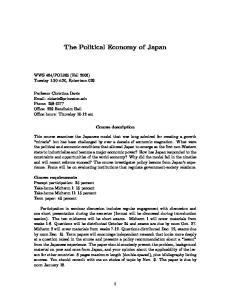
2005; Malmendier, 2009). Impressively, Rajan and Zingales (2003) assemble data on several indicators of financial development for a broad panel of countries. The authors observe that many Civil law countries, such as Austria, Belgium, and France, had a very high level of capital market development in the early twentieth century, even higher than the United States. They also identify structural breaks and, in particular, “Great Reversals” in many countries’ financial structure. Rajan and Zingales (2003) show that the reliance on capital markets of many Civil law countries shrank dramatically in the interwar period, while, at the same time, their governance mode shifted towards banks and other institutions at the expense of capital markets. Figure 1.1 illustrates well these Great Reversals. This figure presents yearly stock market capitalization data over the entire history of Belgium. Rajan and Zingales (2003) argue that these empirical patterns correlate with the role of dominant economic elites holding back financial development. In particular, the Great Reversals reflected a change, resulting from the Great Depression, in the ability of dominant elites to capture financial and product market regulations. However, the political explanation provided by Rajan and Zingales (2003) does not lend to fully account for the reasons why some Civil law countries, such as the Netherlands and Switzerland, maintained a market-oriented financial system. Indeed, the authors support the idea that the governance system in Civil law countries is more centralized and, thereby, easier for small elites to capture it.

Figure 1.1: The Historical Evolution of Belgian Stock Markets This graph shows the evolution of stock market capitalization ratio, which is the ratio of the market value of equity of domestic companies to GDP, in Belgium (1835-2009). Source: SCOB Database.

Chapter 1. General Introduction

6

Perotti and von Thadden (2006) argue in turn that major shocks hit asymmetrically countries in Continental Europe. In particular, Austria, Belgium, Germany, France, and Italy experienced large inflationary shocks after the World War One, while other countries do not. The authors offer a median voter model to predict that these price shocks impoverished the middle class, shaping its political preferences over the role of capital markets in society, and contributed to the Great Reversals. Perotti and von Thadden’s (2006) model is a key contribution as it allows to explain why some Civil law countries have not experienced further market development in the postwar period (see the case of Belgium in Figure 1.1), contrasting with other Civil law countries such as the Netherlands and Switzerland. Perotti and Schwienbacher (2009) propose an empirical test of this view, but they do not look directly at financial development. They show that large shocks in wealth distribution through hyperinflation in the interwar period explain the emergence of different structures of pension system in democratic countries. To explain differing contracting institutions and financial systems, related papers emphasize that not all institutions are equally difficult to change. One view also holds that political institutions are more difficult to change than legal institutions, and more broadly contracting institutions, and that for this reason political institutions have a substantial impact on contracting institutions and hence on the development of financial systems. Pagano and Volpin (2005) argue that some constitutional features affect contracting institutions. The authors predict that the electoral rule, by determining the formation of party coalitions representing specific groups of corporate stakeholders, influences the level of both shareholder and employment protection. They consistently show cross-country evidence that strong shareholder protection is more likely in countries with majoritarian electoral rule, while strong employment protection is more likely ˇ c´ık (2012) proposes a political economic in countries with proportional electoral rule. Sevˇ theory of the level of investor protection in a dynamic framework and endogenizes, in contrast, the proportion of each group of corporate stakeholders in the economy.8 In an early survey, Pagano and Volpin (2001) report that similar dynamics are at play for various financial policy measures, including bankruptcy, takeover, privatization, bailouts, branching restrictions, deposit insurance, and securities market. For example, Bergl¨of and Rosenthal (2000) explore the degree to which the populist and other debtor movements in the United States influenced the variation in bankruptcy laws over time. Biais and Perotti (2002) show how a conservative policy maker seeking reelection may design 8

In a subsequent paper, Pagano and Volpin (2006) study investor protection and stock market development in a political economy model and show that reinforcing feedback loops are at play generating multiple equilibria: Strong investor protection induces companies to issue more equity, increasing stock market size, which in turn may expand the investor base and increases support for investor protection. They show, consistently with their model, that international convergence in legal protection of outside investors is positively associated with cross-border mergers and acquisitions activity.

Chapter 1. General Introduction

7

privatization policies in such a way as to promote diffused financial shareholdings and align the preferences of the voters against redistributive policies. Caselli and Gennaioli (2008) analyze the different political feasibility of economic and financial reforms. Second, another strand of the political economy literature demonstrates that political institutions directly influence financial and economic development—with or without law. In their work, Engerman and Sokoloff (1997) shed light on the type of institutions arising during the colonial era in the New World and persisting over time. The emergence of differing institutions is due to initial conditions faced by New World colonial societies established by the Europeans—their respective factor endowments—that fostered equality or inequality. The authors provide detailed evidence that factor endowments such as climate, geography, natural resources, or soil conditions help explain long-run economic success of some countries through their impacts on institutions. Acemoglu, Johnson, and Robinson (2001) exploit empirically this argument and propose an analysis complementary to this story by arguing that the effect on institutions was the result of the mode of Western European settlement around the world. The mode of settlement can be divided into two broad categories that are related to factor endowments: those where Western Europeans had little interest in settling due to harsher and unfavorable conditions. In these colonies, mostly in Central America, the Caribbean, South Asia, or Africa, Western European settlers conquered and exploited natural resources without the concern to leave behind them favorable political institutions, which turned out to be harmful for subsequent economic growth and prosperity; and those, like in Australia or the United States, where Western Europeans settled in larger numbers and therefore developed political institutions more defensive of private property and of system of checks and balances in government. Acemoglu, Johnson, and Robinson (2002) show, in a companion paper, a similar effect of indigenous population density. They document that the regions of the world that were relatively rich around 1500 underwent a “reversal of fortune” subsequently. They argue that this militates against a geographic determinist view of development but the natural explanation for the reversal comes from the political institutions hypothesis. Another example of the direct role played by politics has to be found in the differing degrees of wartime destruction. One such argument is offered by Roe (2003, 2006), who argues that war damage shaped ownership structures and reliance on stock markets in richer countries, as a result of private choices. Countries that suffered from military invasion and occupation in the twentieth century overwhelmingly had Civil law legal systems, while no core English Common law countries collapsed or suffered similarly

Chapter 1. General Introduction

8

from both wars. The wars destroyed institutions, wrecked societal foundations, and ultimately shifted voters’ risk aversion and ideology.9 In Civil law countries that had nicely developed financial markets in 1913, war devastation made these countries indifferent or even antagonistic towards stock markets in the subsequent decades. Moreover, in an ideologically polarized context, the concentration of control in Continental Europe resulted from the need for corporate owners to counter the influence of organized labor. Summing up, Roe (2006: 498—499) writes: “I suspect it’s no accident that Switzerland—a civil law nation—has securities markets and ownership separation numbers that more closely resemble those in America and Britain than those in France or Germany: Switzerland is one of the few core civil law nations not destroyed during the twentieth century.” Even more directly, Acemoglu and Johnson (2005) evaluate the importance of legal versus political institutions in explaining cross-country differences in financial and economic development. They use well-known indicators in the political economy literature sourced from Polity IV and Political Risk Services to measure the political institutions of a society, that is, those constraining the expropriation by government and powerful elite (the authors coined instead the term “property rights institutions”). Employing instrumental variables strategies, their study reveals that political institutions have a first-order impact on long-run economic growth, investment, and the overall level of financial development (stock markets and the banking sector), while legal institutions—enabling private contracts between individuals—only appear to matter for stock market development. Their interpretation for these findings is as follows. Private agreements or reputation-based mechanisms can compensate for legal institutions, but alternative arrangements cannot compensate political institutions against the risk of expropriation. For example, banks can increase interest rates, provide closer monitoring, or develop reputation-based credit relationships, when it is more difficult for them to collect on their loans. Modigliani and Perotti (2000) show in this respect that bank-based financial system emerges in weak legal environment as banks are bound by some form of private enforcement. The effect of legal institutions is therefore limited given these possible alternative private arrangements. In contrast, when there is little protection for private property or few checks and balances against government expropriation, individuals do not have the conditions necessary for investment and trade. In this case, individuals are also unable to write credible contracts with the state to prevent future expropriation as the state is the ultimate arbiter of contracts. Beck, Demirg¨ u¸c-Kunt, and Levine (2003) undertake similar horse races between legal institutions and political institutions. They report that factor endowments (proxying political institutions) predict stock market and 9 Consistently, Perotti and Schwienbacher (2009) document that countries experienced sudden price shocks due to war damage show higher uncertainty aversion.

Chapter 1. General Introduction

9

banking development, whereas legal origins (proxying legal institutions) have little (or any) explanatory power, in line with the findings of Acemoglu and his co-authors.10 The literature on the political economy of finance is still fairly novel, but this brief introduction through the lens of the literature on comparative financial systems—of which this dissertation mostly belongs—demonstrates its impact and importance.

1.2

Political Economy in Finance: A Roadmap

As illustrated, the political economy approach, by pooling contributions from historians, political scientists, and economists, illuminates many important themes in finance. This dissertation has accordingly the following basic question as an overarching theme: What are the consequences of countries’ political system on their financial markets and intermediaries? It proceeds in answering this question along with the following theoretical framework derived from Acemoglu, Johnson, and Robinson (2005). This framework, though abstract and rather simple, serves as a guide for the three essays of this dissertation and, ultimately, enables to provide some answers to this basic question. A schematic representation of the framework is shown in Figure 1.2.

Figure 1.2: Causal Schema

As discussed in the previous section, differences in contracting and economic institutions, by shaping economic incentives, are a major source of cross-country differences in financial and economic development (the boxes on the right-hand side of Figure 1.2).11 These institutions determine the size of the aggregate pie, but also how the pie is divided among 10

Another closely related literature in political science and economics investigates the link between democracy and economic development (see, e.g., Papaioannou and Siourounis, 2008; Acemoglu, Naidu, Restrepo, and Robinson, 2014). Quintyn and Verdier (2010) show in a large sample of countries that sustained financial deepening is most likely to occur in stable democracies. 11 Acemoglu, Johnson, and Robinson (2005: 395) define good economic institutions as: “those that provide security of property rights and relatively equal access to economic resources to a broad crosssection of society.”

Chapter 1. General Introduction

10

different groups and individuals in society—i.e., the distribution of resources (physical capital, financial capital, and human capital). Contracting and economic institutions are however endogenous and determined by the distribution of political power. As differing contracting and economic institutions lead to variations in the distributions of resources, there is no guarantee that all individuals and groups have the same preferences regarding these institutions. Conflict of interests thus emerges among these individuals and groups. The prevailing equilibrium set of contracting and economic institutions is determined by their relative political power; that is, the institutions securing the best the interests of the groups or individuals that succeeded in asserting (politically) their wishes. In many cases this equilibrium can be costly for the society at large. In the finance literature, a bunch of theoretical papers shows that elites use their political power to pursue weak legal protection of outside investors as an indirect way to increase entry costs and thus avoid competition (Rajan and Zingales, 2003; Perotti and Volpin, 2007; Fulghieri and Suominen, 2012; Buck and Hildebrand, 2014). On the empirical side, much recent evidence shows that elites can restrict financial development in order to limit access to finance: Braun and Raddatz (2008) find that change in the strength of incumbent industries resulting from trade liberalization in 41 countries is a good predictor of subsequent financial development. Fogel, Morck, and Yeung (2008) show evidence that countries where the same companies maintain a dominant position over time have lower economic growth, weak investor protections, and less developed capital markets. Rajan and Ramcharan (2011) find that, in the 1920s, U.S. counties in which the agricultural elites have disproportionately large land holdings tend to have fewer banks per capita, costlier credit, and limited access to credit. Other empirical evidence shows how political connections create distortions in the allocation of capital and access to finance in developing and developed economies (see, e.g., Sapienza, 2004; Dinc, 2005; Khwaja and Mian, 2005; Claessens, Feijen, and Laeven, 2006; Duchin and Sosuyra, 2012; Behn, Haselmann, Kick, and Vig, 2014).12 Moreover, Acemoglu, Johnson, and Robinson (2005) offer a useful distinction between de jure and de facto political power. On one hand, de jure political power refers to power that originates from the political institutions (e.g., which segments of the population are enfranchised, how power is contested, how constrained the power of politicians 12

Another strand of this literature measures the value of political connections in countries with weak institutions such as Indonesia and Malaysia (Fisman, 2001; Johnson and Mitton, 2003) as well as in countries endowed with good institutions such as the United States (e.g., Cooper, Gulen, and Ovtchinnikov, 2009; Goldman, Rocholl, and So, 2009; Akey, 2013; Acemoglu, Johnson, Kermani, Kwak, and Mitton, 2013).

Chapter 1. General Introduction

11

and elites is, etc.).13 On the other hand, de facto political power is the political power that is not allocated by political institutions, but rather is possessed by individuals and groups as a result of their ability to organize, to use paramilitary forces and other means of repression, to lobby or bribe politicians, to capture and control political parties, etc. Figure 1.2 emphasizes in turn that the distribution of political power in society is endogenous: De jure political power is endogenous to political institutions, while de facto political power is endogenous to the distribution of resources. Political institutions and the distribution of resources are the fundamental variables in this framework because they change relatively slowly, and they determine directly and indirectly contracting/economic institutions and financial/economic development (see the previous section). Crucially, this theoretical framework is not static, political institutions, though highly persistent, are endogenous to de jure and de facto political power. The distribution of resources shapes incentives and preferences over outcomes and thus feeds back into de facto political power (the arrow at the bottom in Figure 1.2), which may lead to institutional political change. As an example, the emergence and flourishing of democracies across history have been characterized by the extent to which individuals were able to organize and engage in collective action to push for regime changes such as the presence of labor unions during the first wave of democratization in Europe prior World War One, or more recently the events of the Arab Spring helped with the massive use of social networks. Besides, those who hold de jure power can also influence political institutions by exercising their de jure power, and opt to maintain political institutions favorable to their interests.14 This theoretical framework thus emphasizes for potential changes of political institutions. These institutional political changes can be simply changes in the way political institutions function—such as Italy who abandoned its former reliance on full proportional representation in the 1990s, or the Belgian parliament which approved in 1993 the transformation of the country into a full-fledged federal state—but they can be far more discontinuous in the face of shocks. World history is plenty of examples of such discontinuous institutional political changes such as episodes of democratization, diffusion of political rights across the population, repression of different groups. A prominent 13 The label “political institutions” can be understood broadly—including, for example, social norms—but this label is here attached to formal rules, typically laid down by explicit provisions in constitutions (e.g., electoral and legislative rules associated with the forms of government), which entail different combinations of desirable attributes of a political system—namely, its accountability and representativeness. 14 Conflicts between de jure and de facto political power can be at play. For example, the transition from nondemocracy to democracy increases de jure political power, but at the same times elites may intensify their investments in de facto political power, for example via lobbying, in order to (partially) offset their loss of de jure political power (see Acemoglu and Robinson, 2008, for a formalization of this idea).

Chapter 1. General Introduction

12

example is the economic consequences of the evolution of the constitutional arrangements in the seventeenth century England following the Glorious Revolution of 1688 described in North and Weingast’s (1989) classical work. Later the French Revolution also produced a violent shock to the so-called Ancien R´egime, ending the reign of the absolutist French monarchs. On August 4, 1789, the National Constituent Assembly entirely changed French laws by proposing a new constitution which abolished the feudal system with the privileges it entailed and stated most notably equality before the law for all, not only in daily life and business, but also in politics. Decades of instability and war followed the French Revolution, but a slow and interrupted process ended French absolutism and led to the emergence of inclusive political and economic institutions, culminating in the Third Republic in 1870. Then, the French Revolutionary Armies and later Napoleon invaded large parts of Continental Europe, destroying absolutism, abolishing guilds, ending feudal land relations, and imposing the equality before the law. The French Revolution set in train a slow political emancipation of poorer classes not only in France but in much of the rest of Continental Europe. Furthermore, in the late nineteenth and early twentieth centuries, elites in many parts of Europe, in face of heightened social unrest (de facto power), were forced to grant suffrage to broader segments of the population. The broadening of suffrage is identified as an important factor in improving access to credit, reducing the power of monopolies, and promoting more intermediated finance (see Calomiris and Haber, 2014, for several case studies and Chapter 2 for a systematic analysis). This theoretical framework to finance-related issues makes up a rich research agenda, which is covered in the next three chapters of this dissertation. In particular, this dissertation offers three essays, each opening one box on the left-hand side of Figure 1.2, with financial markets and intermediaries as a common theme: The first essay focuses on political institutions (namely, the ones governing suffrage), the second one looks at de jure political power (namely, the type and composition of governments), while the third essay deals with de facto political power (namely, bank lobbying activities).

1.3

Outline of the Dissertation

Each of the three essays is a stand-alone contribution and can be read independently of the other essays. This dissertation is organized as follows. Chapter 2 contains a co-authored study analyzing how political institutions governing the expansion of suffrage impact on the historical evolution of countries’ reliance on both stock market and bank finance. By exploiting significant variation reflecting various suffrage restrictions between and within countries over the last two centuries, this study demonstrates that

Chapter 1. General Introduction

13

a political support for stock markets was possible when voting rights were limited to wealthy elites; consistent with the insight that narrow elites pursue economic opportunities by promoting capital raised on stock markets. In contrast, a political support for the banking sector emerges when voting rights spread across the population. Indeed, the expansion of suffrage induces a poorer median voter which has any (lower) financial holdings and, therefore, benefits less from the riskiness and financial returns from stock markets. A broader political participation empowers a middle class with different preferences, where banks are favored over stock markets since banks share its aversion to risk. This study consistently reports panel data evidence that countries with tighter suffrage restrictions tend to rely more on stock markets, whereas countries with broader suffrage are more conducive towards the banking sector. As a result, it finds evidence indicating that countries with tighter restrictions on voting franchise tend to have a more market-oriented financial system. The results presented are robust to controlling for other institutional arrangements, alternative hypotheses, and endogeneity. Chapter 3 presents a co-authored study examining the political outcomes driving the pace and extent of reforms aimed at supporting financial sector development. The last three decades of the twentieth century have been characterized by a global drive to reform finance, but progress has not been homogeneous. This chapter investigates the role of government cohesiveness in explaining part of this heterogeneity across countries and over time, finding that fragmented governments do breed stalemate. This phenomenon has often been assumed in the literature, based on circumstantial observations, but a formal, systematic assessment was still lacking. This study fills this gap by exploiting a panel dataset covering the OECD countries for 30 years and undertaking several robustness checks. It is worth emphasizing that this study controls for but does not concentrate on constitutional features—such as the electoral rule as in Pagano and Volpin (2005). It rather looks at political outcomes (the type of de jure political power) resulting from constitutional features, namely government fragmentation. Indeed, majoritarian electoral rules are more likely to produce single-party government, whereas coalition governments are more likely under proportional electoral rules. This study highlights that these political outcomes produce, as discussed in the previous section, systematic effects on financial policymaking, creating an indirect link between constitutional features and financial policy outcomes of interest. Chapter 3 also outlines three non-mutually exclusive theoretical mechanisms to explain the results: the first based on a war of attrition among political parties, the second on conflict of interests between constituencies, and the third on the possibility of lobbying individual members of a coalition. Chapter 4 shifts attention to the examination of the incidence and drivers of lobbying efforts made by the banking industry in the United States. This last study documents the relationships between lobbying, regulatory oversight, and bank risk taking. Using

Chapter 1. General Introduction

14

a large sample of commercial and savings banks, it finds that lobbying banks are less likely to be subject to a severe enforcement action, a key tool of banking micro-prudential supervision. These results suggest that banks engage in lobbying to gain preferential treatment. Among the lobbying dimensions studied, lobbyists with prior employment in public offices are more effective at reducing the probability of an action, especially in period of intense enforcement activity. These findings are robust to controlling for supervisory ratings and account for endogeneity concerns by employing instrumental variables strategies. This study also shows an increase in default and credit risk at lobbying banks. Overall, these results appear rather inconsistent with an informationbased explanation of bank lobbying, but consistent with the capture theory of regulation `a la Stigler (1971) and Peltzman (1976).

Chapter 2

Suffrage Institutions and Financial Systems∗ 2.1

Introduction

The quality of institutions is viewed as a fundamental determinant of economic growth and development through factor accumulation (North and Thomas, 1973; see Acemoglu, Johnson, and Robinson, 2005, for a review). In North and Thomas’s view, factor accumulation—including financial capital—is a proximate cause of growth. The fundamental explanation of comparative financial systems is thus differences in key institutional arrangements that define rules and rights aimed at protecting investors and ∗ This chapter is based on CEPR Discussion Paper No. 9621, “The Political Economy of Financial Systems: Evidence from Suffrage Reforms in the Last Two Centuries”, co-authored with Hans Degryse (Katholieke Universiteit Leuven) and Armin Schwienbacher (co-supervisor of this thesis). We are grateful to Senay Agca, Albert Banal-Estanol, Marco Becht, Thorsten Beck, Paul Belleflamme, Helen Bollaert, Fabio Braggion, Martin Brown, Micael Castanheira, Peter Cziraki, Narly Dwarkasing, Philip Fliers, Steve Haber, Iftekhar Hasan, Tarek Hassan, Sean Hundtofte, Filippo Ippolito, Ross Levine, Alessandro Lizzeri, Humberto Llavador, Ron Masulis, Raoul Minetti, Kris Mitchener, Steven Ongena, Kim Oosterlinck, Enrico Perotti, Thomas Piketty, Marco da Rin, Richard Roll, Henri Servaes, Elu von Thadden, John Turner, Paolo Volpin, Harald Uhlig, Burcin Yurtoglu, and Alberto Zazzaro for many helpful discussions. We have also benefited from the comments of seminar participants at the Universities of Antwerp, Bangor, Bologna, Ghent, Louvain, Munich, Pompeu Fabra, Queen’s Belfast, Tilburg, London Business School, Paris School of Economics, SKEMA Business School, WHU School of Management, and participants at the 2012 NBB-3L Finance Workshop (Brussels), the 2013 MoFiR Workshop on Banking (Ancona), the 2013 ECORE Workshop on Governance and Economic Behavior (Leuven), the 2013 EEA Meetings (Gothenburg), the 2013 FMA Meetings (Chicago), the 2013 Surrey-Fordham Banking Conference (Guildford), the 2013 CESifo Workshop on Political Economy (Dresden), the 2013 HEC Paris Workshop on Finance and the Real Economy (Jouy-en-Josas), the 2014 ECCCS Workshop on Governance and Corporate Control (Lille), the 2014 ALEA Meetings (Chicago), the 2014 Belgian Financial Research Forum (Louvain-la-Neuve), the 2014 EFA Meetings (Lugano), the 2014 Corporate Finance Day (Paris), the 2014 EBC-CEPR Financial Stability Conference (Tilburg), and the 2015 AEA Meetings (Boston).

15

Chapter 2. Suffrage Institutions and Financial Systems

16

supporting private contracts.1 Three fundamental institutions are critical for financial rules and rights, and hence for the development of financial systems: legal, cultural, and political institutions (La Porta, Lopez-de-Silanes, Shleifer, and Vishny, 1998; Rajan and Zingales, 2003; Stulz and Williamson, 2003; Acemoglu and Johnson, 2005). Fundamental institutions, such as legal origins and persistent cultural traits, are clearly important and there is convincing evidence confirming their roles for the development of financial systems.2 However, they do not lend to fully account for time-series variation in financial systems as changes in legal origin or culture are extremely rare. They therefore ought to be complemented by other institutional views. Of primary importance to explain the rise and decline of stock markets and banking sector is the evolution in political institutions, as acknowledged by Haber, North, and Weingast (2007); in particular, political institutions governing the expansion of suffrage,3 a key measure of the distribution of political power. Notwithstanding that economic historians have argued that political institutions shaped financial systems, there has been little systematic examination of the evidence, especially from an international perspective. This paper empirically examines how the diffusion of voting rights across the population helps to explain the historical evolution in a country’s reliance on both stock market and bank finance.4 We focus on the scale of external finance (hereafter, financial development) but also on the degree to which countries have bank-based or market-based financial systems (hereafter, financial structure) (see, e.g., Beck and Levine, 2002). Financial development and structure have been conclusively shown in the literature to accelerate economic growth (for a review see, e.g., ESRB, 2014). Suffrage reforms during the late nineteenth and the twentieth centuries are crucial political changes. Suffrage reforms affect the ability of elites to obtain disproportionate political leverage, and to design legal frameworks and state policies to benefit themselves relative to others in terms of access to finance and economic opportunities. Paying attention to changes in suffrage institutions gives indeed insights into the shifts in political equilibria affecting financial systems over time. For example, Benmelech and Moskowitz 1

There is ample evidence showing that rules and rights aimed at protecting outside investors, including minority shareholders and creditors, and supporting private contractual arrangements do matter for the development of financial systems; see, e.g., La Porta, Lopez-de-Silanes, Shleifer, and Vishny (1997, 1998), Levine (1998), Modigliani and Perotti (2000), La Porta, Lopez-de-Silanes, and Shleifer (2006), or Djankov, McLiesh, and Shleifer (2007). 2 See La Porta, Lopez-de-Silanes, and Shleifer (2008) who review the theory and empirical findings of legal origins. On the role of culture, see most notably Stulz and Williamson (2003), Guiso, Sapienza, and Zingales (2004a), Licht, Goldschmidt, and Schwartz (2005), and Siegel, Licht, and Schwartz (2011). 3 We use the terms “suffrage” and “franchise” interchangeably throughout the paper. 4 Our study builds on the seminal work by Rajan and Zingales (2003), Roe (2003), Gourevitch and Shinn (2005), Perotti and von Thadden (2006), Haber, North, and Weingast (2007), Malmendier (2009), Roe and Siegel (2009), Calomiris and Haber (2014), and many others who conceive historical changes in a country’s financial system as reflecting shifts in the distribution of political power. Perotti (2014) provides an excellent survey on the political economy underpinnings of financial systems.

Chapter 2. Suffrage Institutions and Financial Systems

17

(2010) show that financial regulation was exploited by elites with political power for their own interests in nineteenth century America. They provide evidence that usury laws—limiting the maximum legal interest rates—were used to hamper competition and control entry. States that restricted suffrage to taxpaying property owners tended to impose more strict usury laws.5 Haber (2011) documents for Brazil, Mexico, and the United States that less inclusive suffrage institutions amplified the political power of elites and that their power inhibited policies governing banks, which in turn shaped the size and competitive structure of the banking sector (see also Calomiris and Haber, 2014). Using stock price data, Turner and Zhan (2012) find that investors in British firms, foreseeing future alterations of their property rights, responded negatively to the 1867 suffrage reform. As illustrated, the prevalence of inclusive suffrage institutions and constraints on elites’ political power facilitate access to credit and promote more intermediated (bank) finance (see also Barth, Caprio, and Levine, 2006).6 While broader voting rights lead to higher level of financial development, financial structure can still differ markedly across democracies. Rajan and Zingales (2003) actually observe significant cross-country differences in financial structure. The authors also document rapid changes occurring in financial structure during the twentieth century and identify in particular “Great Reversals” experienced by many European countries in the interwar period and Japan after the Second World War. Embedded in the premise underlying interest group theory of suffrage institutions (Engerman and Sokoloff, 2005), our paper goes beyond narrative insights and countryspecific studies and investigates whether the impact of suffrage institutions on financial development and structure is generalizable to a broad set of countries. Combining various data sources, we construct a unique historical panel dataset allowing us to provide external validity regarding the all-important question of the link between suffrage and both stock market and bank finance.7 This allows us to exploit important variation in suffrage institutions in a time series and cross-sectional dimension and draw more general conclusions on the political economy underpinnings of financial structure. The main analysis relies on a panel dataset of 18 today’s established democracies covering the nineteenth and twentieth centuries and for which we obtained sufficiently reliable data. 5

Relatedly, Bolton and Rosenthal (2002) give a theoretical explanation for why U.S. states with less inclusive suffrage institutions were less likely to pass debtor relief legislation. 6 Focusing on the banking sector, Quintyn and Verdier (2010) relatedly show in a large sample of countries since the early 1960 that sustained financial deepening is most likely to occur in countries endowed with high-quality political institutions. Bordo and Rousseau (2006) find similar evidence in a more historical perspective. 7 In Haber’s (2011) conclusion, the question of external validity of the link between suffrage institutions and banking development is raised as follows: “Are these results generalizable? Obviously, more detailed case studies beyond the three presented here [i.e., Brazil, Mexico, and the United States] are necessary before any firm conclusions should be draw [. . . ]”.

Chapter 2. Suffrage Institutions and Financial Systems

18

While our sample only includes 18 countries, it represents almost the entire population of countries with a history of democratic voting. Summary statistics depict significant variation between and within countries reflecting various suffrage restrictions based on wealth, social status, education, gender, and race. More specifically, summary statistics indicate that voting franchise was low at the beginning of the twentieth century, with on average 17.3% of the population allowed to vote in 1900. This percentage increased to 25.5% around 1913 and crossed the 50% mark generally after the Second World War only. Exploiting these variations using standard panel data techniques, we show evidence that suffrage institutions have a strong economic and statistical effect on financial development and structure. Countries with tighter restrictions on their voting franchise tend to rely more on stock markets, whereas countries with broader voting franchise are more conducive towards the banking sector, reflecting the political support of the newly enfranchised segment of the population. Employing our most conservative estimates, a one standard deviation greater voting franchise leads to a 24.6% lower degree of stock market capitalization and a 16.1% greater banking sector development. As a result, we do find evidence indicating that countries with tighter restrictions on voting franchise tend to have a more market-oriented financial structure. Our findings are consistent with the insight that narrow elites pursue economic opportunities by promoting capital raised on stock markets. In contrast, a broader political participation empowers a middle class with different preferences, where banks are favored by limiting the rights of minority shareholders. Bank finance is preferred by less financially wealthy citizens with proportionally more exposure to labor income, as it contains corporate risk. This prediction arises as a median voter equilibrium in Perotti and von Thadden (2006), but a similar implication arises when government formation depends on interest group coalitions (Pagano and Volpin, 2005; see also Hellwig, 2000; and Gourevitch and Shinn, 2005). By moving (the location of) the median voter or by determining the ruling coalition, the scope of the voting franchise directly influences the development and structure of a country’s financial system. We also address the cross-sectional implications of several complementary hypotheses related to other (observable and unobservable) factors of institutional quality affecting financial development and structure. First, we control for observable factors such as legal origins, religious composition, and electoral rules, among other institutional arrangements. Second, the respective contribution of each of these fundamental institutions is hard to disentangle, as it is in part a matter of definitions and of indicators construction (Glaeser, La Porta, Lopez-de-Silanes, and Shleifer, 2004; Acemoglu and

Chapter 2. Suffrage Institutions and Financial Systems

19

Johnson, 2005).8 We overcome, however, objections related to other unobservable factors of institutional quality in the following ways. We include country fixed effects in our specifications in order to remove the effect on financial outcomes of fixed country characteristics potentially correlated with suffrage. We also include year fixed effects to remove any common global trends in suffrage that may be correlated with financial outcomes. Critically, our results hold even after controlling for GDP per capita and wealth inequality. We further address potential concerns about omitted variable bias by adopting a difference-in-differences (DID) approach. This allows us to exploit exogenous inter-temporal variations from two major suffrage reforms across countries— namely, male and female universal suffrage reforms. The DID methodology confirms our predictions. All in all, in these efforts to unbundle institutions, the economic and statistical significance of suffrage institutions are unaffected. Our results also contrast with the time-series implications of the “modernization hypothesis”. The central tenet of the modernization hypothesis as articulated by Lipset (1959) is that economic development causes a country to be democratic. This would suggest that our results do not establish causality and that they are driven by reverse causality. Reverse causality cannot be ruled out easily, since expansion of the voting franchise can be the result of economic growth and factor accumulation, rather than a cause thereof. Although the most recent studies give little empirical support for the modernization hypothesis (see, e.g., Acemoglu, Johnson, Robinson, and Yared, 2008, 2009; Aidt and Jensen, 2014), we further use an instrumental variables (IV) approach to mitigate concerns about the cause-and-effect relationships involved. We employ proper instruments that are country-time level varying by building on the historical and theoretical literature on the reasons why governing elites granted suffrage to other segments of the population. Using this IV strategy, we obtain results confirming the predictions of a link going from suffrage institutions to financial development and structure. Finally, we investigate whether suffrage institutions exert long-run effects. We find that the time of adopting universal suffrage has long-lasting impacts on financial structure. Extending the set of countries to 35, our long-run evidence reveals an impressive impact of the delayed introduction of the universal suffrage on the form of today’s financial systems: a 25-year delay in the introduction of universal suffrage relates to a remarkable 17.5% increase in the today’s importance of stock markets relative to the banking sector. 8

Indeed, there can be big overlap between legal systems, religious composition, and national political institutions making it hard to isolate the idiosyncratic component of these features (especially working with small samples of countries). For example, judicial review can be equally seen as a legal or a political institution limiting government discretion, while enforcement of contracts requires legal rules as well as government support. Also, legal origin may proxy for institutions that are not fundamentally related to the legal systems: Common law countries are primarily Protestant, while French civil law countries are overwhelmingly Catholic. The legal origin view has evolved over time as argued by La Porta, Lopezde-Silanes, and Shleifer (2008). Now the authors seem to adopt a more cultural interpretation of legal origin “as a style of social control of economic life”.

Chapter 2. Suffrage Institutions and Financial Systems

20

Our paper contributes to the literature in the following ways. First, supporting evidence on the political institutions view has been primarily based on panel studies across U.S. states (Benmelech and Moskowitz, 2010; Rajan and Ramcharan, 2011), or crosssectional variation around significant historical discontinuities, such as the Great Reversals (Rajan and Zingales, 2003; Perotti and Schwienbacher, 2009). This paper goes beyond by assembling a broad historical panel of countries and identifying evidence for the new generation of political economy models (Pagano and Volpin, 2005; Perotti and von Thadden, 2006). We add in turn to this new generation of political economy models by stressing the role played by suffrage institutions. Second, this paper empirically shows how broadening the electorate affects not just the scale of external finance over time but also its structure. This result allows to distinguish their effects from complementary hypotheses such as the legal origin view (La Porta, Lopez-de-Silanes, Shleifer, and Vishny, 1997, 1998) or the majoritarian/proportional view of government policies (Persson and Tabellini, 2003; Pagano and Volpin, 2005). Indeed, Modigliani and Perotti (2000) suggest that in weak legal environments, banks may provide closer monitoring than dispersed shareholders. The legal origin view shows that banking is particularly developed in the German legal tradition. Even if some civil law traditions were systematically less supportive of shareholder rights, and banks represent the alternative, a (time-varying) political explanation was still lacking. We provide in this respect an empirical attempt showing why over time depositors would be better protected than shareholders. Third, our empirical setting illuminates causality, running from suffrage institutions to financial outcomes, and thus offers evidence for a richer alternative to a simplistic modernization hypothesis. Finally, this paper speaks to the dominant political science literature centered on the “Varieties of Capitalism” model (Hall and Soskice, 2001), of which our evidence rationalizes the approach. The remainder of this paper is structured as follows. Section 2.2 develops the theoretical framework and testable hypotheses. Section 2.3 describes the data and proceeds with a discussion of initial assessments of our hypotheses. Section 2.4 contains our main empirical results, while the long-run analysis is presented in Section 2.5. Section 2.6 concludes.

2.2

The Suffrage and Finance Nexus

This section clarifies the channel through which suffrage institutions affect financial development and structure. In this way, we lay out the main hypotheses to be tested. We then provide some case studies to further illustrate the economic channel we capture.

Chapter 2. Suffrage Institutions and Financial Systems

2.2.1

21

Theoretical Framework and Testable Hypotheses

The premise underlying institutional quality arguments is that key institutional arrangements that define rules and rights are regarded as pre-conditions of the development of financial systems. In particular, the political institutions view considers that good political institutions should come first because they determine the distribution of political power in society: let people vote to influence their fortune, and to constrain elites from abusing power. In the tradition of classical political economy, we consider that financial rules and rights affecting financial systems are the result of political decision-making, which are in turn influenced by economic interests. As corporate stakeholders, voters have preferences about external financing because it affects corporate decisions, which drive the creation and distribution of national wealth. Suffrage institutions, by determining the enfranchised segments of the population, constitute therefore a corner stone of political outcomes. By voting for their representatives, the enfranchised population can influence the political agenda, and thus the implementation of policies protecting their interests. As shown, broadening the electorate is consequential as it undermines regulatory capture by elites, increases the access and provision of credit to the private sector (Bordo and Rousseau, 2006; Barth, Caprio, and Levine, 2006; Benmelech and Moskowitz, 2010), and helps protect property rights as well as investor rights (North and Weingast, 1989). The models of democratic choice—such as Pagano and Volpin (2005) and Perotti and von Thadden (2006)—predict that political preferences, which are determined by the distribution of equity ownership in the economy,9 shape the national financial system. In other words, in this view, voters’ preferences at each point in time determine the scale of stock markets and banking sector and thereby also the relative importance of stock markets vis-` a-vis the banking sector. We hypothesize that countries with tighter restrictions on voting franchise tend to have higher levels of stock market development. In contrast, countries with broader franchise tend to have higher levels of banking sector development. These two predictions follow Perotti and von Thadden’s (2006) median voter equilibrium.10 The political support for banks or stock markets is determined by the median voter, which has a mixed identity as investor and worker. If the median voter has little financial wealth and mainly relies on labor income, a political majority will favor high labor and creditor protection. Indeed, this median voter will assign a central role to banks 9

This assumption is consistent with empirical observations. For example, Kaustia, Kn¨ upfer, and Torstila (2014) empirically examine the role stock ownership plays in shaping political preferences and find a positive and economically significant effect on right-of-center vote share. 10 Biais and Mariotti (2009) take a similar theoretical setting to analyze the political process through which bankruptcy laws can emerge.

Chapter 2. Suffrage Institutions and Financial Systems

22

over stock markets since banks share its aversion to risk. Banks have a tendency to limit risk-taking behavior of corporate managers, since, as debtholders, they do not benefit from the upside potential of riskier investments. In contrast, if the median voter has sufficient financial wealth, a majority will support strong minority shareholder protection and therefore a greater role for stock markets. Stock market development results in riskier but more profitable investments at the cost of higher labor risk-bearing. Similar predictions arise from interest group coalition as in Pagano and Volpin (2005). In this theoretical setting, suffrage institutions play a key role since they affect the median voter. The expansion of the voting franchise, by adding voters that were drawn mostly from the lower end of the wealth distribution, allows switching political majorities towards the preferences of the newly enfranchised segment of the population.11 As an example, Morgan-Collins (2013) analyzes eleven European countries for the period 1888-1975 and shows that an increase in the size of enfranchised population resulted in an increased support for socialist parties. Thus, limited suffrage ensures power to a relatively wealthy median voter, favoring stock markets, whereas a broader suffrage moves the median voter towards lower income classes, favoring the banking sector.12 As discussed in the introduction 2.1, financial structure differs across countries, crosssectional as well as over time (Rajan and Zingales, 2003). In an early contribution, Modigliani and Perotti (2000) suggest that in an unreliable enforcement regime, transactions tend to become intermediated through banks, which are bound by some form of private enforcement. La Porta, Lopez-de-Silanes, Shleifer, and Vishny (1997, 1998) show evidence that banking sector development is higher in German civil law countries. Even if the rights of minority shareholders are on average weaker in some Civil law countries, and banks represent the alternative, political explanations of why creditors would be better secured than minority shareholders are still necessary. In this respect, the models of democratic choice (Pagano and Volpin, 2005; Perotti and von Thadden, 2006) are able to account for observed variation also across Civil law countries, while changes in suffrage institutions further account for observed variation over time. This results in our third prediction: Countries with tighter restrictions on voting franchise tend to have a more market-oriented financial structure. 11

Economic theory provides different channels leading political elites to broaden the voting franchise. According to Acemoglu and Robinson (2000, 2006), the expansion of the voting franchise can be understood as a rational response by the governing elites to avoid revolution. In contrast, Lizzeri and Persico (2004) and Llavador and Oxoby (2005) argue that the expansion of the voting franchise was the result of the divergence of interests existing within the elites. 12 In this respect, our study also complements another strand of the literature devoted to the economic effects of suffrage. This literature, echoing earlier concerns of Alexis de Tocqueville’s Democracy in America ([1835] 1965), largely associated the expansion of the franchise with increases in the size of government (e.g., Husted and Kenny, 1997; Justman and Gradstein, 1999; Aidt, Dutta, and Loukoianova, 2006).

Chapter 2. Suffrage Institutions and Financial Systems

2.2.2

23

Case Studies

A closer look at countries from different legal traditions—England, Belgium, and Sweden— offers valuable insights of many of the themes in the paper. The history of British banking after the Napoleonic Wars was not seamless and key changes in the distribution of political power are reflected in its evolution, as described in details by Calomiris and Haber (2014, chapters 4 and 5). In the eighteenth and early nineteenth centuries, elites in control of the government were not particularly concerned about government policies that target the ability of common people to get bank credit, leaving them in the cold. However, a series of gradual expansions of suffrage in the nineteenth century made small elites more and more powerless. The 1832, 1867, 1884 acts broke centuries of tradition by progressively reducing property requirements for the franchise and allowing several segments of the male population (comprising members of the working class) to vote.13 The period before 1860 signed the end of the Bank of England’s monopoly and saw the emergence of competing chartered banks, operating on a branching basis and serving the needs of private commerce and industry. By the end of the nineteenth century, the English banking system consolidated, by achieving stability and broadening credit provision. Consequently, for over a century after 1850, the English banking sector grew dramatically in terms of both deposits relative to GDP and borrowers’ access to banks or bank offices. About this period, Calomiris and Haber (2014: 128) add: “By 1904, there were over 15,000 branches of the Post Office Savings Bank and roughly 400 offices of trustee savings banks. These new institutions reflected the rise of the middle class as both an economic reality and a political force seeking its own sources of financing.” In the second half of the nineteenth century, Belgium passed several reforms on stock exchanges, while its franchise was fairly narrow.14 In 1867, government gave up its right to ban firms from trading on the stock exchange. The Company Reform Act of 1873 abolished in turn government approval to set up a limited liability firm. By embracing these reforms, the Brussels Stock Exchange experienced its fastest development. Van Nieuwerburgh, Buelens, and Cuyvers (2006: 26) uncover that “between 1873 and 1914, the total number of listed shares increased from 174 to 1197.” In the years after the First World War, Belgium witnessed a reversal of the reforms of 1867 and 1873. In 1919, plural voting is abolished and universal suffrage for men over 21 is introduced, increasing the representation of the Workers Party. The years following these suffrage 13

The 1832 “Great Reform” Act increased, for example, the political representation of the burgeoning industrial cities (like Birmingham and Manchester) at the expense of the so-called rotten boroughs (locations with minuscule populations). 14 Belgium had a restricted manhood suffrage till 1892 with high direct tax minima differing in urban and rural areas. Male universal suffrage, modified by plural voting, was introduced in 1893. Plural voting allows a maximum of 3 votes per person depending on education diploma, social status, or property ownership.

Chapter 2. Suffrage Institutions and Financial Systems

24

reforms are characterized by a massive concentration in the banking sector, stimulated by the law of July 23, 1927. Then, the regulatory reforms of the financial system in 19341935 tightened to a certain extent government control over the stock exchange. Various events of the era—such as distributional shocks and institutional political reforms—led the Belgian stock market development to reach its peak in 1929 and to drop off sharply afterwards. H¨ogfeldt (2005) describes how the expansion of voting franchise in Sweden generated institutional settings that affected the financial structure of the country. Until universal suffrage was introduced in 1921, the Swedish economy had a well-developed stock market, with a large fraction of the economy held by a few very rich families. The expansion of suffrage however secured long-lasting political power to the Social Democratic Party from 1932 onwards, creating the ground for a more egalitarian economy based on strong corporatism and less stock market development.

2.3

Data and Initial Assessments

We now introduce the dataset we use throughout our main analysis of the paper and present preliminary assessments of the link between suffrage institutions and financial development and structure. We document that countries with (1) tighter restrictions on voting franchise are conducive to higher levels of stock market development; (2) countries with broader voting franchise are conducive to higher levels of banking sector development; and in turn (3) countries with tighter restrictions on voting franchise tend to have a more market-oriented financial structure. To this end, Table 2.1 provides definitions of our variables and their sources, Table 2.2 contains descriptive statistics, and Table 2.3 depicts the evolution of suffrage institutions in our sample countries. Table 2.2 also provides tests of differences in suffrage institutions for low and high countries’ levels of financial development and structure as well as pairwise correlations between our financial and suffrage indicators.

2.3.1

The Sample

Time-series variation in voting franchise is important to capture its impact on financial development and structure. Our base sample employs an 18-country panel dataset which covers the longest time span possible, composed of different years spaced by around ten years. The analysis on stock market development covers the nineteenth and twentieth centuries while the analysis on banking sector development and financial structure is restricted to the twentieth century due to data availability. Our dataset comprises a

Chapter 2. Suffrage Institutions and Financial Systems

25

set of today’s established democracies for which we have sufficient information on stock markets, banking sector, suffrage institutions, and country-specific characteristics. The countries included in the panel dataset are reported in Table A.1 in Appendix A (in bold). We are dealing with an unbalanced panel (see Table 2.2). However, every country is well covered in the time-series dimension as the average number of observations for a country in the twentieth century is 9 (out of maximum of 10).

2.3.2

Indicators of Financial Development and Structure

We use indicators capturing the scale and the structure of external finance in a country over time. The goal is to proxy for the degree of availability of stock market finance and bank finance. We rely on a variety of indicators that are commonly used in the literature on comparative financial systems (see Beck, Demirg¨ uc¸-Kunt, and Levine, 2000). We employ two indicators for the size of a country’s stock market. The first is stock market capitalization to GDP (CAPITALIZATION). We combine several data sources to obtain the longest time series possible (1830-1999)—Goldsmith (1985), Rajan and Zingales (2003), and Musacchio (2010). We mainly rely on data provided by Rajan and Zingales (2003) where the stock market capitalization to GDP is covered from 1913 to 1999 and reported for 24 countries. Musacchio (2010) however proposes improved estimates for 1913 and complements it with 1900, as Sylla (2006) and La Porta, Lopezde-Silanes, and Shleifer (2008) had questioned the accuracy of Rajan and Zingales’s figures in 1913: the inclusion of corporate bonds and cross-listed companies produced poor estimates in 1913. We therefore employ the re-estimated data of Musacchio (2010) for the years 1900 and 1913 and the data of Rajan and Zingales (2003) for the following years. Goldsmith (1985) provides additional data on stock market capitalization to GDP for the nineteenth century but for fewer countries. We complete our dataset by using Goldsmith (1985) yielding us with observations going back to 1830. The second indicator of the size of the stock market is the number of publicly listed domestic companies per million of inhabitants (LISTED COMPANIES). This variable is less prone to fluctuation of stock valuations and is retrieved from Rajan and Zingales (2003), but is available for the period 1913-1999 only.15 BANK DEPOSITS is our indicator for the size of a country’s banking sector. It is defined as the ratio of commercial and savings deposits to GDP. While this indicator does not provide clear information about the amount of private credit granted by the banking sector, it is one of the few that has been compiled in a standardized manner for 15

We also complete the Rajan and Zingales’s series on stock market development for Belgium with data taken from the SCOB database maintained at the University of Antwerp. We thank the SCOB for providing these data.

Chapter 2. Suffrage Institutions and Financial Systems

26

Table 2.1: Description of Variables Variable

Description

Sources

Financial Development and Structure CAPITALIZATION

Stock market capitalization divided by GDP.

Rajan and Goldsmith Rajan and Rajan and Rajan and

LISTED COMPANIES BANK DEPOSITS STRUCTURE Suffrage Institutions SUFFRAGE

Number of publicly traded domestic companies per million of inhabitants. Deposits at commercial banks and savings banks divided by GDP. Ratio of stock market capitalization to bank deposits.

EFFECTIVE SUFFRAGE

The number of valid votes cast for the lower house of the national legislature divided by total population.

Controls GDP PER CAPITA URBANIZATION RATE LAND AREA LATITUDE COMMON LAW ORIGIN CATHOLIC POLITY 2

MAJORITARIAN RULE

TOP INCOME SHARE TRADE OPENNESS GOVERNMENT EXPENDITURE Instruments THREAT OF REVOLUTION

INTERNATIONAL NORMS

POPULATION GROWTH

The number of registered voters for the lower house of the national legislature divided by total population.

Per capita GDP (1990 international Geary-Khamis dollars). The proportion of the population that lives in cities with more than 100,000 inhabitants. Land area (sq. km). Absolute value of the latitude of a country, scaled between zero and one. Dummy variable equal to one for English common law legal tradition, and zero otherwise. Dummy variable equal to one if Catholic religion is the religion practiced by the largest fraction of the population, and zero otherwise. Dummy variable equal to one if “Polity2” is positive and zero if negative. Polity2 is an index summing a democracy score (ranging from 0 to 10) for each country and year with an autocracy score (ranging from 0 to -10), with higher values associated with better democracies. The former is an institutional measure of democracy based on country’s competitiveness and openness in selecting the executive, political participation, and constraints on the chief executive, whereas the latter scores autocratic limitations on the same dimensions of democratic rights. Dummy variable equal to one if the country elected its lower house exclusively through plurality rule in the most recent election, whereas for other (mixed and proportional) rules it equals zero. Top 1% income share. Income is defined as market income including capital gains (excludes all government transfers). Top 1% denotes the top percentile. The proportion of world trade (imports and exports). National government expenditure per capita. Index of the threat of revolution. It is a simple count of major revolutionary events occurring in neighboring countries in a given year. The index remains at its value in each year after the introduction of adult male suffrage. Proportion of countries around the world having introduced universal suffrage for all men and women. The measure remains at its value in each year after universal suffrage. 10-year average of the annual growth rate of the total population.

Zingales (2003), Musacchio (2010), (1985), and SCOB Database Zingales (2003) Zingales (2003) Zingales (2003), and Musacchio (2010)

Mackie and Rose (1982), Colomer (2001), Banks (2011), and International Institute for Democracy and Electoral Assistance (IDEA) Banks (2011)

Maddison (2003) Banks (2011) Banks (2011) La Porta, Lopez-de-Silanes, Shleifer, and Vishny (1999) La Porta, Lopez-de-Silanes, Shleifer, and Vishny (1999) Stulz and Williamson (2003) Polity IV Database

Flora (1983), Colomer (2001), and Persson and Tabellini (2003) The World Top Incomes Database Banks (2011) Banks (2011) Mackie and Rose (1982), Aidt and Jensen (2014), Banks (2011), and authors’ own calculations Ramirez, Soysal, and Shanahan (1997), and authors’ own calculations Banks (2011) and Maddison (2003)

Chapter 2. Suffrage Institutions and Financial Systems

27

a long time-series and for a large cross-section of countries and was employed before by Rajan and Zingales (2003).16 Finally, we also look at the orientation of the financial system by using a measure of the importance of stock markets as compared to the banking sector. We define STRUCTURE as the ratio of CAPITALIZATION to BANK DEPOSITS; if this indicator is greater than one, it means that in a given country the size of the stock market is larger than the size of the banking sector, thereby suggesting that the financial system is market-oriented. Some countries from the Rajan and Zingales’s (2003) dataset are not in our dataset since our concern is primarily the period covered before the Second World War and financial data available for this period are somewhat sparse. Our sample ends up being 18 countries over the time period of 1830-1999 for CAPITALIZATION and 1913 to 1999 for LISTED COMPANIES, BANK DEPOSITS, and STRUCTURE.17 The top part of Panel A in Table 2.2 reports the descriptive statistics for our indicators of financial development and structure—mean, standard deviation (overall), standard deviation (within), and standard deviation (between). The mean value of CAPITALIZATION is 0.576 and the within country standard deviation is 0.411. We also note substantial variation across countries in CAPITALIZATION with a between standard deviation of 0.319. This substantial variation between and within countries is confirmed using the other stock market development indicator, LISTED COMPANIES. Table 2.2 also indicates high variability between and within countries for our indicator of banking sector development, BANK DEPOSITS. Regarding financial structure, the average value of STRUCTURE is 2.041, indicating that on average countries in our sample have a market-based financial system. STRUCTURE varies quite a bit over time. As an illustration, in 1913, STRUCTURE identifies Spain and Japan (Norway and Austria) as having the most market-based (bank-based) financial systems. In contrast, the United States and the United Kingdom (Austria and Belgium) are classified as countries with the most market-based (bank-based) financial systems in 1999. 16

The BIS has recently made a panel dataset available on domestic bank credit to the non-financial sector (see http://www.bis.org/statistics/credtopriv/documentation.pdf). The dataset however does not cover the period before the Second World War. 17 Years under consideration are 1830, 1850, 1861, 1875, 1880, 1881, 1895, 1899, 1900, 1913, 1929, 1938, 1950, 1960, 1970, 1980, 1990, and 1999. Rajan and Zingales (2003) also employ the fraction of gross fixed-capital formation raised through equity issues. We do not use this indicator as it is not available for many countries and years under consideration before the Second World War.

28

Table 2.2: Descriptive Statistics, Tests of Differences, and Pairwise Correlations: Panel Data

Chapter 2. Suffrage Institutions and Financial Systems

This table presents descriptive statistics (Panel A), tests of differences (Panel B), and pairwise correlations (Panel C) for our 18-country panel dataset spanning from 1830 to 1999. Panel B tests the difference in means, for each indicator of suffrage institutions, between low and high countries’ levels of financial development (i.e., values below and above the median). Panel C reports pairwise correlation coefficients between our financial development indicators and suffrage indicators. Table 2.1 summarizes variables definitions and sources. *, **, and *** indicate significance at the 10%, 5%, and 1% levels, respectively. Panel A: Descriptive Statistics Std Dev Std Dev (Overall) (Between) Financial Development and Structure CAPITALIZATION 0.576 0.509 0.319 LISTED COMPANIES 34.215 27.103 21.109 BANK DEPOSITS 0.421 0.302 0.173 STRUCTURE 2.041 2.370 1.716 Suffrage Institutions SUFFRAGE 0.475 0.241 0.108 EFFECTIVE SUFFRAGE 0.377 0.202 0.120 Controls ln(GDP PER CAPITA) 1.814 0.790 0.308 URBANIZATION RATE 0.257 0.150 0.111 ln(LAND AREA) 5.936 1.768 1.822 LATITUDE 0.516 0.117 0.123 COMMON LAW ORIGIN 0.273 0.446 0.461 CATHOLIC 0.500 0.501 0.514 POLITY 2 0.874 0.333 0.150 MAJORITARIAN RULE 0.535 0.500 0.389 Variable

Mean

Std Dev (Within)

Nb of Countries

Nb of Obs

0.411 16.702 0.251 1.618

18 18 18 18

178 138 162 144

0.222 0.172

18 18

190 170

0.737 0.102 0.092 0.000 0.000 0.000 0.297 0.331

18 18 18 18 18 18 18 18

195 194 198 198 198 198 198 198 (continued )

SUFFRAGE EFFECTIVE SUFFRAGE SUFFRAGE EFFECTIVE SUFFRAGE SUFFRAGE EFFECTIVE SUFFRAGE

(1) (2) (3) (4) (5) (6)

ln(CAPITALIZATION) ln(LISTED COMPANIES) ln(BANK DEPOSITS) ln(STRUCTURE) SUFFRAGE EFFECTIVE SUFFRAGE

Test Diff. (p-value) 0.204 0.003 0.007 0.005 0.008 0.045 0.003 0.000 (5)

(6)

1.000 0.930***

1.000

Chapter 2. Suffrage Institutions and Financial Systems

SUFFRAGE EFFECTIVE SUFFRAGE

Table 2.2—Continued Panel B: Tests of Differences Low (< Median) High (≥ Median) CAPITALIZATION CAPITALIZATION 0.505 0.459 0.426 0.333 LISTED COMPANIES LISTED COMPANIES 0.608 0.517 0.482 0.397 BANK DEPOSITS BANK DEPOSITS 0.500 0.588 0.403 0.462 STRUCTURE STRUCTURE 0.609 0.511 0.489 0.383 Panel C: Pairwise Correlations (1) (2) (3) (4) 1.000 0.280*** 1.000 0.178** 0.095 1.000 0.783*** 0.257*** -0.454*** 1.000 -0.011 -0.215** 0.289*** -0.327*** -0.122 -0.219** 0.184** -0.414***

29

Chapter 2. Suffrage Institutions and Financial Systems

2.3.3

30

Indicators of Suffrage Institutions

We employ two indicators of suffrage institutions that may explain variations in financial development and structure among countries. First, we use the number of registered voters (i.e., those eligible to vote) for the lower house of the national legislature as a percentage of total population (SUFFRAGE). Second, we employ the number of valid votes cast for the lower house of the national legislature as a percentage of total population (EFFECTIVE SUFFRAGE). Both measures capture restrictions on voting franchise across countries and time. EFFECTIVE SUFFRAGE is used in order to capture the extent to which the enfranchised citizens effectively use their voting right, since not everyone who is allowed to vote may do so. We combine several sources to compute SUFFRAGE and EFFECTIVE SUFFRAGE. Information is mostly collected from the Arthur S. Banks’s (2011) Cross-National Time-Series Data Archive (CNTS, from Databanks International), which goes back to 1815 for some countries. When there are missing data or when no elections are held for the year under consideration, we take the most recent election data available. We complement our dataset before the Second World War with data reported in Mackie and Rose (1982) and Colomer (2001), and since 1945 with the International Institute for Democracy and Electoral Assistance (IDEA) database. We further find that our data are consistent with those in Flora (1983). Both measures are scaled by total population instead of the population over the age of 18 (i.e., the voting age nowadays in many countries). For this study looking at cross-country comparisons over a long time period, scaling by total population is actually preferred for several reasons. First, voting age is not the same across countries and time. While it gradually went down to 18 in the last decades, the voting age was substantially higher in most countries during and right after the Second World War. Moreover, in some countries voting age has continued to decrease; for instance, the voting age in Austria was 24 until 1919 passing gradually over the twentieth century from 20, 19, 18 to 16 since 2007. Thus, considering the fraction of population over the age of 18 is likely to be a contemporaneous benchmark; however, the benchmark has evolved over time. Second, historical time-series of the total population are more reliable and consistent than series of the population of 18 and older, which are in most of the sources rough estimates. This avoids introducing measurement issues. Third, while some of the variation in our suffrage indicators may be due to changes in the population’s age pyramid, the effect is likely to be small as the population structure evolves only slowly over time, and is partly controlled for with our time-period fixed effects. Finally, in the robustness section 2.4.6, we further show that our results are robust to using population above 18 as denominator. Table 2.2 (Panel A) and Table 2.3 provide descriptive statistics on our voting franchise indicators—SUFFRAGE and EFFECTIVE SUFFRAGE. Panel A of Table 2.2 shows

This table reports descriptive statistics for our suffrage institutions indicators (as defined in Table 2.1) for several sample periods. Year

Mean

Median

1830-1899 1900 1913 1929 1938 1950 1960 1970 1980 1990 1999

0.141 0.173 0.255 0.428 0.472 0.545 0.549 0.575 0.647 0.716 0.706

0.160 0.190 0.236 0.501 0.564 0.609 0.606 0.646 0.696 0.729 0.735

Min

Max

SUFFRAGE 0.018 0.333 0.020 0.339 0.035 0.626 0.055 0.650 0.105 0.684 0.108 0.681 0.108 0.691 0.099 0.710 0.097 0.749 0.583 0.797 0.422 0.853

Std Dev

Nb of Countries

Mean

Median

0.097 0.085 0.126 0.184 0.199 0.176 0.171 0.166 0.155 0.059 0.100

9 17 16 17 17 18 17 17 18 17 18

0.101 0.120 0.167 0.343 0.383 0.455 0.467 0.451 0.511 0.565 0.506

0.091 0.104 0.144 0.360 0.445 0.503 0.520 0.511 0.560 0.582 0.553

Min

Max

Std Dev

EFFECTIVE SUFFRAGE 0.010 0.284 0.080 0.026 0.306 0.079 0.106 0.348 0.066 0.041 0.549 0.134 0.083 0.595 0.149 0.089 0.584 0.154 0.076 0.615 0.150 0.068 0.620 0.167 0.040 0.745 0.163 0.242 0.665 0.103 0.239 0.649 0.124

Nb of Countries 9 13 12 15 15 14 16 17 18 14 18

Chapter 2. Suffrage Institutions and Financial Systems

Table 2.3: Descriptive Statistics of Suffrage Institutions Indicators by Sample Year

31

Chapter 2. Suffrage Institutions and Financial Systems

32

Figure 2.1: The Introduction of Universal Suffrage This figure shows the number of countries that introduced universal suffrage in our 35-country dataset. The y-axis gives the number of countries whereas the x-axis the different time periods.

that there is substantial variability in voting franchise within and between countries. Table 2.3 presents the evolution over time as well as the variation within a specific time period. We learn that voting franchise has evolved gradually over time. While SUFFRAGE was only 14.1% throughout the nineteenth century, the percentage has grown to over 70.6% by the end of the twentieth century. This reveals a substantial increase of the fraction of total population that was eligible to vote over time. Table 2.3 also shows that there is substantial variation in voting franchise across countries within a particular period even in the late twentieth century. For instance, in 1980, the voting franchise still ranged from 9.7% to 74.9%. In terms of votes effectively cast (EFFECTIVE SUFFRAGE), the expansion shows a very similar pattern, with on average 10.1% of total population participating in the elections in the 1830-1899 window and 50.6% in 1999. Interestingly, the standard deviation exhibits an inverted U-shaped pattern for both indicators of suffrage institutions. We observe that the heterogeneity in voting franchise was comparatively low in the beginning of the twentieth century, but then almost doubled in subsequent decades. It became lower towards the end of the twentieth century. Universal suffrage is another indicator of the expansion of the voting franchise. It is a

Chapter 2. Suffrage Institutions and Financial Systems

33

critical milestone in any country as it leads to a substantial expansion of voting franchise and gives the right to vote to all men and women above a certain minimum age. Figure 2.1 shows in which period countries have introduced universal suffrage for a dataset of 35 countries (a broader dataset we will exploit when looking at the long-run effect of suffrage institutions on financial structure (section 2.5)). We observe a great variation in the timing of the introduction of universal suffrage, with a few countries having introduced it already before the First World War (New Zealand, Australia, and Finland) while other countries only introduced it late in the twentieth century (Switzerland, Portugal, and South Africa). Panel B of Table 2.2 provides an initial assessment on whether countries with stricter voting franchise have a greater stock market development, lower bank development, and a structure which is more market-oriented (see also the correlation matrix provided in Panel C of Table 2.2). We compare our voting franchise indicators for country-year observations where financial development is below and above the sample median, respectively. SUFFRAGE and EFFECTIVE SUFFRAGE are 5 and 9 percentage points lower in countries where CAPITALIZATION is above the median than those below the median, respectively (only EFFECTIVE SUFFRAGE is statistically significant, however). Similar insights apply for LISTED COMPANIES even if these data capture only the twentieth century implying that the voting franchise indicators are somewhat higher. In contrast, countries with an above median sized banking system (BANK DEPOSITS) have a larger fraction of their population endowed with voting rights (SUFFRAGE and EFFECTIVE SUFFRAGE are 9 and 6 percentage points higher, respectively). Finally, countries with an above median STRUCTURE have a SUFFRAGE and EFFECTIVE SUFFRAGE which is 10 and 11 percentage points lower than those with a below median STRUCTURE. This suggests that country-years with a greater market orientation have a lower voting franchise. All in all, the differences in means reported in Panel B of Table 2.2 and the correlations in Panel C of Table 2.2 suggest that the extent of the voting franchise is associated with financial development and structure.

2.3.4

Controls

Our empirical analysis controls for other determinants of financial development and structure beyond those related to suffrage institutions. We include the contemporaneous GDP per capita (GDP PER CAPITA) as richer countries are more likely to have more developed financial systems. Another control for economic development is the degree of urbanization (URBANIZATION RATE), defined as the proportion of the population that lives in cities with more than 100,000 inhabitants. The progressive transformation

Chapter 2. Suffrage Institutions and Financial Systems

34

of a rural population towards an urban population may affect patterns of financial development. A rural population involved mainly into agriculture is more likely to finance its investment via trade or bank credit, whereas an urban population goes hand in hand with industrialization and the appearance of new sectors (technology, services) that rely more on market-based finance. Beck, Demirg¨ u¸c-Kunt, and Levine (2003) find that factor endowments explain crosscountry differences in financial institutions, in line with the theories of institutional development (Engerman and Sokoloff, 1997; Acemoglu, Johnson, and Robinson, 2001). We rely on control variables measuring factor endowments, namely the number of square kilometers of the landmass (LAND AREA) and the distance from the equator (LATITUDE). LAND AREA captures the natural resource endowments, while LATITUDE captures the geographic endowments. Other fundamental institutions also play a role next to political institutions. The law and finance literature stresses the role that legal traditions play in explaining cross-country variations in investor protection, contracting environment, and hence financial development and structure. La Porta, Lopez-deSilanes, Shleifer, and Vishny (1997, 1998) find that countries with English Common law legal tradition tend to have broader stock markets than Civil law countries. We control for this by adding COMMON LAW ORIGIN dummy variable, which equals one if the country adopted legal institutions from the English Common law and zero otherwise. An argument dating back to Max Weber places greater emphasis on the crucial role of religion to explain the development of capitalism and its institutions. Starting from Weber’s work, Stulz and Williamson (2003) shed light on the importance of religion in our understanding of the degree of investor protection across countries. To control for the impact religion may have on financial outcomes, we add a dummy variable CATHOLIC which is equal to one if the Catholic religion is the primary religion in the country. We include two other political economy determinants of financial development and structure to further identify the channel that voting franchise has on development. First, the quality of democratic institutions may exert an influence on financial development (Bordo and Rousseau, 2006; Barth, Caprio, and Levine, 2006; Quintyn and Verdier, 2010). Indeed, the accountability of the government to legislative bodies (i.e., the lower house) or the electorate’s real political influence may have direct impact on financial outcomes.18 Countries vary greatly from each other in terms of the degree of restraints 18 By the late nineteenth and early twentieth centuries, Germany demonstrated a fairly wide voting franchise but the lower house (Bundestag) had little control on her executive. To contain the political consequences of her large electorate, the executive was not chosen by the lower house but by the upper house (Bundesrat), which was not directly elected. Contrasting with neighboring countries such as Belgium, the executive in Germany was indeed largely unaccountable to the lower house and therefore to their electorate (Colomer, 2001). When the so-called Weimar Republic was established in 1918, democratic institutions have been improved and notably the executive was made responsible to the lower house.

Chapter 2. Suffrage Institutions and Financial Systems

35

on the powers of the executive, the competitiveness of political participation, or the extent to which electorate can effectively express their preferences about ruling coalitions and policies via elections. We include a dummy variable POLITY 2, which is based on the “polity2” variable from the Polity IV database to control for the impact associated with political openness and competitiveness (i.e., the quality of democratic institutions). It equals one when Polity2 is positive (i.e., when the quality of democratic institutions is sufficiently high) and zero otherwise. Second, the passage from a majoritarian (predominant throughout the nineteenth and early twentieth centuries) to a proportional electoral rule is another institutional political reform that may affect financial development and structure. Accordingly, the type of the electoral rule induces politicians to shape their platforms to cater towards different segments of the electorate. This in turn affects financial regulations and thus financial development and structure (Pagano and Volpin, 2005). We include the dummy variable MAJORITARIAN RULE which equals one when the lower house was elected by the plurality rule and zero otherwise. Lastly, all models include time fixed effects. Some models also contain country fixed effects implying we then exploit within country variation.

2.4

Regression Results

This section presents the main results and it is outlined as follows. We first discuss our econometric specification and identification strategy. Then, we present successively our panel data evidence on the stock market development (section 2.4.2), banking sector development (section 2.4.3), and financial structure (section 2.4.4). Next, we discuss endogeneity pitfalls of suffrage institutions (section 2.4.5). We close this section by discussing robustness checks and potential alternative channels (section 2.4.6).

2.4.1

Econometric Methodology

The econometric model we employ to identify the relationship between voting franchise and financial development and structure can be written as: Yct = α ⋅ Sct + β ⋅ Xct + uct ,

(2.1)

where Yct is the outcome variable of interest for country c at time t, i.e., our indicators of stock market development (ln(CAPITALIZATION) and ln(LISTED COMPANIES)), banking sector development (ln(BANK DEPOSITS)), or the financial structure (ln(STRUCTURE)). Sct is one of the two indicators of suffrage institutions (SUFFRAGE

Chapter 2. Suffrage Institutions and Financial Systems

36

and EFFECTIVE SUFFRAGE), and Xct is the set of other controls (based upon the economic and institutional theories explaining financial development and structure discussed in section 2.3). The parameter of interest is α, whereas β is a vector capturing effects of the control variables in Xct , and uct is an error term. We add time and country fixed effects: uct = γt + λc + ǫct , where ǫct is the remaining stochastic disturbance term. For some specifications, we estimate equation (2.1) without country fixed effects as these wipe out any time-invariant country characteristics. We base inference on panel corrected standard errors (PCSE) as recommended by Beck and Katz (1995). This procedure allows controlling for disturbances that are both heteroskedastic and contemporaneously correlated across countries.19

2.4.2

Suffrage Institutions and Stock Market Development

Our findings on the impact of suffrage institutions on our two indicators of stock market development (ln(CAPITALIZATION) and ln(LISTED COMPANIES)) are shown in Tables 2.4 and 2.5, respectively. We focus on the results for SUFFRAGE (Models (1) to (3)) as the results for EFFECTIVE SUFFRAGE (Models (4) to (6)) are qualitatively similar. Models (1) to (3) and (4) to (6) each time include different controls. We first discuss the impact of SUFFRAGE on our two stock market development indicators before turning to our discussion of the control variables. Model (3) includes country fixed effects implying that the time-invariant controls become encompassed; hence, we focus on the impact of within country variation of voting franchise on stock market development. First, Table 2.4 provides strong evidence in support of the prediction that a more restrictive voting franchise leads to a higher stock market capitalization (over the period 1830-1999). A one percentage point higher SUFFRAGE leads to a drop of 1.798%*** (Model (1)) to 1.852%*** (Model (2)) in the size of stock markets relative to GDP. Our results are economically meaningful. For example, a one standard deviation increase in SUFFRAGE (i.e., an increase of 0.241 in Model (2)) implies a 44.6% lower CAPITALIZATION. The inclusion of country fixed effects in Model (3) induces the coefficient of SUFFRAGE to drop a bit but within country variation remains important: a one standard deviation (within the same country) increase of SUFFRAGE leads to a 24.6% lower CAPITALIZATION (i.e., 0.222*1.108). 19

We investigated the stationarity of our data by plotting them against time but did not detect trends. Conventional panel unit root tests are not feasible due to the unbalanced nature of our dataset and the presence of gaps in the data.

Chapter 2. Suffrage Institutions and Financial Systems

37

Table 2.4: The Effect of Suffrage on Stock Market Capitalization, 1830-1999: Panel Data This table reports results relating the stock market capitalization over GDP to suffrage institutions. The dependent variable is the logarithm of CAPITALIZATION. Depending on the specifications, the regressions control for economic development, urbanization rate, factor endowments, legal origin, religion, degree of democracy, electoral rule, year effects, and country fixed effects. The panel spans the 1830-1999 interval and includes 18 countries. Table 2.1 summarizes variables definitions and sources. Numbers in parentheses are panel corrected standard errors (Beck and Katz, 1995). *, **, and *** indicate significance at the 10%, 5%, and 1% levels, respectively. Suffrage Institutions SUFFRAGE

(1)

(2)

(3)

-1.798*** (0.679)

-1.852*** (0.668)

-1.108** (0.557)

EFFECTIVE SUFFRAGE Controls ln(GDP PER CAPITA) URBANIZATION RATE ln(LAND AREA) LATITUDE COMMON LAW ORIGIN CATHOLIC

(5)

(6)

-1.759** (0.764)

-1.992** (0.861)

-0.744 (0.568)

0.561*** (0.179) 0.456 (0.429) -0.149*** (0.048) 0.544* (0.287) 1.221*** (0.206) 0.014 (0.077)

0.555*** (0.191) 0.476 (0.519) -0.153*** (0.051) 0.583** (0.274) 1.198*** (0.213) 0.016 (0.081) 0.124 (0.259) 0.039 (0.201)

0.459* (0.249) 2.417*** (0.902) -0.317 (0.404)

0.518*** (0.164) 0.795** (0.389) -0.160*** (0.047) 0.628* (0.343) 1.189*** (0.238) 0.052 (0.078)

0.549*** (0.187) 1.088* (0.607) -0.140** (0.056) 0.724* (0.380) 1.162*** (0.255) 0.078 (0.077) 0.090 (0.191) 0.151 (0.201)

0.663* (0.361) 2.620** (1.054) -0.309 (0.427)

Yes No 0.511 0.000 18 172

Yes No 0.512 0.000 18 172

Yes Yes 0.648 0.000 18 172

Yes No 0.521 0.000 18 158

Yes No 0.523 0.000 18 158

Yes Yes 0.661 0.000 18 158

POLITY 2 MAJORITARIAN RULE Fixed Effects Year Country R2 Wald χ2 (p-value) Number of Countries Number of Observations

(4)

Second, Table 2.5 shows clear evidence that increasing the voting franchise to a broader fraction of the population leads to a reduction in the number of companies listed on stock markets. These results are independent of the inclusion of country fixed effects or not. An increase of SUFFRAGE by one percentage point corresponds with a 0.989%** (Model (3)) to 2.553%*** (Model (2)) drop in LISTED COMPANIES. Based on Model (2), a one standard deviation increase in SUFFRAGE (i.e., 0.241) leads to a 61.5% lower LISTED COMPANIES. We now turn to a discussion of the results of the control variables. Our findings are in accordance with previous literature. Richer countries (measured by GDP PER CAPITA) have more developed stock markets both in terms of stock market capitalization (Table 2.4) and number of listed companies (Table 2.5). We find that a higher degree of

Chapter 2. Suffrage Institutions and Financial Systems

38

Table 2.5: The Effect of Suffrage on the Number of Listed Companies, 1913-1999: Panel Data This table reports results relating the number of listed companies per million of inhabitants to suffrage institutions. The dependent variable is the logarithm of LISTED COMPANIES. Depending on the specifications, the regressions control for economic development, urbanization rate, factor endowments, legal origin, religion, degree of democracy, electoral rule, year effects, and country fixed effects. The panel spans the 1913-1999 interval and includes 18 countries. Table 2.1 summarizes variables definitions and sources. Numbers in parentheses are panel corrected standard errors (Beck and Katz, 1995). *, **, and *** indicate significance at the 10%, 5%, and 1% levels, respectively. Suffrage Institutions SUFFRAGE

(1)

(2)

(3)

-2.450** (0.976)

-2.553*** (0.951)

-0.989** (0.474)

EFFECTIVE SUFFRAGE Controls ln(GDP PER CAPITA) URBANIZATION RATE ln(LAND AREA) LATITUDE COMMON LAW ORIGIN CATHOLIC

(5)

(6)

-1.832** (0.804)

-1.803** (0.784)

-2.344*** (0.652)

0.656** (0.323) 1.312*** (0.324) -0.182*** (0.046) 1.772*** (0.342) 0.918*** (0.179) -0.121 (0.080)

0.606** (0.309) 1.341*** (0.285) -0.193*** (0.036) 1.857*** (0.300) 0.831*** (0.131) -0.084 (0.078) 0.651 (0.649) 0.159 (0.141)

0.711*** (0.262) 0.525 (0.400) 0.471** (0.191)

0.288 (0.208) 1.416*** (0.366) -0.250*** (0.045) 2.042*** (0.532) 1.069*** (0.182) -0.109 (0.081)

0.155 (0.202) 1.296*** (0.346) -0.273*** (0.048) 2.046*** (0.538) 0.985*** (0.169) -0.093 (0.079) 0.557 (0.579) 0.240* (0.126)

0.622*** (0.191) 1.086 (0.730) 0.566*** (0.164)

Yes No 0.338 0.000 18 135

Yes No 0.363 0.000 18 135

Yes Yes 0.820 0.000 18 135

Yes No 0.310 0.000 18 126

Yes No 0.332 0.000 18 126

Yes Yes 0.837 0.000 18 126

POLITY 2 MAJORITARIAN RULE Fixed Effects Year Country R2 Wald χ2 (p-value) Number of Countries Number of Observations

(4)

urbanization (URBANIZATION RATE) has positive effects on stock market development although it is not always statistically significant. In general, LAND AREA has a negative and significant coefficient, meaning that greater natural resource endowments produce adverse effects on stock market development. This is consistent with predictions from Beck, Demirg¨ u¸c-Kunt, and Levine (2003). In a same vein, LATITUDE is positive and statistically significant suggesting that the further away a country is from the equator the higher its reliance on stock markets. In line with the legal origin view, countries with English Common law legal tradition (COMMON LAW ORIGIN) tend to have more developed stock markets. Catholic religion does not seem to affect stock market development. Tables 2.4 and 2.5 further include two important control variables underpinned by the literature on political institutions and the development of financial systems. Models (2)

Chapter 2. Suffrage Institutions and Financial Systems

39

and (5) control for the quality of democratic institutions (POLITY 2) and for the electoral rule (MAJORITARIAN RULE). Except for Model (5) in Table 2.5, those measures of political institutions are insignificant. More importantly, our results remain robust to the inclusion of those variables showing that our suffrage variables do not capture other institutional political design of the era.20 Overall, these results suggest that broader suffrage institutions have a first-order negative effect on stock market development. The next section investigates whether this pattern is similar when considering banking sector development.

2.4.3

Suffrage Institutions and Banking Sector Development

Table 2.6 displays the results linking suffrage institutions and banking sector development over the twentieth century. As previously, Models (1) to (3) and (4) to (6) show the results for SUFFRAGE and EFFECTIVE SUFFRAGE, each time including different controls or country fixed effects, respectively. We again focus on SUFFRAGE as results for EFFECTIVE SUFFRAGE are very similar. Table 2.6 indicates that a broader voting franchise has a considerable positive impact on banking development. In particular, a one percentage point increase in SUFFRAGE implies a 0.724%*** (Model (3)) to 0.957%*** (Model (1)) higher BANK DEPOSITS. Taking Model (3) with country fixed effects, a one standard deviation higher SUFFRAGE goes together with a 16.1% larger BANK DEPOSITS (i.e., 0.222*0.724). We now discuss our control variables. We include the same set of control variables as in explaining stock market development. Furthermore, and specific to banking development, all models in Table 2.6 include a dummy variable for Switzerland (except for Models (3) and (6) where country fixed effects make the Switzerland dummy redundant). Switzerland has long been a safe haven for international bank deposits and its high banking development may capture this characteristic. Income per capita positively 20

In unreported regressions we further include POLITY 2 and MAJORITARIAN RULE together with country fixed effects; in general, the results on our suffrage indicators of interest remain unaffected. It is also worth emphasizing that the “original” Polity2 index (coded on a scale from -10 to 10 as provided in the POLITY IV database) correlates over time with our suffrage indicators. This is expected since several subcomponents of the Polity2 index are related to elections and thus voting franchise. We adopt a twofold strategy to disentangle their respective effects and avoid misleading conclusions about the role played by our suffrage indicators of interest. First, the use of a simple dummy variable, taking the value of one if the Polity2 index is positive and zero if negative, reduces the potential problem of collinearity between these variables in our models. Considering the “original” Polity2 index makes however little difference for our results in the reported models. Second, we include in our models only the subcomponent of the Polity2 index which is not capturing elections (i.e., the constraints on chief executive which reflects the real political impact of parliament as measured by the variable Xtconst in the POLITY IV database). Our results on the suffrage indicators when including this Xtconst variable become somewhat stronger, but are not reported to save space. A similar footnote applies for our other indicators of financial development and structure.

Chapter 2. Suffrage Institutions and Financial Systems

40

Table 2.6: The Effect of Suffrage on Bank Deposits, 1913-1999: Panel Data This table reports results relating bank deposits over GDP to suffrage institutions. The dependent variable is the logarithm of BANK DEPOSITS. Depending on the specifications, the regressions control for economic development, urbanization rate, factor endowments, legal origin, religion, degree of democracy, electoral rule, year effects, country fixed effects, and Switzerland effect. The panel spans the 1913-1999 interval and includes 18 countries. Table 2.1 summarizes variables definitions and sources. Numbers in parentheses are panel corrected standard errors (Beck and Katz, 1995). *, **, and *** indicate significance at the 10%, 5%, and 1% levels, respectively. Suffrage Institutions SUFFRAGE

(1)

(2)

(3)

0.957*** (0.366)

0.870** (0.351)

0.724*** (0.227)

EFFECTIVE SUFFRAGE Controls ln(GDP PER CAPITA) URBANIZATION RATE ln(LAND AREA) LATITUDE COMMON LAW ORIGIN CATHOLIC

(5)

(6)

1.460*** (0.267)

1.226*** (0.226)

0.975*** (0.340)

0.500*** (0.156) 0.038 (0.256) -0.074** (0.031) 0.257 (0.317) -0.011 (0.123) -0.011 (0.123)

0.503*** (0.139) 0.300 (0.298) -0.040 (0.040) 0.242 (0.312) -0.013 (0.125) -0.062 (0.134) 0.091 (0.191) -0.217** (0.094)

0.816*** (0.207) 0.871 (0.582) -0.372* (0.212)

0.404*** (0.112) -0.341 (0.328) -0.045 (0.039) -0.413 (0.414) -0.035 (0.116) -0.122 (0.155)

0.405*** (0.112) -0.086 (0.287) -0.032 (0.048) -0.397 (0.396) -0.099 (0.115) -0.079 (0.166) 0.410* (0.212) -0.074 (0.105)

0.901*** (0.306) -0.077 (0.600) -0.077 (0.600)

Yes No Yes 0.431 0.000 18 153

Yes No Yes 0.444 0.000 18 153

Yes Yes No 0.604 0.000 18 153

Yes No Yes 0.405 0.000 18 138

Yes No Yes 0.424 0.000 18 138

Yes Yes No 0.572 0.000 18 138

POLITY 2 MAJORITARIAN RULE Fixed Effects Year Country Switzerland R2 Wald χ2 (p-value) Number of Countries Number of Observations

(4)

influences banking development. URBANIZATION RATE however is not statistically significant in all models. LAND AREA is statistically significant only in two specifications but overall negative, showing that countries with a greater surface have lower banking development. There is no significant effect of LATITUDE on the levels of banking sector development, whereas it positively influenced stock market development. The measures of legal origin (COMMON LAW ORIGIN) and religion (CATHOLIC) are not significant determinants of bank finance. The quality of democracy indicator, POLITY 2, enters with the expected sign in regressions but its impact is only significant in Model (5). MAJORITARIAN RULE is negative and statistically significant in Model (2), consistent with the predictions from the political economy literature. This significance does not persist when we consider EFFECTIVE

Chapter 2. Suffrage Institutions and Financial Systems

41

SUFFRAGE as variable of interest. In sum, our results on banking development suggest that a greater enfranchised population has on average stronger preferences for bank finance.

2.4.4

Suffrage Institutions and Financial Structure

Sections 2.4.2 and 2.4.3 provided robust and contrasted effects of suffrage institutions on financial development, with a negative effect on stock markets and a positive effect on the banking sector. In this section, we ask ourselves whether suffrage institutions impact the financial structure, that is, the relative importance of stock markets vis-`a-vis banks. Table 2.7 examines this aspect for the period 1913-1999. Models (1) to (3) study the impact of SUFFRAGE including different sets of controls. We discuss the results for SUFFRAGE but results for EFFECTIVE SUFFRAGE (tabulated in Models (4) to (6) are qualitatively similar). Table 2.7 shows that the proportion of the population eligible to vote negatively impacts on the market-orientation of the financial structure. Models (1) to (3) show that a one percentage point greater SUFFRAGE goes together with a 1.994%*** (Model (3)) to 2.265%*** (Model (1)) lower STRUCTURE. The economic significance is considerable as a one standard deviation increase in SUFFRAGE within the same country (based on Model (3)) leads to a 44.3% (i.e., 0.222*1.994) lower STRUCTURE. Our results in this section show that impacts of suffrage institutions on countries’ levels of financial development are big enough to influence their financial structure. In other words, increasing the size of the voting population augments the size of the banking sector but also reduces the size of stock markets. This is reflected in a drastic decrease in the market orientation. As being exogenous shocks affecting the median voter, suffrage institutions play thus a key role in our understanding of the divergent orientation that financial systems may take across space and time. We now turn to further examining the exogeneity of suffrage institutions.

2.4.5

On the Exogeneity of Suffrage Institutions

Our evidence presented so far may encounter pitfalls in separating correlation from causality. Our inference becomes indeed biased if the variation in our suffrage institutions variables employed to explain financial outcomes is related to the random unexplained component of financial outcomes. In particular, the potential role played by unobservable factors of institutional quality raises some concerns about omitted variables, while the modernization hypothesis points further concerns about reverse causality. In this section,

Chapter 2. Suffrage Institutions and Financial Systems

42

Table 2.7: The Effect of Suffrage on Financial Structure, 1913-1999: Panel Data This table reports results relating financial structure to suffrage institutions. The dependent variable is the logarithm of STRUCTURE. Depending on the specifications, the regressions control for economic development, urbanization rate, factor endowments, legal origin, religion, degree of democracy, electoral rule, year effects, country fixed effects, and Switzerland effect. The panel spans the 1913-1999 interval and includes 18 countries. Table 2.1 summarizes variables definitions and sources. Numbers in parentheses are panel corrected standard errors (Beck and Katz, 1995). *, **, and *** indicate significance at the 10%, 5%, and 1% levels, respectively. Suffrage Institutions SUFFRAGE

(1)

(2)

(3)

-2.265*** (0.695)

-2.070*** (0.638)

-1.994*** (0.740)

EFFECTIVE SUFFRAGE Controls ln(GDP PER CAPITA) URBANIZATION RATE ln(LAND AREA) LATITUDE COMMON LAW ORIGIN CATHOLIC

(5)

(6)

-2.993*** (0.818)

-2.828*** (0.786)

-1.913* (1.020)

-0.335* (0.196) 0.649 (0.483) 0.002 (0.032) 0.758* (0.413) 1.161*** (0.275) 0.040 (0.180)

-0.375* (0.202) 0.188 (0.491) -0.042 (0.031) 0.754** (0.376) 1.178*** (0.271) -0.024 (0.212) -0.281 (0.297) 0.307 (0.207)

-0.334 (0.369) 0.445 (0.897) 0.067 (0.390)

-0.223 (0.162) 1.217** (0.577) -0.049 (0.028) 1.230** (0.523) 1.114*** (0.300) 0.104 (0.202)

-0.202 (0.212) 1.019 (0.684) -0.059 (0.037) 1.228** (0.508) 1.178*** (0.286) 0.064 (0.220) -0.406 (0.267) 0.028 (0.270)

-0.348 (0.585) 1.431 (1.063) 0.283 (0.347)

Yes No Yes 0.547 0.000 18 138

Yes No Yes 0.558 0.000 18 138

Yes Yes No 0.669 0.000 18 138

Yes No Yes 0.591 0.000 18 129

Yes No Yes 0.597 0.000 18 129

Yes Yes No 0.688 0.000 18 129

POLITY 2 MAJORITARIAN RULE Fixed Effects Year Country Switzerland R2 Wald χ2 (p−value) Number of Countries Number of Observations

(4)

we first argue on the plausibility of the exogeneity of suffrage institutions through the lens of the extant literature. Second, we go one step further and use a DID research design. Third, we use an IV technique to further pin down the exogeneity of our suffrage institutions variables.

2.4.5.1

Alternative View: The Modernization Hypothesis

The modernization hypothesis raises some doubts that the causality goes in the direction outlined (i.e., from suffrage to financial outcomes) rather than the other way around. Lipset (1959) asked why the creation and the consolidation of democracy seem to require economic development. Przeworski, Alvarez, Cheibub, and Limongi (2000) examine the

Chapter 2. Suffrage Institutions and Financial Systems

43

correlations quantitatively and find that the consolidation of democracy is primarily a feature of high-income countries, whereas episodes (creations) of democracy have occurred at all income levels. Barro (1996, 1999) gives an economic analysis supporting the modernization hypothesis. Since economic development is also related to financial development, the modernization hypothesis raises some issues of causality in our context. The latest empirical results, however, reject this alternative (modernization) hypothesis. By using extensive panel data and providing careful attention at reverse causality and omitted variable bias, Acemoglu, Johnson, Robinson, and Yared (2008) do not find any impact of income on the level of democracy. In a subsequent study, Acemoglu, Johnson, Robinson, and Yared (2009) identify no causal effect of economic development on the transitions into and away from democracy. Aidt and Jensen (2014) look directly at the effect of economic development on suffrage institutions and refute in turn empirically the modernization hypothesis. These works are rather consistent with the idea that institutional changes during certain critical historical junctures (such as factor endowments affecting the mode of settlement) led to divergent economic and political development (see, e.g., Engerman and Sokoloff, 1997; Acemoglu, Johnson, and Robinson, 2001). These latest results suggest that endogeneity does not seem to constitute a major concern in our context. We nevertheless make two additional steps to rule out this possibility. We first adopt a DID approach to account for omitted variables. Then, we employ an IV approach to deal with reverse causality.

2.4.5.2

DID Approach

To mitigate some of the concerns about omitted variables, we exploit plausibly exogenous inter-temporal variations from two major suffrage reforms (namely, for male and female universal suffrage) across countries. We examine the financial development and structure of countries having undertaken suffrage reforms relative to countries that did not during different years. Formally, we estimate the effect of the two major suffrage reforms with a DID methodology, using the following specification: Yct = δ ⋅ Rct + β ⋅ Xct + γt + λc + ǫct ,

(2.2)

where the indices, parameters, and variables are defined as in equation (2.1), except Rct , the assignment treatment variable, which is either a dummy equal to one if a country c introduced male universal suffrage (meaning that all males of voting ages were allowed to vote in parliamentary elections) at time t, and zero otherwise; or a dummy equal to one if a country c introduced female universal suffrage (in practice meaning universal suffrage as then all males and females of voting ages were allowed to vote in

Chapter 2. Suffrage Institutions and Financial Systems

44

parliamentary elections) at time t, and zero otherwise. The treatment effect is given by δ. We do not include both assignment variables at the same time to avoid confounding effects.21 In this DID approach, multiple treatment and control groups take care of many threats concerning validity, such as a reduction of any biases and noise associated with just one comparison. This is well illustrated with the following example. Suppose that we wish to estimate the effect of the 1913 universal suffrage law in Norway on financial development. Because the United Kingdom introduced universal suffrage in 1928 and both countries had more restricted suffrage in 1900, until 1928, the United Kingdom initially serves as a control country for suffrage change; and after that it serves as a treatment country for subsequent years. Therefore, most countries belong to both treatment and control groups at different points in time. This specification is robust to the fact that some countries received the treatment prior to our sample beginning year. Models (1) to (4) in Table A.2 estimate the effect for each dependent variable of interest. In Panel A, the assignment variable is MALE SUFFRAGE REFORM, while, in Panel B, the assignment variable is FEMALE SUFFRAGE REFORM. The effect is highly significant and the coefficients on both assignment variables exhibit the expected signs.22 The results in Panels A and B show that the effect of suffrage is present for both male and female universal suffrage. We interpret these results by the fact that the effect for male suffrage is mostly determined by wealth considerations, while the effect for female suffrage is mostly determined by risk aversion considerations. Indeed, when women are allowed to vote, we do not expect a decrease in the median voter’s wealth, however we expect that females are more risk averse than their male counterparts (see Eckel and Grossman, 2008; Sapienza, Zingales, and Maestripieri, 2009); both considerations (wealth and risk) move the median voter preferences leftwards (see Perotti and von Thadden, 2006).23 21

Indeed, both assignment variables are highly correlated. The difference in years between male and female suffrage reforms is less than two periods for 14 countries out of 18. 22 We also provide a tighter test of equation (2.2), by limiting the DID analysis to sub-samples of countries belonging to the same legal tradition. Intuitively, the treatment and control countries are more likely to be comparable if they are from the same legal origin. This is important because treatment and control countries can exhibit differential trends leading to inconclusive or erroneous inferences. In addition, we reproduce the DID analysis with subsamples containing shorter time spans. All these results are qualitatively similar to the results presented in Table A.2 and can be obtained upon request. 23 However, part of the significant results for female suffrage reform may be driven by confounding effects with male suffrage reform (see footnote 21). Indeed, since the time period between the two reforms is generally short, the variable FEMALE SUFFRAGE REFORM may capture some effects of MALE SUFFRAGE REFORM, especially if the impact on financial development is not immediate.

Chapter 2. Suffrage Institutions and Financial Systems 2.4.5.3

45

IV Approach

We also examine the exogeneity of our voting franchise indicators, SUFFRAGE and EFFECTIVE SUFFRAGE, in the following way: We use the Durbin-Wu-Hausman test, with the null hypothesis that the ordinary least squares (OLS) estimator is consistent with the IV estimator. A rejection of the null indicates that the endogeneity of the regressors has a significant influence on the estimates, and that equation (2.1) should be estimated using IV methods. We employ two instruments. The first instrument is the threat of revolution. The argument for this instrument is that political elites opt for male universal suffrage in order to make a credible commitment for future redistribution and to avoid social unrest and revolution (Acemoglu and Robinson, 2000, 2006). Following Aidt and Jensen (2014), our instrument captures revolutionary events happening in other neighboring countries, excluding events within a country itself. This instrument is therefore unlikely to be correlated with (observed and unobserved) contemporaneous determinants of financial development originating within a country. This instrument varies in the cross-section and over time. The second instrument is a proxy for the international norms concerning voting rights. The diffusion of these norms has been amplified by the proclamation by the United Nations in 1948 of the Universal Declarations of Human Rights, aiming at banning all kinds of discrimination and at asserting equality of rights between men and women. While this diffusion effect is relatively weaker for the introduction of male suffrage, it is overwhelming for expansions involving women. Detailed information on the definition and construction of the instruments is provided in Table 2.1.24 Then, we estimate two-stage least squares (2SLS) regressions for the main specifications of Tables 2.4, 2.5, 2.6, and 2.7; detailed results are available upon request. It must be noted that our instruments satisfy the relevance and exclusion conditions. The relevance condition requires a sufficient correlation between the instruments and the potential endogenous variable after netting out the effects of all the covariates. The relevance condition is satisfied because F -statistics from the first-stage regressions exceed the threshold value for two instruments. The exclusion condition requires that the instruments are uncorrelated with the error term in the equation of interest (2.1), which is not testable directly because the error term is unobservable. I test for overidentifying restrictions and p-values of the Hansen J-statistics are higher than 10% in most of the cases. 24

Another instrument used was fragmentation within the elite. Some authors argue that fragmented elites grant male universal suffrage voluntary, in their own interest, either because they prefer public goods over transfers (Lizzeri and Persico, 2004) or because they want to obtain an electorate for particular economic policies (Llavador and Oxoby, 2005). We prefer not to take fragmentation within the elites into account because this argument is rather confined in the nineteenth century context, a period not covered by Tables 2.5, 2.6, and 2.7.

Chapter 2. Suffrage Institutions and Financial Systems

46

Under both theoretical and statistical grounds that our two instruments are valid, the Durbin-Wu-Hausman test results indicate that the exogeneity assumption is not rejected, except for ln(CAPITALIZATION). Therefore, the method of estimation used throughout the paper does not lead to inconsistent and biased estimates and are preferred to 2SLS estimation methods. However, our results remain qualitatively similar with 2SLS regressions, which alleviate the concerns of reverse causality.

2.4.6

Robustness and Alternative Channels

In this section, we investigate whether our findings are robust to measurement issues regarding our suffrage indicators, further control variables (wealth distribution and trade openness), and potential alternative channels through which voting franchise may operate. All the new variables discussed below are defined in Table 2.1. For brevity, the results are either untabulated or relegated to the Appendix A. Although we focus, in this section, on the results for financial structure (see Table A.3), the corresponding results for stock market development and banking sector development are similar to those shown in sections 2.4.2 and 2.4.3, respectively. As discussed in section 2.3, our suffrage indicators are scaled by total population and not the population over the age of 18 (i.e., the voting age population nowadays in many countries). Significant variations in our suffrage indicators arise in jumps due to changes in voting legislations (as previously analyzed in our DID approach). Using as denominator population above 18 years old would not change the timing and magnitude of these jumps.25 Still, we investigate further whether some changes in our suffrage indicators may be due to changes in the population’s age pyramid rather than changes in suffrage legislations. We use the following two-step approach. First, we regress the suffrage measure on POPULATION GROWTH, which is a reasonable proxy for the population’s age pyramid. Second, we use the residuals as measure for suffrage institutions in our analysis. This corrected measure then proxies for any changes in suffrage not driven by changes in the population pyramid. Our results are robust to using this “corrected” measure. 25

To be reassured that the discrepancy caused by the choice of the denominator is minimized, we provide correlations of our suffrage variables and variables from other data sources employing the voting age population as denominator. The IDEA dataset reports the number of registered voters (similarly, the number of valid votes cast) divided by the population over 18 and variables from Flora (1983) employ as denominator the population over 20. The former includes the 18 countries from 1950 onwards, while the latter only includes 11 Western European countries before 1970. The correlation between SUFFRAGE (similarly, EFFECTIVE SUFFRAGE) and the corresponding IDEA variable is 0.721 for 93 observations (0.857 for 88 observations). Using data available from Flora (1983), the correlations are respectively 0.989 (91 observations) and 0.991 (85 observations). Although the number of observations drops dramatically, employing suffrage variables from these other sources do not change qualitatively the results presented so far.

Chapter 2. Suffrage Institutions and Financial Systems

47

So far, we have considered that the median voter political preferences for bank- over stock market-oriented system are mainly determined by the expansion of the voting franchise, assuming the distribution of wealth constant over time. However, the median voter political preferences can move over time to favor stock markets if the financial wealth spreads across the population—thanks to the economic success of the middle class or the emergence of capitalized pension systems. Conversely, adverse shocks to the population’s wealth during the wars and depression shocks shaped the median voter political preferences over the role of stock market finance in society. As suggested by Perotti and von Thadden (2006), we relax the assumption that the wealth distribution is fixed over time by including information on the wealth distribution in our regression specifications. We use the top 1% income share as a proxy for the concentration of financial wealth over the population (see Atkinson, Piketty, and Saez, 2011); this control variable is labeled TOP INCOME SHARE and is taken from “The World Top Incomes Database”.26 Even though this is the most comprehensive panel dataset on income and wealth distribution, data on the early twentieth century are typically not well covered and it leaves us with 15 countries only (data for Austria, Belgium, and Chile are not available). Models (1) and (2) in Table A.3 show that TOP INCOME SHARE is not significant but does also not change the magnitude of the coefficient on suffrage. In particular, employing the same sample but leaving out TOP INCOME SHARE yields coefficients on SUFFRAGE and EFFECTIVE SUFFRAGE of -1.507 and -2.353**, respectively. These are very similar to the ones reported in Models (1) and (2) in Table A.3. Rajan and Zingales (2003) argue that the degree of trade openness impacts on financial development by reducing barriers to entry. Therefore, Table A.3 reports the results including TRADE OPENNESS as an additional explanatory variable. Trade openness is significant and positive in Model (3) but not in (4). More importantly, the results for SUFFRAGE and EFFECTIVE SUFFRAGE are unaffected. An expansion of the voting franchise may influence the magnitude of government expenditures, which may in turn affect financial development and structure. For example, a broader franchise may lead to more redistributive measures (see Acemoglu and Robinson, 2000) funded by higher taxes, also on corporations. Such a tax change may favor other creditors at the expense of shareholders and therefore impact on financial development and structure. We rule out such alternative channels by including the logarithm of government expenditures per capita (ln(GOVERNMENT EXPENDITURE)) as an 26

See Alvaredo, Atkinson, Piketty, and Saez, The World Top Incomes Database, http://topincomes. g-mond.parisschoolofeconomics.eu, 12/02/2013.

Chapter 2. Suffrage Institutions and Financial Systems

48

additional control variable. Models (5) and (6) in Table A.3 reveal that GOVERNMENT EXPENDITURE is not significant and that our results on SUFFRAGE and EFFECTIVE SUFFRAGE are hardly altered.

2.5

A Long-Run Perspective

Section 2.4 showed that the scope of voting franchise impacts national financial systems contemporaneously. But is the impact of voting franchise only immediate or does it also generate slower adjustment effects and generate a longer-run effect? We observe today convergence paths of both countries’ suffrage institutions and countries’ reliance on stock markets. Indeed, in our sample countries, the fraction of the voting population converged in the post-World War Two era and most stock markets recovered in the last decades. This is largely due to the fact that all the countries considered nowadays have introduced universal suffrage for all men and women. Given that all the countries exhibit high levels of voting participation, one might expect that suffrage has no explanatory power anymore if it only generates immediate effects. If suffrage has explanatory power, one might expect that the adjustment process affecting financial systems is slow or that suffrage has long-lasting effects. Our empirical analysis below shows that the scope of voting franchise produces longer-run effects, that is, suffrage institutions still exert influence on market-orientation of the financial structure at the end of the twentieth century.27 It seems important to note that we do not argue that this convergence path of suffrage institutions cannot reverse in the future,28 but rather that this convergence path, in a period where stock markets have mostly recovered, still produce effects on countries’ financial system. To shed light on this long-run effect, we investigate whether the orientation of a country’s financial system—averaged over the period 1980-1995—is related to the time of introduction of universal suffrage in that country. We focus on two indicators of the market orientation of the financial system as constructed and previously employed by Beck, Demirg¨ u¸c-Kunt, and Levine (2000). The first is the ratio of stock market capitalization to private credit (FINANCIAL STRUCTURE29 ). The second indicator is the average of the deviations from the mean of three measures capturing the relative importance of stock markets vis-` a-vis the banking sector in terms of size, activity, and efficiency 27

Perotti and Schwienbacher (2009) use similar empirical tests to study the long-lasting effect of wealth distribution shocks on countries’ private pension funding. 28 Acemoglu and Robinson (2006) present theoretical arguments, historically well-grounded, on the reasons why some democracies once created collapsed, whereas in others the democratic process endures and consolidates. 29 We scale stock market capitalization by private credit in our long-run analysis and by bank deposits in section 2.4. To distinguish them clearly, we label the scaling by private credit as FINANCIAL STRUCTURE.

Chapter 2. Suffrage Institutions and Financial Systems

49

(FINANCIAL STRUCTURE INDEX). To measure the impact of voting franchise, we employ the year of introduction of the universal suffrage (UNIVERSAL SUFFRAGE), that is, the year of the first parliamentary election in which all males and females of voting ages are allowed to vote in a given country (constructed from Flora, 1983; Ramirez, Soysal, and Shanahan, 1997). We enlarge our sample to 35 countries listed in Table A.1. We did not consider those additional 17 countries before due to a lack of data on the early twentieth century. Figure 2.1 illustrates when universal suffrage was introduced in our 35-country dataset and clearly shows a clustering around both World Wars. Similarly to previous sections, we include the same set of control variables in which we replace the GDP per capita by the initial GDP per capita (INITIAL GDP PER CAPITA).30 Table 2.8 reports the results of estimating the impact of UNIVERSAL SUFFRAGE on FINANCIAL STRUCTURE and FINANCIAL STRUCTURE INDEX. Econometric specifications consider the whole sample of 35 countries, but also restrict the sample to the 18 countries employed in section 2.4. We discuss OLS and 2SLS regression results only for FINANCIAL STRUCTURE (tabulated in Models (1) to (4)) as the ones for FINANCIAL STRUCTURE INDEX (tabulated in Models (5) to (8)) are qualitatively similar. The date of introduction of universal suffrage (UNIVERSAL SUFFRAGE) has an impressive positive (statistically and economically) effect on the orientation of the financial system over the period 1980-1995. Model (1) of Table 2.8 shows that a 25-year delay in the introduction of universal suffrage implies a 17.5 percentage point increase in the relative importance of stock markets as compared to banks and other financial intermediaries (i.e., 0.007*25). This result is stable to restricting our analysis to the 18 countries (see Model (2)). To deal with potential endogeneity, we instrument UNIVERSAL SUFFRAGE with the number of countries already having introduced up to that point universal suffrage (i.e., INTERNATIONAL NORMS).31 We obtain similar coefficients from 2SLS estimations (see Models (3) and (4)). These cross-section findings, suggesting an increased dominance of stock markets over banks when universal suffrage arose later, provide further support for our predictions. 30 The construction of the proxy for economic development, called INITIAL GDP PER CAPITA, is slightly different since it is the real GDP per capita in 1980 using data from Summers-Heston. URBANIZATION RATE, LAND AREA, LATITUDE, COMMON LAW ORIGIN, and CATHOLIC are defined in Table 2.1 and are related to the year 1980. 31 These international norms should not influence the financial structure of a specific country directly but be correlated with UNIVERSAL SUFFRAGE, making it a good instrument. This is the only instrument used in Table 2.8 since it is specifically related to universal suffrage, whereas the other instrument, proxing the threat of revolution, rather relates to male universal suffrage.

Chapter 2. Suffrage Institutions and Financial Systems

50

Table 2.8: The Long-Run Effect of Universal Suffrage on Financial System Orientation: Cross Section Data The regression estimated is: FINANCIAL SYSTEM ORIENTATIONc = α + βUNIVERSAL SUFFRAGEc + γXc + ǫc , where FINANCIAL SYSTEM ORIENTATION is either FINANCIAL STRUCTURE or FINANCIAL STRUCTURE INDEX. FINANCIAL STRUCTURE is the ratio of stock market capitalization to private credit. FINANCIAL STRUCTURE INDEX is the average of the deviations from the mean for the inverse of dbmcap, the inverse of dbtvt, and tvtover, which are variables drawn from Beck, Demirg¨ u¸c-Kunt, and Levine (2000). Higher values of this index indicate a more market-oriented financial system. FINANCIAL SYSTEM ORIENTATION dependent variables are averaged over the period 1980-1995 as provided by Beck, Demirg¨ u¸c-Kunt, and Levine (2000). UNIVERSAL SUFFRAGE refers to the year of the first parliamentary election to which all males and females of voting ages were allowed to vote in a given country (constructed from different sources: Flora, 1983; Ramirez, Soysal, and Shanahan, 1997). The regressions also include a vector of control variables, X. INITIAL GDP PER CAPITA is the real GDP per capita in 1980, using data from Summers-Heston. URBANIZATION RATE, LAND AREA, LATITUDE, COMMON LAW ORIGIN, and CATHOLIC are defined in Table 1 and are related to the year 1980. The whole sample includes 35 countries and the narrow sample is restricted to the 18 countries used in the panel data analysis. In columns 1, 2, 5, and 6, regressions are estimated using OLS. In columns 3, 4, 7, and 8, regressions are estimated using 2SLS. The instrument used is INTERNATIONAL NORMS, as defined in Table 2.1. Numbers in parentheses are standard errors. *, **, and *** indicate significance at the 10%, 5%, and 1% levels, respectively. (1) Suffrage Institutions UNIVERSAL SUFFRAGE Controls ln(INITIAL GDP PER CAPITA) URBANIZATION RATE ln(LAND AREA) LATITUDE COMMON LAW ORIGIN CATHOLIC Method of Estimation Sample F -Statistic for First Stage Durbin-Wu-Hausman χ2 Test (p-value) R2 Number of Observations

(2) (3) (4) FINANCIAL STRUCTURE

(5) (6) (7) (8) FINANCIAL STRUCTURE INDEX

0.007** (0.003)

0.006** (0.002)

0.007** (0.003)

0.006*** (0.002)

0.004** (0.002)

0.005** (0.002)

0.004** (0.002)

0.006*** (0.001)

0.049 (0.114) 0.287 (0.372) 0.041 (0.032) -0.065 (0.451) 0.329*** (0.115) -0.122 (0.118) OLS Whole

-0.499*** (0.119) 0.225 (0.298) -0.061** (0.030) 0.546 (0.455) 0.649*** 0.111 -0.078 (0.070) OLS Narrow

-0.041 (0.084) 0.137 (0.211) -0.001 (0.021) 0.131 (0.322) 0.286*** (0.079) -0.095* (0.049) OLS Narrow

0.925 18

-0.491*** (0.092) 0.252 (0.233) -0.059*** (0.023) 0.578* (0.349) 0.644*** (0.084) -0.077 (0.052) 2SLS Narrow 6.807 0.698 0.973 18

0.062 (0.060) 0.095 (0.196) 0.032* (0.017) -0.053 (0.237) 0.185*** (0.061) -0.086 (0.059) OLS Whole

0.449 35

0.051 (0.100) 0.297 (0.332) 0.042 (0.028) -0.052 (0.403) 0.329*** (0.101) -0.123 (0.098) 2SLS Whole 107.718 0.858 0.813 35

0.481 35

0.855 18

0.067 (0.053) 0.118 (0.175) 0.034** (0.015) -0.022 (0.213) 0.186*** (0.053) -0.088* (0.052) 2SLS Whole 107.718 0.447 0.480 35

-0.003 (0.068) 0.252 (0.171) 0.008 (0.017) 0.268 (0.257) 0.263*** (0.062) -0.093** (0.038) 2SLS Narrow 36.807 0.018 0.843 18

Chapter 2. Suffrage Institutions and Financial Systems

2.6

51

Conclusions

This paper investigates whether fundamental political institutions such as the ones determining the scope of the voting franchise impact on the development and structure of a country’s financial system. As an exogenous structural political shock, an expansion of the voting franchise shifts the location of the median voter. A restricted voting franchise ensures a wealthy median voter and is more conducive to support strong minority shareholder protection and thereby the development of stock markets. In contrast, a broader voting franchise induces a poorer median voter and is more conducive to provide support to the banking sector. We assemble a broad panel of countries covering the nineteenth and twentieth centuries and provide evidence supporting these predictions. Corroborating theoretical advances in a novel area of research in political economy and finance, our results suggest that national financial systems reflect voters’ political preferences, which are in turn influenced by their financial stake and risk aversion profile (Pagano and Volpin, 2005; Perotti and von Thadden, 2006; Biais and Mariotti, 2009). We further document that the voting franchise has contemporaneous effects but also long-lasting effects on national financial systems. We do find evidence that countries which introduced later universal suffrage exhibit a more market-oriented financial system at the end of the twentieth century. Overall, our findings emphasize the critical role played by suffrage institutions in shaping a country’s financial system and the persistent effects that these institutions produce. This study raises follow-up research questions. The expansion of voting rights may have impact on many other dimensions of financial and economic development. One interesting area to explore is deposit insurance, which has been introduced in most of the democratic countries from 1960 onwards (Demirg¨ uc¸-Kunt, Kane, and Laeven, 2008). Deposit insurance represents a financial safety net to primarily protect the middle class and its introduction did not take place at the same time; while some introduced it in 1960s, many other countries did so in 1990s or even later. Understanding the motivation for quick introduction requires exploring the effect of suffrage. In addition, this study finds parallels in many other fields in finance, most importantly in debates on internal corporate governance mechanisms. For example, our analysis can provide insights on the impacts of low participation of retail investors in shareholder meetings of publicly listed companies. While retail investors also hold voting rights just like institutional investors, they often do not participate in shareholder meetings (Hewitt, 2011). This is a worldwide phenomenon which leads to weak “effective” minority shareholder rights due to corporate governance structures that discourage small investors to attend shareholder meetings. Recently, the SEC started investigations on the poor participation of retail investors and initiated rule-making proposals that would

Chapter 2. Suffrage Institutions and Financial Systems

52

provide incentives for retail investors to participate more in shareholder meetings.32 These include ways to reduce costs for retail investors to cast votes and obtain relevant information. Similarly, the European Union voted in 2007 the European Shareholder’s Rights Directive that enhances rights of small shareholders, as well as facilitates participation in shareholder meetings of firms located outside their national boundaries. Both initiatives may lead to an increase in the “effective” suffrage of retail investors, who most likely have different economic preferences than large institutional shareholders. Another application is shareholder-based versus stakeholder-based corporate governance systems. A good example of the latter is Germany, where employee representatives have codetermination rights in board meetings (Fauvera and Fuerst, 2006). The suffrage base is then broader than in a shareholder-based system in which only legal owners (i.e., the shareholders) have a say. Fauvera and Fuerst (2006) show that enlarging the voting rights in boards to employee representatives leads to different corporate governance structures and thus firm value, notably when cooperation between management and employees is most needed. One reason is that employees have different economic preferences than shareholders, since their claims are less sensitive to the upside potential of firms. In contrast, shareholders have incentives favoring riskier corporate activities.

32

See, for example, http://online.wsj.com/article/SB125734615206828065.html, 4/07/2012; and www.sec.gov/investor/alerts/votingrules2010.htm, 4/07/2012.

Chapter 3

Reforming Finance under Fragmented Governments∗ 3.1

Introduction

Why do some governments refrain from undertaking structural financial reforms and forgo the expected improvements in economic development associated with them? Economists have traditionally devoted a significant amount of attention to the analysis of the political economy of reforms in times of hardship, with a particular focus on stabilizations as opposed to structural changes (Alesina, Ardagna, and Trebbi, 2006).1 For example, it has been recently documented that political fragmentation hinders government response to financial crises (Mian, Sufi, and Trebbi, 2014), consistently with robust previous results on the government ability to rein in hyperinflation (Veiga, 2000; Hamann and Prati, 2002) or tackle unsustainable debt trajectories (Roubini and Sachs, 1989; Alesina and Drazen, 1991). Yet, less attention has been paid to the impact of ∗

This chapter is based on LSM Working Paper No. 2013/28, “Reforming Finance under Fragmented Governments”, co-authored with Francesco Di Comite (Universit´e catholique de Louvain and European Commission). We would like to thank Jo˜ ao Amaro de Matos, Marco Becht, Paul Belleflamme, Sophie B´ereau, Andreas Bernecker, Andrea Conte, Gianmarco Daniele, Eric de Bodt, Valerie De Bruyckere, Marc Deloof, Brandon Julio, Elias Papaioannou, Armin Schwienbacher, Paolo Volpin, and Teng Wang, along with audiences at the University of Antwerp, Louvain School of Management, SKEMA Business School, the Tor Vergata Conference on Money, Banking and Finance in Rome, the Australasian Finance and Banking Conference in Sydney, the 3L Finance Workshop held at the National Bank of Belgium, the MFA Meetings in New Orleans, the RES Meetings in Cambridge, the RIEF Conference on International Trade and International Finance in Milan, the Belgian Financial Research Forum in Antwerp, the EEA Congress in Malaga, the Corporate Finance Day in Li`ege, the ALEA Meetings in Chicago, and the French Finance Association in Aix-en-Provence for helpful comments and suggestions. 1 Structural financial reforms refer to reforms that increase the role of market forces and competition in the financial sector (i.e., financial liberalizations), while maintaining appropriate regulatory frameworks to deal with market failures.

53

Chapter 3. Reforming Finance under Fragmented Governments

54

political fragmentation on governments’ ability to undertake structural reforms in normal times, especially in finance, notwithstanding their welfare benefits. Disperse ruling coalitions are often blamed for delays in the legislative process, but no systematic test of this common assumption has been performed yet. In this paper we fill this gap by analyzing systematically the impact of political fragmentation within governments on the pace and extent of reform activity in the financial sector. Government fragmentation refers to the notion that each party in a coalition government is an elementary decision-making unit, whose multiplication affects the cohesion of the government and, thereby, its ability to reach an agreement to deviate from the status quo.2 Circumstantial analyses on the pursuit of reforms in specific countries suggest that weak governments may not be able to finalize financial reforms and thus postpone them indefinitely. For instance, Ben-Bassat (2011) carefully reviews all the attempts to reform the financial system in Israel starting from the mid-1980s, finding that it took 32 attempts to pass 10 reforms, each one being discussed in the Knesset for 10.2 years on average. Ben-Bassat (2011) supports the idea that the composition of the ruling coalitions, among other variables, plays a significant role in explaining the differences in speed of completion of the proposed reforms over time. This finding is consistent with the observations on delays in fiscal stabilization reported by Alesina and Drazen (1991) based on historical accounts of politically polarized belligerent countries after World War One and with the inability to respond quickly to financial crises due to political gridlock recommended by Mian, Sufi, and Trebbi (2014). One question thus naturally arises: are these observations the result of specific external conditions or are they part of a more general pattern holding true across countries and over time? We address this issue by focusing on structural financial reforms in a panel of yearly observations for 30 OECD countries from 1975 to 2005. The period under investigation has been characterized by a big wave of structural reforms in the financial sector involving almost every country of the world, even though not at a uniform pace (e.g., Abiad and Mody, 2005; Kaminsky and Schmukler, 2008). In our dataset we indeed observe remarkable within-country variation in the extent of reforming activity, which makes financial regulation an ideal domain to study the impact of government fragmentation on the capacity to reform. Specifically, the index of financial reforms we use is a composite index covering several aspects of financial policy borrowed from Abiad, Detragiache, and Tressel (2010). In order to capture the multifaceted nature of financial reforms, the index aggregates information on seven different dimensions of government 2

Government fragmentation is usually measured in the literature either by the number of parties in a coalition or by their relative size (as approximated by a Herfindahl index). In this paper we use both proxies to ensure the robustness of our results. Notice that in the paper the terms cohesiveness (or lack thereof) and strength (weakness) are used in the discussion, but they are attributed only a more general connotation and not a precise definition.

Chapter 3. Reforming Finance under Fragmented Governments

55

intervention. In each dimension, countries are classified on a continuum that ranges from full repression to full liberalization. We exploit the variation in the timing of these changes in financial policy across countries by using panel fixed-effects models. Our results confirm the generality of the claim that fragmented governments do represent an obstacle to financial policy change. The economic effect is noticeable. Our preferred estimate suggests that a one standard deviation increase in the Herfindahl index for government leads to a change in financial policy equivalent to the full liberalization of one dimension of the index of financial reforms in slightly less than six years. We test the robustness of our results in several ways. We first test whether they are driven by characteristics of countries’ constitutional design and population, which may influence the indices of government fragmentation that we use. To assuage this concern, we examine the impact of several factors, including the proportionality of the electoral system, the federal structure of the nation, income inequality, and the underlying national fractionalization of ethnicities, languages, and religions, which are shown not to affect our results. Second, using an instrumental variables (IV) technique we find that our results are robust to reverse causality. Third, we obtain similar results if we further control for different types of financial crises, if we use ordered logit estimations, and if we run “horse races” between our indices of government fragmentation and other dimensions of political fragmentation. As an external validation of our hypothesis, we also extend the analysis to a key element of financial policy promoting financial sector development: corporate governance. Reforms aimed at protecting the rights of outside investors, including minority shareholders and creditors, have been shown in the literature to be beneficial to an economy’s performance (see surveys by La Porta, Lopez-de-Silanes, Shleifer, and Vishny, 2000b; and Beck and Levine, 2005), but fragmented governments may find it difficult to enact such reforms because they are likely to imply loss of rents for corporate insiders. We therefore investigate whether government fragmentation may be associated with poorer investor protection by employing the adjusted “anti-director rights” index constructed by Pagano and Volpin (2005) and the “creditor rights” index of Djankov, McLiesh, and Shleifer (2007). We do find evidence that fragmented governments are associated with little incentive to enact reforms to bring a country with poor investor protection up to the best practices. Summing up, our empirical results point decisively in the direction of a significant impact of government fragmentation on the capacity to reform finance, but how to justify this result theoretically? Based on different strands of the political economy literature, we adapt to the context of financial reforms three possible, non-mutually exclusive explanations: one interpreting the delay in reforms as an inefficient supply of a public good

Chapter 3. Reforming Finance under Fragmented Governments

56

(the reform proposal) and the other two as the result of a conflict of interests between constituencies. The first possible explanation of the results follows models of “war of attrition”, but instead of the conflict between different agents, typical of the stabilization literature `a la Alesina and Drazen (1991), it frames the issue as the result of a coordination problem `a la Bliss and Nalebuff (1984).3 Uncontroversial reform proposals are interpreted as public goods which must be provided by individual agents incurring a private cost, thus parties in larger coalitions have an incentive to wait for the others to make the proposal slowing down the reform process. Turning to the possible explanations based on conflicts of interests, after having outlined a very simple model to show a potential source of conflict between holders of different factors of production, two political economy mechanisms are analyzed: the first, inspired by the veto player literature (Tsebelis, 2002), assumes that different parties in the ruling coalition represent a different constituency-related interest and can veto reforms unfavorable to their constituency; the second, adapting to the financial reform context the strand of literature that focuses on lobbying activities on semi-benevolent politicians (Grossman and Helpman, 1994), does not require parties to be associated to particular constituencies, but just attributes the differences in reforming activity to the presence of small parties in the governing coalitions, which may internalize voters’ welfare less completely and be easier for lobbyists to capture.4 The latter approach has the advantage of being able to provide an explanation for the role played by the relative size of parties in a coalition, so it could be considered as our favorite theoretical model. Unfortunately, we are not aware of any source of reliable and comparable data on lobbying activities outside the United States, which happens to be the only country in our sample which has never been ruled by a coalition of parties. So we cannot test it directly against the other two alternatives, which explains why the three models are simply presented as possible, non-exclusive ways of rationalizing our empirical results. They are all based on well-known political economy models used mostly in the context of stabilization. The theoretical contribution of the paper lies in adapting these models to the context of structural reforms in the financial sector, 3

Notice that it would be extremely difficult to use the same war of attrition framework used in the literature on stabilization efforts in the context of the analysis of financial reforms. The reason is that one of the main ingredients of the stabilization war of attrition game is that waiting is costly for all the agents and time just unveils the most impatient by raising costs. When studying delays in financial reforms, though, it may be claimed that the agents resisting reform are not paying any costs for waiting, but their being infinitely patient would imply an instantaneous solution of the game with the counterparts paying immediately the costs of reform. 4 See also Perotti and Volpin (2007) and Bebchuck and Neeman (2010), who use the Grossman and Helpman’s (1994) framework to the context of investor protection.

Chapter 3. Reforming Finance under Fragmented Governments

57

covering both uncontroversial decisions and regulations which may cause conflicts among coalition members. This paper is related to several strands of literature. First, it builds on the empirical literature linking political fragmentation and legislative impasse. The typical field of application is fiscal stabilization, which has been extensively tested since the seminal work by Roubini and Sachs (1989). Works by Alesina, Perotti, and Tavares (1998), Perotti and Kontopoulos (2002), Woo (2003), and many others show that higher political fragmentation leads to higher public deficits or public debt. Veiga (2000) and Hamann and Prati (2002) make a similar point concerning inflation stabilization. However, the papers closest to ours are the ones dealing with structural reforms in finance. Besides the above-mentioned analysis of the Israel’s financial reform history by Ben-Bassat (2011), Mian, Sufi, and Trebbi (2014) focus on the regulatory differences between pre-crisis and post-crisis periods. They argue that political and ideological polarization between government and opposition parties resulting from financial crises period actually translate into weak reforms and legislative stalemate. Using data on Indian state-owned firms, Dinc and Gupta (2011) find that privatization policies are significantly delayed in regions where the national government party faces more competition from opposition parties. Bortolotti and Pinotti (2008) find that political fragmentation hampers the implementation of privatization policies in 21 OECD countries.5 We complement these papers here in two ways. First, we focus on fragmentation arising within governing coalitions, showing that this is indeed the most critical concept of political fragmentation breeding stalemate. Second, we directly test the impact of government fragmentation on several types of structural financial reforms for a large panel of democratic countries over many years. Finally, we contribute to a long-standing body of research in political economy portraying regulatory decisions as the outcome of private interest motives as opposed to the public interest.6 For example, Kroszner and Strahan (1999) investigate whether interest groups in the United States may have influenced the decisions by state politicians to deregulate bank branching. They show evidence that deregulation occurred earlier when banks were relatively larger and firms more bank dependent. Rajan and Zingales (2003) argue that the level of financial development (a proxy for financial reform) results from the political influence of incumbent firms which try to shield their rents from competition by 5

On the literature connecting the nature of political institutions and financial policies, see also Bortolotti and Faccio (2009), whose work shows that privatization programs tend to be incomplete in countries with proportional electoral systems and centralized political authority. Pagano and Volpin (2005) show that strong shareholder protection is more likely in countries with majoritarian electoral systems. We add to this literature by stressing that government fragmentation is another relevant driving force behind a broader set of financial reforms. 6 The private interest approach build most notably on the classic works of Olson (1965), Stigler (1971), and Krueger (1974).

Chapter 3. Reforming Finance under Fragmented Governments

58

outsiders. By instrumenting elites’ political power with local suffrage laws in nineteenth century America, Benmelech and Moskowitz (2010) conclusively show how financial regulation was shaped by elites to control entry (for an international perspective, see Degryse, Lambert, and Schwienbacher, 2013). The remainder of the paper is organized as follows. The next section describes the data and empirical methodology. Section 3.3 shows our empirical results and discusses robustness issues. It also provides corroborating evidence on corporate governance reforms. Section 3.4 proposes three tentative explanations for the empirical findings. Section 3.5 concludes.

3.2

Data and Empirical Methodology

This section introduces the set of variables and the empirical methodology. Section 3.2.1 describes the sample. Section 3.2.2 defines and summarizes the variables. Section 3.2.3 outlines our empirical methodology.

3.2.1

Sample Selection

Our empirical investigation relies on a panel of 30 democratic OECD countries, spanning from 1975 to 2005.7 Reforms in the financial sector occurred worldwide and gradually since the 1970s with the formation of convergence clusters of countries. Countries which have similar economic development levels (such as OECD countries) have been shown to display much stronger convergence levels than the countries in the world at large (see Figure 1 in Abiad, Detragiache, and Tressel, 2010). However, we observe significant variation within our sample, both across countries and over time. Given that we focus on political economy variables such as the composition of the ruling coalitions to explain differences in financial reforms, we need to restrict our sample to countries endowed with stable and high-quality democratic institutions.8 To identify countries endowed with democratic institutions in the years considered, we employ the “Polity2” index, which sums a democracy score (ranging from 0 to 10) for each country with an autocracy score (ranging from 0 to -10).9 Our threshold value for Polity2 is 7

The countries included in the analysis are reported in Table B.1. The following OECD member countries are not included due to data availability: Iceland, Luxembourg, Slovak Republic, and Slovenia. 8 Democratic institutions have to ensure, among others, political competition and openness—i.e., the existence of institutions and procedures through which citizens can effectively express their preferences about alternative leaders and policies, the presence of institutionalized constraints on the exercise of power by the executive, and other aspects of the political environment, such as the rule of law, freedom of the press, systems of checks and balances (see Polity IV project for further developments). 9 More details can be found in the Polity IV handbook.

Chapter 3. Reforming Finance under Fragmented Governments

59

5 out of 10, which is a reasonable boundary for a stable democracy in the Polity IV dataset.10 Since there are no standard thresholds in the literature to identify a fully democratic country using the Polity2 index, sensitivity analyses have been performed with weaker and stricter definitions of democracy. They do not affect our results.

3.2.2

Definition of Variables and Descriptive Statistics

Table 3.1 reports the definition of the variables and their sources, while Tables 3.2 and 3.3 contain descriptive statistics.

3.2.2.1

Index of Financial Reforms

The index of financial reforms used comes from Abiad, Detragiache, and Tressel (2010), whose work extends Abiad and Mody’s (2005) index. They create a time-varying index of reform that measures the reduction of government control over the financial sector. The index aggregates seven dimensions of financial sector policy: credit controls and excessively high reserve requirements; interest rate controls; entry barriers and/or lack of pro-competition policies; state ownership in the banking sector; capital account restrictions; prudential regulations and supervision of the banking sector;11 securities market policy. Countries are given a score normalized between 0 and 3 in each dimension, with zero corresponding to the highest degree of repression and three indicating full liberalization. Their overall measure ranges between 0 and 21, but we normalize between 0 and 1 to provide a more intuitive interpretation of regression outputs. Since we are interested in the short-run dynamics of financial sector policy (i.e., the reform process), we mostly consider in the empirical analysis the first differences of this index (called ∆FR in the tables). The index encompasses a broad range of financial sector policies occurring during the thirty years analyzed. It has also the advantage of putting more weight on reforms in the domestic financial sector rather than on liberalization of capital flows, which are often negotiated and decided at a supranational level. This is an ideal feature for our purposes because we are more interested in domestic political dynamics than in global trends. From Table 3.2, we note that the mean value of the normalized index in level, FR, is 0.707, meaning that OECD countries display fairly liberalized financial sectors. Also, we 10

This restriction implies that some countries are not considered since 1975. As an example, Chile and Turkey are not included before 1989 and 1983, respectively. We treat the censored observations as randomly missing, and we do not attempt to model this aspect of sample selection. 11 Of the seven dimensions, this dimension is the only one where a greater degree of government intervention is coded as a reform (see Abiad, Detragiache, and Tressel, 2010).

60

Table 3.1: Variable Definitions and Sources

Chapter 3. Reforming Finance under Fragmented Governments

Variable Index of Financial Reforms FR

Description

Index of financial reforms, normalized between zero and one. The index captures seven dimensions of financial sector policy: (i) credit controls and excessively high reserve requirements; (ii) interest rate controls; (iii) entry barriers; (iv) state ownership of banks; (v) capital account restrictions; (vi) prudential regulations and banks supervision; and (vii) securities market policy. In the regression analysis, we mostly use ∆FR, the first difference of FR. Indices of Government Fragmentation HERFGOV Herfindahl index for the government: sum of squared shares of seat of all parties in the government. NUMBER OF PARTIES Number of parties in the governing coalition. LARGEST SEAT SHARE Share of total seats of the largest party in the coalition government. Control Variables GDP PER CAPITA Per capita GDP (in constant US dollars). RECESSION Dummy equal to one if the annual real GDP growth is negative, and zero otherwise. INFLATION Inflation, consumer prices index (annual % change). GFCF Gross fixed capital formation, measured as a share of GDP. TRADE OPENNESS The sum of exports and imports of goods and services, measured as a share of GDP. EU MEMBERSHIP Dummy equal to one in the years in which a country is member of the European Union, and zero otherwise. This variable is time varying. Political Economy Control Variables IDEOLOGY Index of government ideological bias with respect to economic policy, ranging between 0 and 3. It is coded to have lower values associated with right-wing governments and higher value with left-wing governments. FIRST YEAR Dummy equal to one in the executive’s first year in office, and zero otherwise. HERFOPP Herfindahl index for opposition: the sum of squared shares of seats of all the parties in the opposition. MAJORITY GOVERNMENT Proportion of seats held by the government in the parliament. Additional Control Variables PROPORTIONALITY Index equal to 3 if 100% of seats are assigned via a proportional rule, 2 if the majority of seats are assigned by this rule, 1 if a minority of seats is assigned proportionally, and 0 if no seats are assigned in this way. In the DPI database it is defined as PR - PLURALTY - HOUSESYS + 2. This variable is time varying. FEDERAL Dummy equal to one if the country is a federal state, and zero otherwise. This variable is time varying. INCOME INEQUALITY Gini coefficient of income inequality. For each of the years in the sample, we used the most recent available data over the preceding years, using only the best quality data available. FRACTIONALIZATION Index of (i) ETHNIC, (ii) LANGUAGE, and (iii) RELIGION fractionalization. This index is computed as one minus the Herfindahl index of ethnic (or linguisitic or religious) group shares. These variables are constant over time.

Sources Abiad, Detragiache, and Tressel (2010)

WBDPI database WBDPI database and authors’ own calculations WBDPI database and authors’ own calculations WDI database WDI database and authors’ own calculations WDI database WDI database WDI database European Union’s website and authors’ own calculations WBDPI database

WBDPI database and authors’ own calculations WBDPI database WBDPI database WBDPI database and authors’ own calculations

Comparative Political Data Sets (CPDS) All the Ginis database (World Bank, 2013) Alesina, Devleeschauwer, Easterly, Kurlat, and Wacziarg (2003)

Chapter 3. Reforming Finance under Fragmented Governments

61

can clearly see that the index of financial reforms varies substantially through much of the sample, with a standard deviation equal to 0.253. More importantly, the mean value of the first differences of the index of financial reforms, ∆FR, is 0.020 and the standard deviation is 0.046. A closer look at our sample (see Table B.1 for the evolution of ∆FR per country) also reveals that all the OECD countries have experienced an average increase of financial liberalizations (i.e., a positive ∆FR) over the sample period, with very few cases of reversals.12 This is in line with previous studies on the subject. Table 3.2: Descriptive Statistics This table presents descriptive statistics for our 30-country panel dataset spanning from 1975 to 2005. Table 3.1 summarizes the variables definitions and sources. Variable Index of Financial Reforms FR ∆FR Indices of Government Fragmentation HERFGOV NUMBER OF PARTIES LARGEST SEAT SHARE Control Variables ln(GDP PER CAPITA) RECESSION INFLATION GFCF TRADE OPENNESS EU MEMBERSHIP Political Economy Control Variables IDEOLOGY FIRST YEAR HERFOPP MAJORITY GOVERNMENT Additional Control Variables PROPORTIONALITY FEDERAL INCOME INEQUALITY ETHNIC LANGUAGE RELIGION

3.2.2.2

Mean

Median

Std Dev

Nb of Obs

0.707 0.020

0.810 0.000

0.253 0.046

813 788

0.712 2.340 0.777

0.733 2.000 0.842

0.272 1.452 0.233

796 796 796

9.589 0.143 0.106 0.224 0.659 0.435

9.739 0.000 0.043 0.219 0.595 0.000

0.634 0.350 0.295 0.041 0.317 0.496

777 813 808 804 804 813

1.861 0.245 0.534 0.554

2.000 0.000 0.506 0.536

0.968 0.430 0.237 0.114

811 813 792 796

1.945 0.312 0.336 0.228 0.224 0.435

2.000 0.000 0.332 0.132 0.164 0.403

1.182 0.464 0.066 0.192 0.190 0.241

813 811 807 813 813 813

Indices of Government Fragmentation

In order to capture the fragmentation of power within a governing coalition, we use proxies borrowed from the World Bank Database of Political Institutions (WBDPI).13 Specifically, following the political economy literature, we use two indicators of fragmentation: the Herfindahl index and the number of parties. As for the first, the Herfindahl index for government (denoted HERFGOV) is the sum of the squares of the seats’ share 12 Out of the 788 observations of ∆FR reported in Table 3.2, we identify 18 cases of reversals, that is a negative ∆FR. 13 See Beck, Clarke, Groff, Keefer, and Walsh (2001) for further information.

Chapter 3. Reforming Finance under Fragmented Governments

62

of all parties in the government. Formally, Nj

HERF GOVjt = ∑ s2ijt , i=1

where sijt is the share of seats of party i in the coalition government j in year t. Shares are computed based on the total number of seats in the parliament held by the government. The index ranges from 0 to 1 and can be thought of as a measure of fragmentation of power in the ruling coalition, many smaller parties being associated with lower values than fewer bigger parties. Our second indicator is the number of parties within the ruling coalition. This variable, labeled NUMBER OF PARTIES, is a simple count of the political parties present in the government. Table 3.2 shows that the average value of HERFGOV is 0.712, meaning that countries have on average few big parties in their governing coalitions. This variable HERFGOV also greatly varies between and within countries (see variations for each country reported in Table B.1). NUMBER OF PARTIES follows a similar pattern. Table 3.3 (Panel A) deepens this picture and reports, for each index of government fragmentation, descriptive statistics by the number of parties present in the government. In Table 3.3, we show that the high mean value for HERFGOV in Table 3.2 is not purely driven by single-party governments (for which HERFGOV equals 1), but the Herfindahl index can be also high for coalition governments. Table 3.3 stresses how the fragmentation of power within coalition government is still highly present in twoparty governments (the median number for HERFGOV is 0.677 and the maximum is 0.987) and how it increases smoothly, on average, with the number of parties. Multiparty governments represent more than 60% of our sample, with 35% composed by four parties or more. Additional information is provided on Panel B of Table 3.3, which indicates the correlations between the indices of government fragmentation. In addition, we consider the share of seats held by the largest government party (LARGEST SEAT SHARE, see Tables 3.2 and 3.3 for descriptive statistics). This ensures that the variability of the Herfindahl index is not completely driven by changes in the size of the largest party alone (which is the main component of the Herfindahl index). This also controls for the fact that the index may in principle not increase monotonically in the number of very small parties.14 14

Indeed, a few relatively big parties can have the same Herfindahl as one big and many small parties. However, after having checked by hand each coalition government in our dataset, we did not detect cases where a same Herfindahl value is reported for different compositions of government.

This table presents data on government fragmentation. Panel A reports the descriptive statistics for the indices of fragmentation, which are displayed divided by number of parties present in the government. Panel B reports correlation coefficients between pairs of fragmentation indices, computed on the full-sample pooled data. Table 3.1 summarizes variables definitions and sources. Variable

Mean

Std Dev Min p25 Median Panel A: Descriptive Statistics

Single-Party Governments HERFGOV 1.000 0.000 1.000 1.000 1.000 NUMBER OF PARTIES 1.000 0.000 1.000 1.000 1.000 LARGEST SEAT SHARE 1.000 0.000 1.000 1.000 1.000 Two-Party Governments HERFGOV 0.681 0.140 0.500 0.537 0.677 NUMBER OF PARTIES 2.000 0.000 2.000 2.000 2.000 LARGEST SEAT SHARE 0.767 0.140 0.500 0.636 0.797 Three-Party Governments HERFGOV 0.505 0.106 0.334 0.432 0.522 NUMBER OF PARTIES 3.000 0.000 3.000 3.000 3.000 LARGEST SEAT SHARE 0.631 0.136 0.340 0.540 0.684 Four-Party Governments HERFGOV 0.394 0.159 0.257 0.269 0.341 NUMBER OF PARTIES 4.000 0.000 4.000 4.000 4.000 LARGEST SEAT SHARE 0.496 0.185 0.295 0.325 0.467 Governments with Five Parties or More HERFGOV 0.380 0.186 0.181 0.277 0.353 NUMBER OF PARTIES 5.571 0.827 5.000 5.000 5.000 LARGEST SEAT SHARE 0.506 0.188 0.245 0.367 0.492 Panel B: Correlations HERFGOV NUMBER OF PARTIES HERFGOV 1.000 NUMBER OF PARTIES -0.825 1.000 LARGEST SEAT SHARE 0.981 -0.781

p75

Max

Freq

1.000 1.000 1.000

1.000 1.000 1.000

0.379 0.386 0.379

0.791 2.000 0.881

0.987 2.000 0.993

0.254 0.255 0.254

0.555 3.000 0.716

0.816 3.000 0.900

0.146 0.144 0.146

0.409 4.000 0.557

0.752 4.000 0.862

0.132 0.129 0.132

0.414 6.000 0.611

0.946 8.000 0.973

0.088 0.086 0.088

Chapter 3. Reforming Finance under Fragmented Governments

Table 3.3: Descriptive Statistics of Indices of Government Fragmentation

LARGEST SEAT SHARE

1.000

63

Chapter 3. Reforming Finance under Fragmented Governments 3.2.2.3

64

Control Variables

We use standard control variables present in the literature. In particular, we control for macroeconomic and institutional environment as well as for shocks and learning process altering the pace at which reforms occur. The decision to go on with reforms may be influenced by the informative content of previous financial reforms, in terms of costs and benefits. We capture this informative content by lagging the index of financial reforms (FR) and its first difference (∆FR), that is, controlling for past levels of financial liberalization and for previous financial reforms. As the demand for financial services increases with the level of economic development, we include the first lag of the variable GDP PER CAPITA. We then account for differences in the macroeconomic environment by the following variables: RECESSION, INFLATION, and GFCF. Movements in these variables capture the size of internal and external macroeconomic shocks experienced by a country. The dummy variable RECESSION is defined as a year where annual real GDP growth is negative. INFLATION is defined as the annual rate of inflation. GFCF is the gross fixed capital formation as a share of GDP. We also control for the role played by trade openness in fostering financial reforms as argued by Rajan and Zingales (2003). The variable TRADE OPENNESS is computed as total international trade (imports plus exports) as a share of GDP. In some cases, OECD countries embrace reforms in their financial system due to their membership to supranational organizations such as the European Union. EU MEMBERSHIP is a dummy with value one given to members states, starting from their date of entry into the European Union.

3.2.2.4

Political Economy Control Variables

To control for the impact of other political economy factors, we use IDEOLOGY, FIRST YEAR, HERFOPP, and MAJORITY GOVERNMENT. A push for financial reforms may stem from the ideological bias of the parties in the government. IDEOLOGY is an index of government orientation with respect to economic policy ranging from 0 to 3 and is coded to have lower value associated with right-wing governments and higher value with left-wing governments. Then, FIRST YEAR is a dummy variable indicating the executive’s first year in office. This is a control for the “honeymoon hypothesis”, suggesting that new governments have incentives to pass reforms at early stage of their mandate in order to realize the benefits of reform before the next election. We also consider the opposition fragmentation, as in principle it can play a role in preventing the

Chapter 3. Reforming Finance under Fragmented Governments

65

government from altering the status quo. This is motivated by the fact that a few bigger opposition parties may find it easier to coordinate against government proposals, whereas a fragmented opposition may have divergent interests and its cohesion may break down on specific government initiatives. Thus, the Herfindahl index (called HERFOPP) is used to express the fragmentation of the opposition as well. Finally, minority governments behave differently from governments holding a majority of seats in the parliament and political fragmentation within a coalition may be more relevant when the coalition has enough political power to legislate alone, without external support. For this reason, we use the control variable MAJORITY GOVERNMENT, which measures the proportion of seats held by the government in the parliament. The last part of Table 3.1 also considers control variables that will be presented and discussed in section 3.3.2.

3.2.3

Empirical Methodology

We are interested in examining the effect of government fragmentation on financial reforms. As a first step, we check the stationarity of ∆FR. To this end, we implement the Fisher-type Augmented Dickey-Fuller (ADF) and Phillips-Perron (PP) panel unit root tests proposed by Maddala and Wu (1999). Unreported test results conclude that ∆FR is integrated of order zero (I(0)), which means that we should not incur spurious results. We then estimate the following dynamic model, in which the dependent variable (∆FR) is lagged: ′

∆F Rc,t = αc + αt + β1 ∆F Rc,t−1 + β2 F Rc,t−1 + β3 GFc,t + γ Xc,t + ǫc,t .

(3.1)

In model (3.1), c and t index the country and time, ∆F Rc,t is the difference in the index of financial reforms, αc and αt are country and year fixed effects, ∆F Rc,t−1 and F Rc,t−1 are the lags of the dependent variable (in first differences and levels), GFc,t is one of our indices of government fragmentation, Xc,t is a vector of control variables, and ǫc,t is the error term.15 We report estimates with robust standard errors adjusted for clustering by country. There are two major challenges in identifying the effect of government fragmentation on financial reforms. First, it is hard to control for all factors that may have an effect 15

The presence of the lagged dependent variable on the right-hand side implies that the fixed effects estimator is biased, albeit the bias is likely to disappear for a fixed number of countries as the number of time periods increases. In practice, however, Judson and Owen (1999) have shown that the bias is negligible for panels that cover more than 20 years. We have an average number of year per country equal to 24.

Chapter 3. Reforming Finance under Fragmented Governments

66

on financial policy change. For instance, hard-to-measure factors such as initial endowments (Beck, Demirg¨ uc¸-Kunt, and Levine, 2003), religious norms (Stulz and Williamson, 2003), social capital (Guiso, Sapienza, and Zingales, 2004a), and trust (Guiso, Sapienza, and Zingales, 2009) may affect both government fragmentation and financial policy change. To account for omitted variable bias and unobserved country heterogeneity, we exploit time-series variation employing fixed-effects estimates. Besides time-varying control variables (Xc,t ), we indeed include country fixed effects (αc ) that control for all time-invariant country characteristics and year fixed effects (αt ) that control for global trends that affect all countries equally. Second, since a correlation between government fragmentation and financial reforms can be driven by reverse causality, in section 3.3.3 we estimate equation (3.1) using an IV technique that directly tackles endogeneity concerns.

3.3

Empirical Results

This section presents the empirical results and robustness checks. In particular, section 3.3.1 shows our main results. Section 3.3.2 further explores whether deeper countryspecific factors drive our results, while section 3.3.3 discusses the possibility of reverse causality. Section 3.3.4 proposes additional robustness checks.

3.3.1

Main Results

Table 3.4 contains our main results. Columns (1) to (4) show the results using the Herfindahl index for government (HERFGOV) as a proxy for government fragmentation, while columns (5) and (6) consider instead the number of parties in the ruling coalition (NUMBER OF PARTIES). Each column estimates the impact of government fragmentation on financial reform (∆FR) with a different set of control variables. As the results are robust across specifications, we first discuss the impact of the indices of fragmentation, our variables of interest, and then turn to the discussion of the control variables. Table 3.4 provides evidence in support of the hypothesis that less fragmented governments have a positive and significant effect on the pace and extent of financial reform. The effect is statistically and economically significant. In almost all specifications the coefficient on HERFGOV is positive and significantly different from zero at the 1% level, the only exception being column (3) in which it is significantly different from zero at the 5% level. The coefficients on HERFGOV range from 0.022 to 0.091. Column (4), which includes the full set of controls, is our preferred specification. A one standard

Chapter 3. Reforming Finance under Fragmented Governments

67

deviation increase of HERFGOV implies a 0.025 increase in the change of the index of financial reforms (i.e., 0.272*0.091), which is a sizable effect recalling that the mean value of ∆FR is 0.020. The latter effect is equivalent to move from no liberalization to full liberalization in one of the seven dimensions of FR in slightly less than six years. Another way of interpreting this finding is that going from a ruling coalition for which the HERFGOV is on average 0.300 (like Belgium, see Table B.1) to a ruling coalition for which the HERFGOV is 0.655 (like France), ∆FR should increase by 3.2% (in absolute terms) or 10.8% (in relative terms, with respect to the initial level of Belgian ∆FR). Hence, holding everything else constant, differences in government fragmentation have a significant economic effect on financial policy change. Taking the remaining specifications, a one standard deviation increase in HERFGOV leads to an increase in ∆FR of 0.006 points, in column (3), to 0.024 points, in column (2). Notice that in columns (2) and (4), where the control variable LARGEST SEAT SHARE is introduced, the coefficient on HERFGOV becomes stronger. This means that keeping the share of the largest party in the coalition constant, the marginal effect of fragmentation is even stronger. But it should be noticed that the inverse is also true. Since the coefficient on LARGEST SEAT SHARE is negative and significant, an increase in the size of the largest party, holding the overall Herfindahl index fixed, would imply a higher degree of government fragmentation of the smaller coalition members and our estimates suggest that this would hinder reforms. One way of rationalizing this result is presented in section 3.4.3, where a model of lobbying is presented in which smaller coalition members may be less expensive for lobbyists to capture in order to delay reforms. Turning to the effect of the number of government parties in a coalition, columns (5) and (6) show that it negatively impacts financial policy change. Although, the results for NUMBER OF PARTIES are somewhat weaker, the coefficient remains significantly different from zero at conventional levels. The coefficients on NUMBER OF PARTIES are equal to -0.003. The economic impact of NUMBER OF PARTIES is largely relevant. Let us consider the effect of adding one party to the government.16 One more party joining the governing coalition (using the coefficient of column (6)) is estimated to map into a decrease of 0.003 points in the pace of financial reforms (∆FR). This result suggests that the bias towards the status quo increases with the number of parties in the ruling coalition, even without taking into account the relative size of each member. As for the control variables included in Table 3.4, past financial reforms (measured by the lagged dependent variable, ∆F Rc,t−1 ) enter the regressions positively but just fail 16

We focus on such unit increase in NUMBER OF PARTIES because it relates to some concrete feature of the political equilibrium and it is quite close to the standard deviation of NUMBER OF PARTIES (1.449).

68

Table 3.4: Government Fragmentation and Financial Reforms

Chapter 3. Reforming Finance under Fragmented Governments

This table reports results relating financial reforms to government fragmentation. The dependent variable is ∆FR. Depending on the specifications, the regressions control for lagged financial reforms (in first differences and levels), largest seat share, economic development, recession, inflation, gross fixed capital formation, trade openness, EU membership, government’s ideology, executive’s first year in office, opposition fragmentation, majority government, year and country fixed effects. The panel spans the 1975-2005 interval and includes the OECD countries reported in Table B.1. Table 3.1 summarizes variables definitions and sources. All specifications are estimated with robust standard errors (in parentheses) clustered by country. *, **, and *** indicate significance at the 10%, 5%, and 1% levels, respectively. Indices of Government Fragmentation HERFGOV

(1)

(2)

(3)

(4)

0.023*** (0.008)

0.090*** (0.027) -0.083** (0.034)

0.022** (0.009)

0.091*** (0.026) -0.087** (0.033)

LARGEST SEAT SHARE NUMBER OF PARTIES Control Variables ∆FR (lagged) FR (lagged) ln(GDP PER CAPITA) (lagged) RECESSION INFLATION GFCF TRADE OPENNESS EU MEMBERSHIP

0.097 (0.059) -0.134*** (0.017) 0.004 (0.026) 0.018*** (0.005) -0.033*** (0.004) 0.196*** (0.070) 0.010 (0.021) 0.009 (0.008)

0.093 (0.059) -0.131*** (0.016) 0.002 (0.026) 0.018*** (0.005) -0.033*** (0.004) 0.210*** (0.069) 0.004 (0.021) 0.010 (0.008)

0.094 (0.058) -0.132*** (0.017) 0.000 (0.028) 0.018*** (0.005) -0.033*** (0.004) 0.191*** (0.074) 0.007 (0.021) 0.009 (0.009)

0.090 (0.058) -0.130*** (0.016) -0.004 (0.027) 0.018*** (0.005) -0.034*** (0.004) 0.210*** (0.074) 0.000 (0.021) 0.010 (0.008)

(5)

(6)

-0.003** (0.001)

-0.003* (0.002)

0.097 (0.058) -0.132*** (0.016) 0.000 (0.026) 0.018*** (0.005) -0.033*** (0.004) 0.189** (0.069) 0.011 (0.021) 0.010 (0.008)

0.094 (0.058) -0.132*** (0.017) 0.004 (0.026) 0.018*** (0.005) -0.033*** (0.004) 0.189** (0.020) 0.006 (0.020) 0.010 (0.009) (continued )

FIRST YEAR HERFOPP MAJORITY GOVERNMENT Year FE Country FE Overall R2 Within R2 Number of Countries Number of Observations

Yes Yes 0.156 0.214 30 727

Yes Yes 0.153 0.218 30 727

(3)

(4)

0.002 (0.002) -0.000 (0.004) 0.001 (0.009) 0.005 (0.017) Yes Yes 0.156 0.215 30 727

0.002 (0.002) -0.000 (0.004) 0.004 (0.009) 0.000 (0.017) Yes Yes 0.149 0.218 30 727

(5)

(6)

Yes Yes 0.152 0.211 30 727

0.003* (0.002) -0.000 (0.004) 0.003 (0.009) 0.000 (0.017) Yes Yes 0.150 0.213 30 727

Chapter 3. Reforming Finance under Fragmented Governments

Table 3.4—Continued (1) (2) Political Economy Control Variables IDEOLOGY

69

Chapter 3. Reforming Finance under Fragmented Governments

70

to be significantly different from zero at the 10% level. The lagged level of financial liberalization, F Rc,t−1 , exerts a large, negative, and strongly significant effect on actual financial policy change. This may be determined by the fact that countries with highly repressed financial sector have more potential to embrace reforms, whereas in countries with highly liberalized financial sector there is less space for further reforms.17 The lagged level of economic development does not seem to have an influence on financial reforms. The effect of the recession dummy variable is positive and significant, stressing that recessions give impetus to reform. INFLATION is negative and significantly different from zero at the 1% level in all specifications. GFCF has also some explanatory power, probably because of the important role played by financial markets in fostering investments. TRADE OPENNESS and EU MEMBERSHIP are positive but not statistically significant. Last, in columns (3), (4), and (6), we examine the effects of government’s ideological orientation, the fact of being for the first year in office and the total share of seats of the ruling coalition in the parliament. We also include opposition fragmentation as a control. However, none of these variables appear statistically significant, with the only exception of IDEOLOGY in column (6). The coefficient on IDEOLOGY is positive, small, and significant, meaning that left-wing governments tend to reform more the financial sector than their centrist and rightist counterparts. Importantly, we also consider ideological polarization as an alternative concept related to the ideological dispersion in the legislature. Qualitatively similar effects are observed when we control for ideological polarization, understood as the distance between the median government party and the median opposition party.18 We do not report them for brevity. As depicted in section 3.2.2, financial reforms in our sample go in most cases in the direction of higher degree of liberalization, but of course financial reforms can also go in the opposite direction. According to our hypothesis, stronger governments should also achieve quicker reversals from liberalization. We examine it by considering reform events, irrespective of the directionality towards liberalizations. We thus repeat the analysis by taking as dependent variable ∣∆FR∣, the absolute value of change in our index of financial reforms. Unreported regression results are similar to those of Table 3.4, regardless of which indices of government fragmentation we consider.19 17

Huang (2009) and Campos and Coricelli (2012) report similar findings. More exactly, we include in our base specification the variable POLARIZ defined as the maximum ideological polarization between the executive party and the four principle parties of the legislature (sourced from WBDPI database). 19 HERFGOV is positive and significant, with a coefficient of 0.022 (p-value of 0.012), while NUMBER OF PARTIES is negative and significant, with a coefficient of -0.002 (p-value of 0.083), if we take a specification similar to colmuns (1) and (5) of Table 3.4, respectively. 18

Chapter 3. Reforming Finance under Fragmented Governments

71

In sum, the findings in this section point decisively in the direction of our hypothesis, indicating that fragmented governments underprovide financial reforms. While our indices of government fragmentation perform well in regressions, an important concern is whether government fragmentation is simply a proxy for other characteristics of a country’s constitutional arrangements and population. We address this concern in the next section.

3.3.2

Characteristics of Countries’ Constitution and Population

In this section, we examine whether the effect of government fragmentation identified in Table 3.4 is driven by deeper country-specific factors. We further explore the role played by proportional electoral system, federalism, income inequality, and ethnic, linguistic, and religious fractionalization (see Table 3.1 for definitions). Table 3.5 shows the results and only reports, for brevity, the variables of interest. The political science literature has long stressed the implications of proportionality of the electoral system on government characteristics (see, for example, Lijphart, 1994). Indeed, proportional electoral systems are much more likely to produce multi-party governments, whereas single-party governments are more likely in majoritarian electoral systems. The political economy literature has in turn stressed the implications for policy outcomes of different electoral systems (see, for example, Persson and Tabellini, 2004; Pagano and Volpin, 2005). To address both issues we add PROPORTIONALITY in our base specifications. The indicator of the degree of proportionality of the electoral system is constructed as in Pagano and Volpin (2005). It ranges between 0 and 3 and is coded to have lower value associated with pure majoritarianism and higher value with pure proportionality. The variable PROPORTIONALITY enters significantly and negatively in columns (1) and (2), suggesting that proportional electoral systems are less prone to pursuing reforms in the financial sector than majoritarian systems, consistently with the findings of Pagano and Volpin (2005). More importantly, the results for our indices of government fragmentation are unaffected. A country’s federal structure may also favor government fragmentation and affect policy outcome. We therefore include a dummy variable for federal structures (called FEDERAL) in columns (3) and (4). From these specifications, federalism does not appear to be a significant determinant of financial reforms, whereas government fragmentation remains a significant one. Also income inequality may drive our results. Inequality affects financial reforms because unequal distribution of resources affects de facto political power. Hence, government fragmentation can reflect the underlying income inequality. In unequal countries, fears

Chapter 3. Reforming Finance under Fragmented Governments

72

that liberalized financial systems will only help the rich may undermine the political support for financial reforms—and inversely with more equal countries.20 In columns (5) and (6), we include the Gini index of income inequality, as reported by the World Bank. Income inequality does not appear statistically significant, but our indices of government fragmentation remain critical determinants of financial policy change. An important body of empirical research also supports the claim that the degree of heterogeneity within a country’s population affects governments and policy outcomes. Columns (7) and (8) control for the underlying group structure of ethnicities, languages, and religions in OECD countries. We rely on the (time-invariant) fractionalization variables computed by Alesina, Devleeschauwer, Easterly, Kurlat, and Wacziarg (2003), which reflect the probability that two randomly selected individuals from a population belong, respectively, to different ethnicities, languages, and religions. From columns (7) and (8), none of the fractionalization variables appear significantly different from zero, with the only exception of RELIGION. Again, both statistical and economic significance of our indices of government fragmentation are unaffected. Overall, these results confirm that government fragmentation plays a significant and distinct role on financial policy change and does not capture other deep features of a country’s political institutions and population.

3.3.3

Reverse Causality

While the panel techniques account for time-invariant country characteristics and time trends, the results may still be driven by reverse causality. In theory, cases could be imagined in which the need for financial reforms in a country changes its institutions so deeply as to affect government fragmentation through the voting behavior of citizens. Although the generality of this claim is disputable, it is a possibility that we want to rule out by properly instrumenting variations in government fragmentation. In order to address concerns about reverse causality, we use an IV technique, and specifically two-stage least squares (2SLS) estimations. We identify instruments that provide additional variability to the country and year fixed effects. We instrument the Herfindahl index for government and the number of parties in a coalition using two variables which are not related to structural characteristics—such as the constitutional design or population characteristics which may affect financial reforms as well—but rather reflect the occasional electoral outcomes which always involve a component of randomness. 20

Claessens and Perotti (2007) review the experience with financial reform in the context of inequality.

This table reports results relating financial reforms to government fragmentation. The dependent variable is ∆FR. In addition to the control variables of Table 3.4 and depending on the specifications, the regressions control for proportional electoral system, federalism, income inequality, ethnic fractionalization, linguistic fractionalization, and religious fractionalization. This table only reports the coefficients of variables of interest for brevity. The panel spans the 1975-2005 interval and includes the OECD countries reported in Table B.1. Table 3.1 summarizes variables definitions and sources. All specifications are estimated with robust standard errors (in parentheses) clustered by country. *, **, and *** indicate significance at the 10%, 5%, and 1% levels, respectively. (1) Indices of Government Fragmentation HERFGOV 0.021** (0.008) NUMBER OF PARTIES Additional Control Variables PROPORTIONALITY

-0.007*** (0.002)

(2)

(3)

(4)

0.023*** (0.008) -0.002* (0.001)

(5)

(6)

0.023*** (0.008) -0.003** (0.001)

-0.005 (0.006)

0.013*** (0.005) -0.003** (0.001)

-0.002* (0.001)

-0.004 (0.006)

INCOME INEQUALITY

0.013 (0.042)

0.009 (0.040)

ETHNIC LANGUAGE RELIGION Yes Yes Yes 0.152 0.156 0.215 30 727

(8)

-0.008*** (0.002)

FEDERAL

Control Variables Year FE Country FE Overall R2 Between R2 Within R2 Number of Countries Number of Observations

(7)

Yes Yes Yes 0.150 0.172 0.213 30 727

Yes Yes Yes 0.151 0.163 0.214 30 727

Yes Yes Yes 0.149 0.187 0.211 30 727

Yes Yes Yes 0.157 0.178 0.214 30 727

Yes Yes Yes 0.154 0.201 0.211 30 727

0.011 (0.009) 0.009 (0.011) 0.013** (0.006) Yes Yes No 0.195 0.415 0.197 30 727

0.005 (0.009) 0.005 (0.010) 0.014** (0.007) Yes Yes No 0.193 0.421 0.195 30 727

Chapter 3. Reforming Finance under Fragmented Governments

Table 3.5: Characteristics of Countries’ Constitution and Population

73

Chapter 3. Reforming Finance under Fragmented Governments

74

The first instrument is called RELATIVE STRENGTH and is defined as the difference between the Herfindahl index for government and the Herfindahl index for opposition. This instrument captures the relative cohesiveness of the ruling coalition vis-`a-vis the remaining parties in the parliament. The level of relative strength affects the composition of the governing coalition, but it is not perfectly correlated with it because the latter also depends on country characteristics affecting the average size of parties (such as the indices of fractionalization discussed above). In other words, holding everything else fixed, a high value of this instrument (i.e., high relative strength) would be associated with having one very large party leading the government coalition or having a government coalition of few large parties. This would then result in a high level of Herfindahl index and in a lower level of parties needed in the coalition.21 The second instrument is called CLOSE ELECTIONS and is a dummy set to one if the coalition has just slightly more than half of the seats in the parliament. In particular, we consider the first quartile of the sample distribution of the difference between the coalition seat share and the 50% threshold. This variable captures the possibility that a party receives a big share of the vote but falls short of reaching the 50% and the needs to find smaller parties to get majority in the parliament. This combination of a large party and one or a few small parties would result in a high Herfindahl index. Table 3.6 displays 2SLS results. Columns (1) and (3) are the first-stage regressions, in which HERFGOV and NUMBER OF PARTIES are respectively regressed on the two instruments and the set of control variables and fixed effects. Columns (2) and (4) represent the second-stage regressions, in which the exogenous variation in each index of government fragmentation is exploited to estimate the effect on financial policy change. Our previous results are confirmed by the 2SLS estimations: there is evidence that fragmented governments affect negatively financial policy change. Given the validity of our instruments,22 we further check the endogeneity of our indices of government fragmentation by performing Durbin-Wu-Hausman test. We fail to reject the null hypothesis that the specified endogenous regressors (i.e., our indices of government fragmentation) can actually be treated as exogenous. Thus, we can be confident that our estimations in previous sections do not lead to inconsistent and biased estimates. 21

Alternatively, the difference in size between the largest government and opposition party could be used. The results still hold under this slightly different specification of the RELATIVE STRENGTH variable, but the coefficients in the second stage are somehow less significant when country fixed effects are used in the first-stage regressions. 22 Our instruments are significantly different from zero at conventional levels in first-stage regressions. The first-stage F -statistics, reported at the bottom of Table 3.6, are above the 19.93 value required for a 2SLS estimation with two instruments, meaning that our instruments are strong and thus satisfy the relevance condition (Stock and Yogo, 2005). Moreover, the Hansen J-statistics as well as the differencein-Sargan statistics suggest that our instruments are not correlated with ǫc,t , the error term of the structural equation (3.1), and thus satisfy the exclusion condition.

This table reports 2SLS regressions of financial reforms to government fragmentation. In the first-stage (columns (1) and (3)), the dependent variable is HERFGOV and NUMBER OF PARTIES, respectively. In the second-stage (columns (2) and (4)), the dependent variable is ∆FR. The instruments for both indices of government fragmentation are RELATIVE STRENGTH and CLOSE ELECTIONS. RELATIVE STRENGTH is defined as the difference between the Herfindahl indices for the government and the opposition (drawn from WBDPI database). CLOSE ELECTIONS is a dummy set to one if the difference between the total seats share in the parliament held by government parties and the 50% threshold is within the first quartile of the sample distribution (drawn from WBDPI database and authors’ own calculations). All specifications control for lagged financial reforms (in first differences and levels), economic development, recession, inflation, gross fixed capital formation, trade openness, EU membership, and year and country fixed effects. This table only reports the coefficients of variables of interest for brevity. The panel spans the 1975-2005 interval and includes the OECD countries reported in Table B.1. Table 3.1 summarizes variables definitions and sources. Heteroskedasticity-robust standard errors are reported in parentheses. χ2 (d.f.) p-values are in brackets. *, **, and *** indicate significance at the 10%, 5%, and 1% levels, respectively. (1) First-stage Instrumental Variables RELATIVE STRENGTH CLOSE ELECTIONS

(2) Second-stage

0.548*** (0.017) 0.062*** (0.012)

Indices of Government Fragmentation HERFGOV

(4) Second-stage

-2.309*** (0.155) -0.123* (0.072) 0.026** (0.012)

NUMBER OF PARTIES Yes Yes Yes 0.984 30 727

Yes Yes Yes 0.354 30 727

537.989 [0.451] Yes 0.058 [0.809] 0.568

-0.006** (0.003) Yes Yes Yes Yes Yes Yes 0.932 0.349 30 30 727 727 115.691 0.897 [0.344] Yes 1.247 [0.264]

75

Control Variables Year FE Country FE R2 Number of Countries Number of Observations First-stage F -statistics Hansen J-statistic Difference-in-Sargan statistic: Is each instrument exogenous? Durbin-Wu-Hausman χ2 test

(3) First-stage

Chapter 3. Reforming Finance under Fragmented Governments

Table 3.6: 2SLS Estimations

Chapter 3. Reforming Finance under Fragmented Governments

3.3.4

76

Miscellaneous Robustness Checks

This section presents additional robustness checks. For brevity, the results are either untabulated or reported in the Appendix B.2. All of the results discussed below are available upon request.

3.3.4.1

Financial Crises

Crises might be seen as potential mechanism for unlocking economic reforms. Our results have shown that economic recessions give impetus to reform the financial sector (in Table 3.4 RECESSION appeared positively and significantly). Different types of financial crises can also trigger different actions on financial sector policy. In their study, Abiad and Mody (2005) highlight that currency crises raise the likelihood of reform, whereas banking crises have the opposite effect. More generally, financial crises can increase fragmentation by leading to extreme voting behaviors, reducing in turn the chances of financial reforms as supported by Mian, Sufi, and Trebbi (2014). Since financial crises can affect reforms, Table B.2 controls for banking, currency, domestic/external debt, inflation, and stock market crises using the Reinhart and Rogoff (2011) comprehensive dataset. The coefficients obtained for our financial crises dummy variables appear indistinguishable from zero in most cases with the only exception of inflation crises, which negatively affect reforms. These results does not seem to support the hypothesis that crises spur reform, but since this is not the focus of the current paper we do not investigate further the issue. What is relevant for our purpose is the observation that including crises among the controls does not reduce the explanatory power of government fragmentation on the pace and extent of financial reform.23

3.3.4.2

Ordered Logit Estimations

Our main results rely on standard fixed-effects methods instead of ordered probability models because the updated index compiled by Abiad, Detragiache, and Tressel (2010) 23 For robustness purposes concerning the definition of crises variables, we also replicated these results employing measures of currency and banking crises as used by Abiad and Mody (2005) and as constructed by Bordo, Eichengreen, Klingebiel, and Martinez-Peria (2001). The inclusion of these measures restricts our sample to 25 countries on the 1975-1997 period. Regardless of which indices of government fragmentation we use, we obtain results that are similar to those in Table 3.4. HERFGOV is always positive and significant, with a coefficient of 0.039 (p-value of 0.002) if we take a specification similar to column (1) of Table 3.4. Similarly, NUMBER OF PARTIES shows a negative coefficient (value of -0.004) and significantly different from zero (p-value of 0.086).

Chapter 3. Reforming Finance under Fragmented Governments

77

is more continuous than the one compiled by Abiad and Mody (2005).24 To be fully consistent with Abiad and Mody (2005) and allow comparability, we also report the results using ordered logit method for our estimation. The results are presented in Table B.3. They do not change our conclusions and confirm our hypothesis that the status quo bias decreases as governments become less fragmented. However, the interpretation of the coefficients become somewhat different since they are to be interpreted as marginal effects.

3.3.4.3

Other Dimensions of Political Fragmentation

Although we have considered so far various political economy variables, one may wonder whether our conclusions are altered by other dimensions of political fragmentation, namely fragmentation among institutions and fragmentation over time. In this respect, we discuss in turn two sets of tests.25 First, we test whether our results still hold when the parties in the government do not enjoy an absolute majority in the chambers that have lawmaking powers. Indeed, if the opposition has the majority in one of the chambers, the government has to engage in negotiations to pass reforms or amend them to obtain the favor of some opposition party. This may result in a lower ability to enact needed reforms. The variable ALLHOUSE is defined as being a dummy variable taking the value of one when the party of the executive has the absolute majority of both chambers. When we include this measure of fragmentation among chambers, as a control in our base specifications, our results are similar to those in Table 3.4. We also include a measure of checks and balances among institutions. In fact, our indices of government fragmentation do not capture the effectiveness of electoral checks on government decision makers and the electoral rules that influence party control over members. When the system of checks and balances among different constitutional players is weak, government control of the legislative apparatus is usually strong. Therefore, we employ the variable CHECKS, which takes into account the number of players with a veto in a political system, adjusted for whether they are independent of each other, their respective party affiliation, and the electoral rules.26 The inclusion of CHECKS in 24

Indeed, by assigning various subdimensions that are then normalized between 0 and 3 for each of the seven dimensions of financial sector policy, Abiad, Detragiache, and Tressel (2010) offer a more continuous-like index. See Huang (2009) who proposes a critical discussion on the use of ordered logit methods in this context. 25 All variables introduced in this section are drawn from the WBDPI database and details on their construction can be found in the WBDPI codebook (see also Beck, Clarke, Groff, Keefer, and Walsh, 2001). 26 For presidential systems CHECKS is the sum of 1 (for the President), and the number of relevant legislative chambers. However, if there are closed lists and the President’s party is the main government party, then the relevant legislative chambers are not counted. For parliamentary systems CHECKS is the sum of 1 (for the Prime Minister) and the number of parties in the coalition. If there are closed lists and the Prime Minister’s party is the main government party, then this sum is reduced by one.

Chapter 3. Reforming Finance under Fragmented Governments

78

our base specifications does not affect our results, neither in significance nor in sign or order of magnitude. Second, government entrenchment may frustrate any attempt to alter the status quo. We use two measures capturing temporal aspects of fragmentation. We employ the variables STABS and TENURE. The former is defined as the percentage of veto players who drop from the government in any given year, thus indirectly measuring how much the members of the ruling coalition can be considered as “insiders”. The latter is defined as the tenure of the veto player in the government with the longest tenure. For both variables, veto players are defined as follows: for presidential systems, the veto players are the President and the largest party in the legislature. For parliamentary systems, veto players are defined as the Prime Minister and the three biggest coalition members. STABS takes into account changes occurring within a term, whereas TENURE takes into account whether veto players’ identity changes from one term to another. The inclusion of STABS and TENURE in our base specifications hardly affect our results. Interestingly, STABS appears in regressions positively and significantly different from zero, meaning that a drop of the number of veto players from the government increases financial policy change. Consistently with intuition, this suggests that government alternation facilitates the pursuit of reforms. Together with the political economy variables employed in section 3.3.1, these robustness tests suggest that financial policy gridlock is mostly driven by government fragmentation than by other concepts of fragmentation of the political landscape.

3.3.5

Corporate Governance Reforms

The previous section finds support for the hypothesis that government fragmentation results in a decrease in reforms aimed at supporting financial sector development. In this section, as an external validation of our hypothesis, we turn to a particular component of financial development not captured by the index of financial reforms but identified as relevant in the literature: corporate governance. A huge body of literature stresses the benefits of investor protection for corporate governance around the world (La Porta, Lopez-de-Silanes, Shleifer, and Vishny, 2000b; Beck and Levine, 2005). The literature identifies deep causes (mostly time-invariant) of a country’s level of investor protection such as its historical legacy, constitution, social capital, and culture, all of which lie outside the realm of government activities. Many countries have undertaken corporate governance reforms over time and, from a shortrun point of view, any reform designed at protecting the rights of outside investors, including both minority shareholders and creditors, may find strong political partisans

Chapter 3. Reforming Finance under Fragmented Governments

79

Table 3.7: Corporate Governance Reforms This table reports results relating corporate governance reforms to government fragmentation. The dependent variable is the absolute change of the sum of two indicators of investor protection: (1) the “anti-director rights” index as updated by Pagano and Volpin (2005) and the “creditor rights” index as produced by Djankov, McLiesh, and Shleifer (2007). In columns 1 and 2, the independent variable of interest is HERFGOV, while in columns 3 and 4 the independent variable of interest is NUMBER OF PARTIES. All specifications use the same set of control variables of Table 3.4 and, in columns 2 and 4, further control for proportional electoral system. This table only reports the coefficients of variables of interest for brevity. The panel spans the 1993-2002 interval and includes OECD countries. Table 3.1 summarizes variables definitions and sources. All specifications are estimated with robust standard errors (in parentheses) clustered by country. *, **, and *** indicate significance at the 10%, 5%, and 1% levels, respectively. Variables of Interest HERFGOV

(1)

(2)

0.295** (0.124)

0.271** (0.114)

NUMBER OF PARTIES PROPORTIONALITY Control Variables Year FE Country FE Overall R2 Within R2 Number of Countries Number of Observations

Yes Yes Yes 0.004 0.090 26 248

-0.124*** (0.044) Yes Yes Yes 0.003 0.090 26 248

(3)

(4)

-0.040** (0.020)

-0.037** (0.019) -0.140*** (0.042) Yes Yes Yes 0.002 0.092 26 248

Yes Yes Yes 0.003 0.090 26 248

and resistance from the insiders. For instance, families that control large corporations may lobby governments to oppose change in investor protection arrangements. From the perspective of these families, an improvement in rights of outside investors goes hand in hand with a deterioration of the prospects of expropriation, which reduces their value of control. The question we thus raise is: does our hypothesis hold for corporate governance reforms? In other words, mirroring the argument made for financial reforms in general, are less fragmented governments more efficient in unlocking investor protection policy and disrupting the status quo? Our empirical strategy is as follows. First, we construct an index of corporate governance reforms. This index is the sum of anti-director rights and creditor rights as defined in La Porta, Lopez-de-Silanes, Shleifer, and Vishny (1998) and extended by Pagano and Volpin (2005) and Djankov, McLiesch, and Shleifer (2007), respectively. This variable captures the quality of investor protection. Second, we examine the effect of government fragmentation on the absolute change of this index of investor protection in OECD countries to the interval between 1993 and 2002.

Chapter 3. Reforming Finance under Fragmented Governments

80

We report results in Table 3.7. In columns (1) and (3), we first regress corporate governance reform on government fragmentation with the same set of control variables as before. We find that our indices of government fragmentation have the expected sign and they are significantly different from zero at the 5% level. Moreover, Pagano and Volpin (2005) predict that strong shareholder protection is more likely in countries with majoritarian electoral systems. We therefore introduce (in columns (2) and (4)) the variable measuring the proportionality of the electoral system. Our indices of government fragmentation are unaffected, while the proportional electoral systems’ indicator is negatively and significantly different from zero at the 1% level. All in all, we show that government fragmentation is negatively associated with corporate governance reforms, providing additional supporting evidence for our hypothesis. Notably, this finding confirms that investor protection at any given point in time results partly from recent decisions made by governments, and partly by long-standing factors such as the electoral system.

3.4

Tentative Explanations of the Results: Three Simple Models

In the empirical section we have documented a causal relationship between government fragmentation and financial reforms, but through which channels may it come about? Three possible, non-mutually exclusive mechanisms are presented, which are consistent with our findings. The first one is based on a “war of attrition” between well-intentioned politicians trying to avoid the private costs of providing a public good: the reform proposal (section 3.4.1). The second one relies on coalition members being able to veto reforms which are unfavorable to their constituencies (section 3.4.2). The third one focuses on targeted lobbying efforts aiming at individual members of a coalition to stop or delay reforms (section 3.4.3).

3.4.1

War of Attrition in Drafting Reform Proposals

The first possible explanation of our empirical results is based on the waiting game described by Bliss and Nalebuff (1984) for the provision of a public good, which in our case would be the proposal of a consensual reform to the coalition partners. Imagine that all the parties in a ruling coalition agree on the need for a particular financial reform, but there is no agreement on who has to craft the proposal and incur the costs of designing it and explaining to the public and the coalition partners. In this case, the reform proposal can be interpreted as a public good associated with a private cost. The

Chapter 3. Reforming Finance under Fragmented Governments

81

structure of the model is quite standard in the literature, so here are outlined just the key mechanisms and assumptions of the associated model. The main mechanism is quite simple and intuitive. Assume that all the parties attribute the same unit value to the proposal and implementation of the reform (which is assumed instantaneous for simplicity, so that only the proposal is delayed but not the implementation). Everyone is assumed to agree on the need for reform and all the parties share the same discount value for time, which is assumed exponential. The cost of proposing the reform, c ∈ [0, 1], differs across parties and is distributed in the population with a cumulative differentiable distribution function, F (c) (the private cost is assumed smaller

than the benefit for the parties to be interested in it). Finally, the size of the ruling coalition, n, is exogenously given and costs are independently and identically distributed with density f (c). In this framework it can be shown that the optimal waiting time for each party to propose the reform, T (., .) can be expressed in terms of its actual cost of proposing the legislation, c, and the number of parties in the coalition, n, so that T (n, c), which is

assumed to be monotonic in c. Every party is assumed to behave in the same way and expect the others to behave accordingly, so it sets its optimal strategy by determining its maximum waiting time, T (n, c), which amounts to choose a c = c∗ . The expected utility for each party would then correspond to the net benefit from proposing the financial reform (1 − c) at its maximum waiting time T (n, c∗ ) plus the expected discounted value if the good is supplied earlier by a party with a lower cost of advancing the proposal:

E[U (c, c∗ )] = (1 − c)e−T (n,c ) [1 − F (c∗ )]n−1 + ∫ ∗

0

c∗

e−T (n,x) nf (x)[1 − F (x)]n−2 dx.

In this kind of model, Bliss and Nalebuff (1984) prove that each party’s optimal waiting time, besides increasing monotonically in its cost of proposing the reform, is directly proportional to n − 1, where n is the number of parties in the coalition with the same cost distributions:

T (n, c) = (n − 1)T (1, c). This result may rationalize our empirical result as far as the regressions on the number of parties are concerned. However, it should be noted that this explanation would apply only to reform proposals over which there is consensus in the coalition, which is not always the case. The next two ways of rationalize our empirical results address this

Chapter 3. Reforming Finance under Fragmented Governments

82

potential drawback and provide also a justification for the relevance of the results on the concentration of power in the coalition.

3.4.2

Conflict between Constituencies’ Interests

The second and third possible explanations of our results are based on political conflict of interests, where parties exploit their veto power in a ruling coalition to their constituency’s or their own advantage, in a framework `a la Tsebelis (2002). To provide a concrete illustration of a potential conflict of interests between factor holders, consider an economy whose total output is determined by the combination of i ∈ I factor inputs according to a Cobb-Douglas production function with constant returns to scale:

Y = A ∏ Piǫi , i∈I

where I factors of production, Pi , are combined to produce a unit of output Y with an exogenously given level of productivity, A, with technology ǫi capturing the relative importance of each factor in the production process. Constant returns to scale are warranted by the condition ∑i∈I ǫi = 1. The different factors can be seen as land use, labor, energy, water and so on, but for the sake of our argument it is important to define explicitly only one: financial capital, which we indicate with subscript f ∈ I such that the factor is Pf and its technology parameter is ǫf . Financial capital is assumed to be composed of an endogenously determined share (δ) of the exogenously given total world savings (S), so that Pf = δS. For simplicity, we assume that returns on capital invested in the rest of the world are always lower than in the economy considered, but the amount of capital flowing into the country is constrained by domestic policy decisions. In particular, the share of world savings invested in the economy of the country depends on the political choice on the extent of financial liberalization of the market. Before turning to the political economy aspects of the problem, notice that assuming competitive markets and no heterogeneity across providers of the same factor, the remuneration of each factor provider is expected to depend on its marginal productivity. In the case of financial capital, the remuneration π is thus determined by: ǫ

∏i≠f ∈I Pi i ∂Y ǫ −1 ǫ , = Aǫf Pf f π= ∏ Pi i = Aǫf ∂Pf (δS)1−ǫf i≠f ∈I

Chapter 3. Reforming Finance under Fragmented Governments

83

where Y represents total output, Pf financial capital input, Pi≠f ∈I any other factor used in the production process, ǫf the relative importance of financial capital and ǫi≠f ∈I captures the relative importance of all the other factors. Finally, A represents the exogenously given level of total factor productivity. This expression highlights clearly the source of conflict between factor holders. In the case of financial capital, for example, it can be noticed how every additional unit of capital allowed into the country will reduce the remuneration of the existing units, holding the other factors fixed. By symmetry, the same holds for all the other factors. Imagine now that each factor providers’ interests are perfectly represented by one party, whose only objective is to maximize the remuneration of its constituency. This means, for example, that the party representing labor would veto policies that increase the effective size of the workforce, the party representing energy suppliers would veto energy liberalizations, and so on. In this purely conflictual setting, the combination of vetoes would allow reforms to be passed only on legislation affecting factors which are not represented by the parties in the ruling coalition. If party coalitions are needed for the government to have a majority in the parliament and if the issue at stake is not correlated with the determinants of coalition membership, then it can be claimed that the higher the number of parties, the higher the number of different constituencies and factor interests represented and the slower will be the reform process because of veto threats. This simple “conflict of interests” mechanism could thus be identified as a second possible explanation for the empirical relation between the number of parties and the pace and extent of reform. It complements the war-of-attrition explanation presented in the previous subsection in explaining why a higher number of parties in a ruling coalition may slow down reforms, but it does not rationalize yet the role played by the concentration of power as measured by the Herfindahl index. To this end, a third explanation is proposed in the following section, based on targeted lobbying.

3.4.3

Lobbying against Financial Reform

To adapt a lobbying framework `a la Grossman and Helpman (1994) to the context of the politics of financial reform, we keep the representation of the economy as presented in the explanation based on the “conflict of interests” in section 3.4.2, but we simplify it

Chapter 3. Reforming Finance under Fragmented Governments

84

to make the point clearer and allow for a more refined political economy mechanism.27 Without loss of generality, the analysis is restricted to a conflict between labor suppliers and capital holders. In other words, the output of the economy is assumed to be

Y = AF γ W 1−γ , where financial capital F and labor W are combined to produce a unit of output Y with an exogenously given level of productivity, A. The parameter γ ∈ [0; 1] represents the financial capital intensity of the economy (i.e., the relative importance of financial capital over labor in the production process). Again, financial capital is assumed to be composed of an endogenously determined share (δ) of the exogenously given total world savings (S), with F = δS. For simplicity, we keep on assuming that returns on capital invested in the rest of the world are lower than in the economy considered, but the amount of capital flowing into the country is constrained by domestic policy decisions, with the share of world savings invested in the country depending on the investment opportunities opened up through financial reforms undertaken by semi-benevolent politicians who give the same weight to workers’ and savers’ welfare. In addition, we assume that savers have one unit of capital and if they want to invest it in the country they are now assumed to settle there in order to avoid that parties find optimal to target one type of factor holder. Parties’ preferences are expressed in terms of a stylized political economy model. We assume that incumbent political parties, alone or as part of a ruling coalition, are assigned the only task of choosing δ, their desired level of financial liberalization in the economy. In the spirit of Grossman and Helpman (1994), parties define their optimal level of reform based on two factors: the total amount of funds received from financial sector lobbying activities (L) and the citizens’ welfare.28 The latter is captured by wages (w) and returns on the financial capital invested (r), as shown in the following objective function: 27

See Perotti and Volpin (2007) whose work also uses this framework to study the conflict of interests between incumbent and new firms with respect to the level of investor protection. In their model, incumbent firms lobby for low investor protection insofar as it discourages entry by new firms. Putting aside entry-deterrence interests, Bebchuk and Neeman (2010) develop a model in which insiders use corporate assets they control to lobby politicians to provide a suboptimal level of investor protection and, thereby, protect their control rents. We follow here their approach of outlining a model in which semibenevolent politicians may fail to implement welfare maximizing policy because of lobbying activities. In contrast, in our model, we look at the mechanism according to which small veto players in coalition governments can increase the probability of deviating from the socially optimal policy. 28 Despite we mainly consider compensating contributions, lobbying activities can take many other forms—such as campaign contributions, business opportunities, charitable donations, and so forth— which do not affect the conclusions of our model. In this respect, Grossman and Helpman (1996) and Besley and Coate (2001) develop contrasted approaches on lobbying activities, while Harstad and Svensson (2011) make an interesting distinction between bribing and lobbying.

Chapter 3. Reforming Finance under Fragmented Governments

Ui = [1 − (β¯c + βi )]L + (β¯c + βi )(w + r).

85

(3.2)

In this expression, each incumbent political party (i) trades off the financial support obtained from lobbying activities (L) against citizens’ labor remuneration (w) and financial capital returns (r). For simplicity, the same weight is given to the remuneration of the two factors, which amounts to considering the economy as evenly split between financial capital holders and labor providers, with every inflow of capital being matched with a corresponding inflow of labor.29 The relative weight given by each party to citizens’ welfare and lobbying is captured by a country-specific component β¯c , capturing the time-invariant legislative structure of the country in which lobbyists operate (Bennedsen and Feldmann, 2002), which is common to all the parties in the country and a partyspecific component βi , which can be seen as approximating a particular party’s relative benevolence. Of course, benevolence cannot be directly observed, but we can expect voters to be able to screen parties’ benevolence to a certain extent, in such a way that the size of party i can be considered as a proxy for βi .30 Lobbying money obtained by each party in a coalition government is modeled as a share (l) of all the profits obtained in the financial sector, L = lΠ, whereas total profits can be expressed as the returns (π) on the financial capital invested (F ), that is, Π = πF . Assuming no heterogeneity across providers of the same factor and competitive markets, the holders of financial capital are remunerated according to the marginal productivity of their factor, π =

∂Y ∂F

, so that the amount of lobbying money (L) available for any

incumbent party is equal to

L = lΠ = lπF = lAγW 1−γ (δS)γ . As for the welfare of citizens, in our stylized model it depends on the remuneration of both factors of production, to which the incumbent politician gives the same weight. Abstracting from any heterogeneity of workers, each unit of labor will receive the same remuneration (w) equal to 29

This assumption prevents corner solutions in which politicians just target the largest group. From this perspective, the size of a party can signal its perceived benevolence, but an alternative view could be that larger parties internalize the welfare impact on their choices on voters to a larger extent and be less prone to deviate from optimal policies because of lobbying. For example, outside the scope of this two-factor model, it can be argued that small parties may be less benevolent because they may represent the interest of their tiny constituencies and be more disposed to propose niche policies than policies of more general interest. An alternatively approach would be to assume the relation between party size and benevolence as stemming from specific institutional arrangements granting, for example, public funding proportional to size party size. In this case, in the presence of fixed costs incurred by parties to sustain their activities, parties below a certain threshold may need lobbying financing to ensure their survival. However, this approach would set a threshold above which all parties would not care for lobbying money, whereas we find it more advantageous to represent the problem as more continuous in terms of the parameter βi . 30

Chapter 3. Reforming Finance under Fragmented Governments

w=

86

∂Y δS γ = A(1 − γ) ( ) . ∂W W

The same holds for the remuneration of financial capital, r, with the only difference that part of it is used for lobbying activities and does not accrue to its holders, whose remuneration can then be written as

r = (1 − l)π = (1 − l)

W 1−γ ∂Y = (1 − l)Aγ ( ) . ∂F δS

Recall that even though the international amount of savings (S) is exogenously given in each period, the incumbent parties can indirectly set the level of financial capital invested in the country through the choice of the degree of financial liberalization (e.g., they can open up domestic investment opportunities for foreign holders of savings). The level of financial liberalization (δ) preferred by party i is then a function of the level of lobbying contributions (L), party i benevolence (βi ), production technology (γ), and the relative level of factor endowment (W and S), in addition to an idiosyncratic ideological party bias on the desired level of financial liberalization, ξi :

δi∗ =

(1 − l)(1 − γ)(β¯c + βi ) W S + ξi . [1 − (β¯c + βi )]lγW + (β¯c + βi )(1 − γ)

(3.3)

Notice that when there is no lobbying (l = 0) or no importance is given to lobbying money (βi = 1), the level of liberalization δ follows the evolution of local labor force and world savings, which the parties take as exogenous,

W S .

This is the level of liberalization

that maximizes welfare by providing the highest level of returns for the holders of the two factors and from which there would be no possible Pareto improvement. On the other hand, if a party i cares only for lobbying money (βi = 0) or the entire remuneration of the financial sector is absorbed by lobbying contributions (l = 1), then the desired level of liberalization for the party i will be δ = 0. The δ function is indeed monotonically decreasing in lobbying contributions l and monotonically increasing in the interest for social welfare βi and in the size of the labor force W . In this model, lobbying is therefore acting as an incentive for politicians to underprovide financial reform in order to keep returns to financial capital higher than they would otherwise be. Politicians become more captive as their interest in social welfare decreases, as captured by the parameter βi . In this setting, abstracting from the process of coalition formation (as, for example, outlined in Baron and Hirsch, 2012), incumbent parties can be seen as maximizing equation (3.2), but each party in the ruling coalition can act as a veto player. Thus lobbyists

Chapter 3. Reforming Finance under Fragmented Governments

87

just need to target one party of the coalition to block reform. Assuming that parties are heterogeneous along two dimensions (benevolence, βi , and bias vis-`a-vis financial liberalization, ξi ), then this model can be used to rationalize why the speed and extent of financial reform can be driven by the parties at the extreme of the size distribution in a ruling coalition. Specifically, assuming that benevolence is somehow perceived by voters and associated with party size, following (3.3) larger parties (high βi ) will determine the downward boundary to financial liberalization and smaller parties (low βi ) the upward boundary. In other words, a country will become more (less) financially liberalized only when the change is compatible with the preferences of the smallest (largest) party in the ruling coalition. Therefore, the number of parties in the coalition does not affect the amount of lobbying resources available for each party because lobbyists only need to target one veto player at the extreme of the size distribution. However, given that each party has also an idiosyncratic preference for financial liberalization, it is the overall configuration of the coalition that counts. This aspect is indeed captured by the Herfindahl index of fragmentation, which in our empirical analysis is shown to be a significant determinant of the speed of reforms, controlling for the share of the largest party.31 Given the constant increase in the labor force and the consistent process of incremental financial liberalization documented in section 3.2, this third explanation can explain why the presence of smallest parties can be so important in determining the speed of financial reform by determining its upward boundary to financial reform. In other words, even if the constant increase in population and labor force would call for a constant gradual increase in financial liberalization, after every election the level of βi of each party is expected to change and the overall preferences of the ruling coalition will be determined by the veto power of the parties less willing to liberalize: the ones with the lowest combination of party-size-related βi and random ξi . As opposed to the previous two ways of rationalizing our empirical results, this would thus not only look at the number of parties but would stress the importance of the distribution of power in the coalition. An illustrative example is the case of a twoparty coalition where the two parties have the same size (say 26% and 25%) or very different sizes (49% and 2%). In the “war of attrition” and the “conflict of interests” explanations, these two two-party coalitions would have the same probability of passing 31

Consistently with this lobbying channel, we repeated our regression analysis using a somehow less precise but more immediately evident proxy for the smallest party in a coalition government, namely a dummy variable set to one if at least one government party holds less than 20% of the government seat shares. The results are remarkably in line to the ones obtained in section 3.3.1 and is in line with the prediction that small parties, at the extreme of the size distribution in a coalition, are the drivers of the reform agenda. For a specification similar to column (1) of Table 3.4, the dummy variable for governments with a party holding less than 20% of the seats has a coefficient of -0.009 (p-value of 0.048). Since the threshold of 20% is arbitrarily chosen, we perform sensitivity analyses using different thresholds and we obtain qualitatively similar results.

Chapter 3. Reforming Finance under Fragmented Governments

88

a financial reform. In the lobbying example, though, the latter coalition would be much less expensive for financial lobbyists to capture than the former, and so reform would be much less likely in one case than in the other. Notice that in equation (3.2) it cannot be determined a priori the relative importance of idiosyncratic party preferences (ξ) over their benevolence (β).32 If the importance of the former is such as to make the latter insignificant, then only the number of parties would matter, as in the previous two explanations. However, the empirical relevance of the metrics of fragmentation in our estimations would rather suggest that relative party sizes in the ruling coalition matter. This makes the lobbying mechanism as the most promising line of investigation for future research, when extensive panel datasets on lobbying contributions to individual parties will be available.

3.5

Conclusions

Reforming finance ranks high among policymakers’ priorities today. Yet, most advanced economies are finding it hard to pass legislation promptly, which may ultimately harm the welfare of their citizens. In this paper we have investigated one channel that may explain this difficulty, testing whether delays in structural financial reforms may stem from the high degree of government fragmentation currently experienced by most modern democracies. Several studies have documented the importance of this relation for very specific financial reforms (Bortolotti and Pinotti, 2008), in particular country contexts (Ben-Bassat, 2011), or in the aftermath of financial crises (Mian, Sufi, and Trebbi, 2014), but the generality of the results still had to be assessed systematically. Using a panel dataset covering 30 advanced democracies for 30 years and undertaking several robustness checks, our results consistently point in the direction of a significantly negative impact of government fragmentation on financial reforms, with fragmentation approximated by the number of parties in a coalition and their relative size. Furthermore, we provide a form of external validation of our results by focusing on corporate governance reforms and showing that they are similarly affected by government fragmentation. Based on the political economy literature, we outline three possible, non-mutually exclusive ways of explaining our empirical findings. We first show that if private costs for the parties are associated with proposing reforms for the coalition, then each party will have an incentive to wait longer for the others to take the initiative as the coalition 32

On the concept that politicians shape their preferences on reform based on a combination of idiosyncratic ideological bias and lobbying contributions, see, for example, evidence from the United States provided by Mian, Sufi, and Trebbi (2010).

Chapter 3. Reforming Finance under Fragmented Governments

89

becomes larger, even if there is consensus among parties over the reforms to undertake. Second, we outline a simple model of conflict of interests between parties vetoing reform proposals hurting their constituencies. In this case, the delay in reforming finance would stem from disagreement over the legislation to pass and only a change in the composition of the ruling coalition would solve the standoff. Finally, we present a model of lobbying in which it is not only the number of parties that matter, but the relative size of coalition partners since individual parties can be targeted by lobbyists to block reform. Of course, an interesting avenue for future research would be to adjudicate among the different explanations, but that would require extensive information on lobbying in different countries. Unfortunately, to our best knowledge, no dataset is currently available to track lobbying activity outside the United States. A final caveat is due. Even though our results strongly support the idea that fragmented governments are associated with a less intense reforming activity, they do not imply that institutions leading to fragmented governments should be considered inferior to others. As noted by Aghion, Alesina, and Trebbi (2004), institutions are designed to address simultaneously several issues, such as fairness, legitimacy, representation, and the need for checks and balances. The efficiency in reforming the financial sector is just one of these dimensions.

Chapter 4

Bank Lobbying on Regulatory Enforcement Actions∗ 4.1

Introduction

The recent financial crisis demonstrated that regulatory capture and, in particular, weakness in banking regulatory oversight was a key contributing factor in the buildup of risk ahead of the crisis (Kane, 2012).1 The three decades leading to the financial crisis were characterized by an enormous growth in the banking industry of the United States. As banks gained importance and wealth, they became in turn more assertive and politically influential.2 Lobbying is an important source of rising political influence for the banking industry, affecting the ability of regulators to design proper rules and supervisors to enforce the rules in place. In this context, the regulated industry can allegedly incentivize the regulator to provide favorable treatment, especially when it comes to issue a regulatory enforcement action. Regulatory agencies may indeed impose actions to require that financial institutions undertake corrective measures; this is a crucial micro-prudential ∗

This chapter is based on “Lobbying on Regulatory Enforcement Actions: Evidence from Banking”. I thank Paul Belleflamme, Gilles Chemla, Paolo Colla, Jean-Gabriel Cousin, Hans Degryse, Marc Deloof, Armin Schwienbacher, Sophie Shive, and participants at seminars at ESC Rennes, Ghent University, SKEMA Business School, and University Paris-Dauphine for useful comments. I especially thank Piotr Danisewicz for many and helpful discussions. 1 See also Barth, Caprio, and Levine (2012) and Admati and Hellwig (2013) who provide many examples of failures and gaps in banking regulation and supervision and compelling arguments for why it is harmful. 2 The experience of financial deregulation over the past three decades in the United States has indeed seen the emergence of an even bigger and more profitable banking industry. During this period, Jayaratne and Strahan (1996), among others, find evidence that intrastate branch banking reforms spurred rapid economic growth. But, as political consequences, these reforms also tended to strengthen an already powerful constituency, the banking industry (see Johnson and Kwak, 2010).

91

Chapter 4. Bank Lobbying on Regulatory Enforcement Actions

92

supervisory tool to ensure the safety and soundness of the banking system. The preferential treatment, associated with political influence, may in turn magnify the moral hazard problem—that politically active banks can take risks expecting to have favorable treatment when things get bad. This laxity in the enforcement process, in conjunction with the moral hazard problem, created an environment which encouraged excessive risk taking and, ultimately, contributed to the financial meltdown. Despite the continuing debate on this issue and numerous policy prescriptions, little systematic examination of the evidence has been undertaken on the incidence and drivers of lobbying efforts made by the banking industry. In this paper I attempt to fill this gap by pursuing two goals. First, I empirically examine the relationship between bank lobbying and regulatory enforcement outcome. Two sets of existing theories motivate the examination of this relationship. On the one hand, the decision to lobby politicians or regulatory agencies may be driven by informationtransmission motives. Banks have better information than regulators and partly reveal their information by endogenously choosing their lobbying effort (Grossman and Helpman, 2001, offer an exhaustive literature review). Under this information-based view, lobbying provides regulators with valuable information about banks’ financial condition and future outlook. The information-based theory thus predicts that regulatory agencies are less likely to issue an enforcement action against lobbying banks, which are in turn likely to outperform their non-lobbying peers. On the other hand, regulatory agencies might be laxer in their examinations because they may be captured by banks they supervised, consistently with the theory of regulation put forward by Stigler (1971) and formalized by Peltzman (1976). Under this regulatory capture view, banks lobby to incentivize the regulator and politicians to provide favorable treatment, in exchange of valuable contributions that are used more or less directly to sway voters.3 This view also predicts a negative association between lobbying and the probability of an enforcement action, which accordingly involves moral hazard elements. Second, as the merit of these two views is ultimately an empirical question, my second goal is to provide insights into these theories. To do so, I explore the implications of lobbying by banks on their risk-taking behaviors. I address the first goal by making use of a large (partly hand-collected) dataset of commercial and savings banks from 1999 to 2012. I focus on severe enforcement actions (against institutions) issued by federal agencies in charge of the supervision of commercial and savings banks in the United States—namely, the Office of the Comptroller of the Currency (OCC), the Federal Deposit Insurance Corporation (FDIC), and the Federal 3

An important body of research shows how politicians can exert influence over regulatory agencies by using, among other mechanisms, budgetary control, oversight hearings, and appointment of agents to reward or punish the agencies for decisions that affect their constituencies (see, e.g., McCubbins, Noll, and Weingast, 1999).

Chapter 4. Bank Lobbying on Regulatory Enforcement Actions

93

Reserve System (Fed). My analysis reveals clear evidence that banks engaged in lobbying are less likely to be subject to a severe enforcement action relative to their non-lobbying peers. Next, I find that the effect is strongest during the banking crisis, suggesting that in period of intense enforcement activity regulatory agencies are more likely to impose an action against non-lobbying banks. In economic terms, an increase of one standard deviation in the dollar amount spent on lobbying corresponds to a decrease of 1.0-2.9 percentage points in the likelihood of getting a severe action, controlling for other factors. Critically, these results are robust to controlling for variables proxying each of the six components of the CAMELS rating (i.e., the U.S. supervisory rating), which serves as decision criteria in the issuance of an enforcement action (see Peek, Rosengren, and Tootell, 1999, for a comprehensive discussion on the importance of the CAMELS ratings). These findings hold regardless whether lobbying is based on lobbying activity, revolving door, or lobbying intensity. As I can only measure the lobbying dimensions regulated under the Lobbying Disclosure Act of 1995 (henceforth LDA), and not the many lobbying practices taking place without being publicly disclosed, my estimates on lobbying can be considered a lower bound of the true effect. I perform a number of tests to establish the robustness of the results. First, I adopt instrumental variables (IV) strategies to mitigate some of the endogeneity concerns. The two instruments used are the distance of the bank’s headquarters to Washington, D.C. and the initial number of offices held by the lobbying bank. These instruments are valid under both theoretical and statistical grounds. The first instrument proxies for a certain cost of lobbying, while the second for the initial bank size, which is predetermined and not correlated with a bank’s enforcement probability prevailing in the following years. Second, although I control for bank size, CAMELS rating, and other financial and demographic factors, it is possible that banks’ lobbying activities are correlated with other factors unaccounted for by my control variables, such as the systemic importance of banks. To accommodate this possibility, I conduct a set of tests: I use various specifications including different control variables and also look at subsamples excluding large banks, banks with the best or worst financial condition, and banks headquartered in New York City and Washington, D.C. Third, as I recognize that lobbying decision may not be assigned at random, I also repeat my analysis using matching methods to account for potential selection on observables. With regard to the second goal, I seek to understand the transmission mechanism by examining the risk-taking behavior of lobbying banks. In this respect, I do find evidence that lobbying banks are associated with higher risk taking. I first examine the aggregate effect of changes in banks’ leverage and asset composition on overall bank risk. Following the literature, I rely on the Z-score, a measure of banks’ distance to default. In economic terms, I find that lobbying banks increase their default risk (measured by the Z-score)

Chapter 4. Bank Lobbying on Regulatory Enforcement Actions

94

by 5% of its mean. I also find that lobbying banks tend to follow strategies designed to increase their volatility and credit risk. Overall, this evidence appears to be consistent with a view that moral hazard likely contributed to the increase in risk taking at lobbying banks. In other words, it suggests that the negative link between lobbying and the probability of being subject to an enforcement action fits better with the capture theory of regulation, even though it is hard to firmly establish that some information-based considerations do not drive as well the lobbying decision made by banks. This paper is related to several strands of the political economy and banking literature. This study belongs to the literature on regulatory design, spanning from the Chicago theory of Stigler (1971) and Peltzman (1976) to the rent-seeking and corruption theories (e.g., Shleifer and Vishny, 1993, 1994). Despite a rich theoretical literature, there is a limited number of papers that document (in developed economies) the various mechanisms through which financial institutions seek to affect the financial outcomes in their favor. For example, Braun and Raddatz (2010) provide international evidence suggesting that banks use their political influence to achieve beneficial regulatory treatment in exchange for rewards in the form of future employment in the banking industry.4 Kroszner and Strahan (1999) present compelling evidence that pressures from special interest groups account for the pattern of bank branching deregulation of the 1970s and 1980s in the United States. In the context of the recent crisis, Mian, Sufi, and Trebbi (2010) show that the Congress members were more likely to support bank bailout legislation of 2008 when they received higher contributions from the financial sector. Duchin and Sosyura (2012) show that capital allocation to banks under the Troubled Asset Relief Program (TARP) is partly determined by their political connections. Mian, Sufi, and Trebbi (2013) find that, during credit-expansion years, mortgage-industry campaign contributions increasingly predict congressional voting behavior on legislation related to housing. Igan and Mishra (2012) examine how spending on lobbying by the financial sector affected deregulation in the run-up to the crisis, while Igan, Mishra, and Tressel (2012) demonstrate that lenders who lobby harder on mortgage issues have higher mortgage credit growth, securitize more aggressively, and end up with higher delinquency rates ex post.5 This paper is also connected to studies on moral hazard and bank risk taking. Duchin and Sosyura (2014) study the effect of TARP investments on bank risk taking and credit origination (see also Black and Hazelwood, 2013). The authors show that bailedout banks initiate riskier loans and shifts assets toward riskier securities after receiving 4

Related studies show that private interest can pursue weak financial regulation to enjoy favorable access to credit (see, e.g., Perotti and Volpin, 2007). 5 Outside the banking industry, Faccio, Masulis, and McConnell (2006) relatedly show how politically connected firms are significantly more likely to be bailed out in distress, yet exhibit worse performance afterwards, consistently with rent-seeking theories.

Chapter 4. Bank Lobbying on Regulatory Enforcement Actions

95

government assistance, suggesting that moral hazard likely contributed to the increase in risk taking as theoretically predicted in Acharya and Yorulmazer (2007), among others.6 This paper adds to these literatures in three key aspects. First, this paper helps reconcile these prior findings by illuminating one channel through which lobbying affects risktaking behavior by banks. In particular, I show how banks engage in lobbying to gain preferential treatment, allowing them to “safely” pursue riskier strategies. Second, I address this question in a broad perspective by analyzing banks that represent the vast majority of depository institutions in the United States and that account for a very large portion of overall bank assets, instead of limiting the analysis to large or publicly traded financial institutions. The results of this paper are in this respect directly applicable to the part of the banking industry that is important in terms of economic size, but also in terms of impact on financial stability. Third, to my knowledge, I bring in a micro-prudential dimension not yet systematically explored in other studies, namely the probability of an enforcement action. I also complement a small number of studies that examine the relationship between special interest politics and regulatory enforcement events. These studies demonstrate likewise that political connections negatively impact on enforcement outcomes imposed by other regulatory agencies such as the Nuclear Regulatory Commission (Gordon and Hafer, 2005), the Internal Revenue Service (Richter, Samphantharak, Timmons, 2009), or the Securities Exchange Commission (Correia, 2014). Yu and Yu (2012) show that corporate lobbying delays the detection of fraud, illuminating as well the favorable treatment gained by lobbying firms. In the banking literature, Agarwal, Lucca, Seru, and Trebbi (2014) find no evidence that corruption or career prospects in the banking industry are linked to the relative leniency of state banking regulators vis-`a-vis federal regulators in assigning CAMELS ratings. Shive and Forster (2014) examine the determinants of revolving door hiring (from one of the six U.S. financial regulators) and its effects on listed financial institutions. They find, among other effects, that new hires are positively associated with the probability of regulatory action from their ex-employer against the institution.7 Compared to Shive and Forster (2014) my study takes a somewhat different approach. Rather than focusing on listed financial institutions, I analyze all other individual institutions. Moreover, I concentrate on several other dimensions of lobbying and, importantly, revolving door takes here a somehow different meaning—i.e., the use of lobbyists with past employment in any public offices rather than firms’ new hires from regulatory agencies. I capture in this respect another channel of influence through lobbyists’ political network. 6 Outside the U.S. context, see also the empirical analyses of Dam and Koetter (2012) and Gropp, Grundl, and Guettler (2014). 7 Using a large sample of publicly available curricula vitae, Lucca, Seru, and Trebbi (2014) identify evidence of countercyclical net hiring patterns by federal and state banking regulators.

Chapter 4. Bank Lobbying on Regulatory Enforcement Actions

96

Finally, this work speaks to the empirical literature on the real effects of banking regulation and supervision. Such work encompasses studies across the globe (Barth, Caprio, and Levine, 2004; Beck, Demirg¨ u¸c-Kunt, and Levine, 2006) as well as in a single country (Berger and Udell, 1994; Jayaratne and Strahan, 1996; Kroszner and Strahan, 1996). Interestingly, Danisewicz, McGowan, Onali, and Schaeck (2014) find that regulatory enforcement actions, as shocks on bank business activities, adversely affect the local economic activity. The rest of the paper continues as follows. Section 4.2 presents the U.S. banking microprudential supervision, provides a brief description of bank lobbying, and develops the hypotheses. Section 4.3 describes the data and variables. Section 4.4 contains empirical results. Section 4.5 concludes.

4.2

Institutional Setting and Hypotheses

In this section I provide some background for the empirical analysis. First, I briefly review the legal and regulatory framework for the application of enforcement actions. Then, I present the bank lobbying activities in the political system of the United States. I close this section by laying out the hypotheses to be tested.

4.2.1

The Enforcement Actions in the U.S. Banking Supervisory Process

The United States evolves in a dual federal-state banking system (Blair and Kushmeider, 2006). The OCC, the FDIC, and the Fed share the regulatory and supervisory responsibilities for commercial and savings banks at the federal level, and with the banking departments of the various states. The primary agency in charge with the supervision of a bank is a function of its charter and line of business. Federally chartered banks (usually referred to as national banks) are primarily supervised by the OCC, while state-chartered banks are supervised by the Fed (if members of the Fed) or the FDIC (if not members of the Fed). The Fed has also supervisory authority for all bank holding companies.8 The major objective of micro-prudential supervision is to ensure safe and sound banking practices and compliance with banking laws and regulations. To achieve this objective, the supervisory process entails both off-site monitoring and on-site examinations. Offsite monitoring is a “data-driven” approach. This approach uses early-warning models, 8

The Office of Thrift Supervision, a bureau of the Department of the Treasury, charters and supervises thrifts, which are however not covered by this analysis.

Chapter 4. Bank Lobbying on Regulatory Enforcement Actions

97

combining prior examination data and information that banks provide in their Quarterly Report on Condition and Income (or Call Report) filings, to monitor banks between on-site examinations.9 In on-site examinations, a bank’s primary agency verifies the content of Call Reports and gathers additional in-depth information by meeting the management, reviewing and evaluating its loan portfolio, and reading additional documents from the bank. The regulatory agencies maintain large staffs to conduct periodical on-site examinations (every 12 months, or 18 months if the bank meets certain criteria). A variety of enforcement actions can be imposed if the agency identifies during its examination any financial weaknesses, managerial problems, or violations of banking laws or regulations.10 Agencies may impose informal or formal actions (see below). The enforcement actions require the institution to take corrective measures and, thereby, restore safety and soundness by stabilizing the institution, altering bank practices and behaviors, and averting potential losses to the deposit insurer. Non-compliance with enforcement actions often carries heavy penalties, including the termination of deposit insurance. Several types of enforcement actions are available to the regulatory agencies (see Curry, O’Keefe, Coburn, and Montgomery, 1999). On the one hand, informal actions usually request an institution to adopt a board resolution or agree to the provisions of a memorandum of understanding to address the problem. On the other hand, formal enforcement actions, hereafter grouped according to their seriousness, include civil money penalties, prohibition and removal orders, formal written agreements, cease and desist orders, prompt corrective action directives, and deposit insurance threats. Civil money penalties and prohibition and removal orders are usually not issued against the institution itself but against individuals associated with the institution because of violation of laws, regulations, and other written agreements.11 In the analysis, I only consider the following formal actions that are publicly disclosed and issued against institutions. First, formal written agreements are bilateral agreements between the bank and the regulator which set out details on actions to be taken or proscriptions to be followed in the written agreement. Written agreements are not followed by a federal court case verdict. Second, cease and desist orders are issued after hearings. They are injunctive-type 9 Call Reports provide a snapshot of the reporting institution at the end of each calendar quarter, including a comprehensive set of financial statements and other information relevant to prudential supervision, such as derivatives and off-balance-sheet items, past due and nonaccrual loans, and charge-offs and recoveries. 10 The management problems leading the initiation of enforcement actions are typically poor loan administration, insufficient corporate planning, inadequate internal control mechanisms, while financial problems leading actions are typically failure to file with regulators, inadequate capital and loan-loss reserves, poor liquidity, inadequate earnings, important volume of poor-quality assets, undue concentration of loans, excessive asset growth, failure to recognize losses, insider payments. 11 When illegal actions of individuals threaten the safety and soundness of the institution, a cease and desist order or a formal written agreement against the institution is issued as well (see Ioannidou, 2005).

Chapter 4. Bank Lobbying on Regulatory Enforcement Actions

98

orders that may be issued when a bank has engaged or is about to engage in an unsafe or unsound banking practice, or a violation of law. A bank subject to such an order is required to follow the proscriptions set out in the order and can be directed to take specified remedial actions. Unlike formal written agreements, cease and desist orders can be enforced in court. Third, prompt corrective actions are automatically imposed on banks with deficient capital levels. These actions impose banks to take corrective measures to restore capital, and require the submission of a capital restoration plan within a predetermined time period. In addition, prompt corrective action framework includes a list of discretionary action that the regulator may impose given the undercapitalization category of the bank (e.g., ban on executive pay, dismissal of board, restrictions on asset growth, prohibition of acquisitions, establishing new branches, issuing new lines of credit). In the analysis, I thus do not consider mandatory prompt corrective actions but instead the issuance of prompt corrective action directives, for which the regulator has the discretion to impose additional actions on the bank. Fourth, deposit insurance threats are the most severe type of enforcement action the regulators can bring before the bank is placed in receivership, which lead to the sale or termination of the bank’s charter. It is also important to note that the examinations culminate in the assignment by a team of examiners of a CAMELS rating, which reflects different degrees of bank health and is scaled between 1 and 5. Banks with a rating of 1 or 2 are considered with no (few) significant regulatory concerns, whereas those with 3, 4, and 5 ratings present moderate to extreme levels of regulatory concerns. The CAMELS rating is a critical input into numerous types of enforcement actions issued. An informal action is generally directed to institutions receiving a 3 rating, while highly rated (4- and 5-rated) banks are in principles subject to a formal action. The CAMELS rating is however not the only factor conditioning the issuance of an action. The regulator may indeed decide to issue an informal action rather than a formal action: There are instances where the current condition of the bank reflects significant improvement resulting from earlier actions. In other instances, individual or economic circumstances make CAMELS ratings inappropriate (e.g., when the management has been replaced, or in time of crisis when there is higher probability of failure as the health of borrowers and the value of collateral securing loans deteriorate). As noted by Ioannidou (2005), bank size may also be a factor triggering (or not) an action, especially in the presence of asymmetric information. Regulatory agencies and their staffs have thus substantial discretion along the enforcement process—i.e., from the CAMELS grading to the enforcement action decision-making.12 12

The Center for Public Integrity has published many articles on the hands-off approach of many financial regulators during the past decade. In “FDIC Slow to Pursue Failed Bank Directors, Recover Tax Dollars” (Center for Public Integrity, March 15, 2011 and updated on May 19, 2014), Ben Hallman reports about the United Commercial Bank (UCB), which is based in San Francisco and got a $300

Chapter 4. Bank Lobbying on Regulatory Enforcement Actions

4.2.2

99

Bank Lobbying Activities and the Lobbying Disclosure Act of 1995

Lobbying is the strategic transmission of information in private meetings and venues between interest groups and politicians, their staffs, and agents. In practice, information may have many forms, such as messages, signals, threats, commitments, facts, arguments, statistics, or some combination thereof.13 Interest groups have budgets for and spend money on these lobbying activities. The influence of interest groups in the political system of the United States is, however, under constant scrutiny. Legislative reforms have been undertaken to respond to the perceived need for transparency and understanding of the activity of special interest groups and their lobbyists. In particular, the LDA of 1995 and its Amendments impose strict disclosure rules for every individual and firm lobbying the Congress and federal agencies.14 According to the LDA, lobbyists have to file registration and periodic reports indicating, among other data, the amounts received by clients as compensation for their services, the issue areas and agencies lobbied.15 For the purpose of influencing the Congress and agencies, special interest groups also employ a variety of other methods, including campaign contributions, media campaigns, endorsements, and grassroots campaigns. Lobbying is, however, particularly apt to the study of interest groups’ political influence. First, lobbying represents by far the most important channel of political influence, especially for the banking industry (see Kerr, Lincoln, and Mishra, 2014). In 2012, the financial sector spent $488 million on lobbying, over six times the $81 million that they spent on Political Action Committees (PACs) contributions during the congressional cycle 2011-2012 (see Table 4.1). Historically, no million government bailout from the TARP: “[. . . ] examiners had bestowed on UCB a favorable “2” rating on the FDIC scale used to classify a bank’s overall condition. That rating denotes “satisfactory performance by management and the board and satisfactory risk management practices,” according to FDIC guidelines. The bank received the favorable rating even while examiners identified a number of serious problems, including a large number of exceptions to the bank’s lending policy so it could make more loans, and a “combative culture” where management failed to downgrade non-performing loans, according to an FDIC report. [. . . ] The FDIC hasn’t taken any public action against former bank officers and directors, though it still has time to do so.” 13 The LDA of 1995 defines a lobbying contact as “any oral or written communication (including an electronic communication) to a covered executive branch official or a covered legislative branch official that is made on behalf of a client with regard to (i) the formulation, modification, or adoption of Federal legislation (including legislative proposals); (ii) the formulation, modification, or adoption of a Federal rule, regulation, Executive order, or any other program, policy, or position of the United States Government; (iii) the administration or execution of a Federal program or policy (including the negotiation, award, or administration of a Federal contract, grant, loan, permit, or license); or (iv) the nomination or confirmation of a person for a position subject to confirmation by the Senate.” 14 The LDA defines a lobbyist as “any individual who is employed or retained by a client for financial or other compensation for services that include more than one lobbying contact, other than an individual whose lobbying activities constitute less than 20 percent of the time engaged in the services provided by such individual to that client over a six month period.” 15 Recently, an increasing number of papers have made use of these registration- and transactionrelated data on lobbying (see, e.g., Blanes i Vidal, Draca, and Fons-Rosen, 2012; Bertrand, Bombardini, and Trebbi, 2014; see de Figueiredo and Richter, 2014, for a review).

Chapter 4. Bank Lobbying on Regulatory Enforcement Actions

100

other sector has spent as much money on lobbying and campaign contributions as the financial sector. Table 4.1 depicts that lobbying expenditures made by the financial sector in 2012 represent about 15 percent of overall lobbying expenditures. Figure 4.1 (A) shows that insurance companies, securities and investment firms, real estate interests, and commercial banks constitute the bulk of that money. Moreover, the financial industry, including banks, has intensified its lobbying expenditures over the 1999-2012 period (see Figure 4.1 (B)).

Figure 4.1: Financial Sector Distribution of Lobbying Expenditures This figure presents the evolution of lobbying expenditures. Figure A shows the total lobbying expenditures (in $100 million) by financial institutions over time. The financial sector is classified into: (1) Insurance companies, (2) securities and investment companies, (3) real estate companies, (4) commercial and savings banks, and (5) other types of financial firms. Figure B shows the total lobbying expenditures (in $100 million) for the banking industry (i.e., commercial and savings banks) over time. Source: CRP.

Second, contrasting with campaign contributions, the vast majority of lobbying expenditures reflect a clear economic motive. Campaign contributions are dependent on congressional cycles and may contain ideological and partisan motives (see Ansolabehere, de Figueiredo, and Snyder, 2003), affecting in turn measurements. Third, one of the most important aspects of lobbying industry is the so-called “revolving door”, the career transitions from public services into the lobbying industry. Blanes i Vidal, Draca, and Fons-Rosen (2012) stress the prevalence of former political employees across the lobbying industry. From their sample covering the years 1998-2008, the

This table presents the dollar amount spent by all sectors and the financial sector only on: (i) PACs contributions by congressional cycle from 1999-00 to 2011-12, and (ii) lobbying expenditures by year from 1999 to 2012. Source: CRP. PACs Contributions Congressional Cycle

Lobbying Expenditures

1999-00

All Sectors 268,298,209

Financial Sector 41,810,780

% of Financial Sector 15.58%

2001-02

349,807,481

47,280,397

13.52%

2003-04

450,273,887

57,784,743

12.83%

2005-06

516,234,890

68,480,524

13.27%

2007-08

578,799,823

73,302,779

12.66%

2009-10

597,175,036

73,287,832

12.27%

2010-12

612,142,230

80,741,923

13.19%

All years

3,372,731,556

442,688,978

13.13%

Year 1999 2000 2001 2002 2003 2004 2005 2006 2007 2008 2009 2010 2011 2012 All years

All Sectors 1,450,000,000 1,570,000,000 1,640,000,000 1,830,000,000 2,060,000,000 2,200,000,000 2,440,000,000 2,630,000,000 2,880,000,000 3,300,000,000 3,500,000,000 3,550,000,000 3,330,000,000 3,310,000,000 35,690,000,000

Financial Sector 214,340,103 231,317,978 236,783,830 273,028,017 323,433,257 339,096,721 364,840,264 379,807,885 425,975,716 457,747,114 473,952,163 480,017,686 483,221,175 488,436,400 5,171,998,309

% of Financial Sector 14.78% 14.73% 14.44% 14.92% 15.70% 15.41% 14.95% 14.44% 14.79% 13.87% 13.54% 13.52% 14.51% 14.76% 14.49%

Chapter 4. Bank Lobbying on Regulatory Enforcement Actions

Table 4.1: Political Activity: Overview

101

Chapter 4. Bank Lobbying on Regulatory Enforcement Actions

102

authors report that in total former political employees represent over 60 percent of all lobbyists—i.e., lobbyists who work for lobbying firms and “self-filing” organizations that conduct in-house lobbying activities. These former political employees include congressional staffers as well as former employees of government agencies, executive bodies, or Presidential administrations. Relatedly, half of former congressmen became lobbyists after leaving office. With their political experience, ex-politicians and expolitical employees have developed a network of colleagues and friends that they can later exploit on behalf of their clients. Career concerns in the lobbying industry may in turn have significant effects on the actions taken by serving as politicians or political employees.

4.2.3

Hypotheses Development

Because lobbying represents a pervasive channel through which banks seek political influence and confers a multitude of advantages, banks whose operations and performance are impacted to a greater extent by banking regulation and supervision are more likely to engage in lobbying. As a result, politically active banks may benefit from laxity in the enforcement process for several reasons. First, the capture theory of regulation posits that banks lobby to expect a preferential treatment when it comes to decide on the issuance of a severe enforcement action. Banks may affect enforcement recommendations and priorities by directly lobbying regulatory agencies (OCC, FDIC, Fed), or even the Department of Justice, or elected politicians who have oversight over regulatory agencies.16,17 Alternatively, banks may affect indirectly enforcement outcomes by lobbying for favorable regulatory and supervisory environment or business conditions. Indeed, banks spend a fair amount of money to lobby for favorable regulatory conditions, allowing them to start or continue to take excessive risks such as increasing reckless lending practices.18 16

The political economy literature generally assumes that politicians are concerned about their reelection prospects and hence about their level of political support. Politicians, seeking reelection, may use a variety of mechanisms to control regulatory agencies, whose activities may affect the political support from their constituencies (McCubbins, Noll, and Weingast, 1999). For example, the legislator can cut the regulatory agency budget to restrain the potential zeal exerted by an agency in trying to control a bank. See, for example, Nathan Kopel, “Consumer Protection Bureau Mired in Politics,” Wall Street Journal, June 15, 2011. Elected politicians have also at their disposal other mechanisms to punish or reward regulatory agencies’ decisions such as oversight hearings, appointment of agents and threat of turnover. 17 Equivalently from an empirical standpoint, banks may signal, through a well-financed lobbying force, their willingness to fight the regulator’s decision—for example, through subsequent action in the political arena or in the courts—, as regulators have incomplete information about banks’ objective function. Gordon and Hafer (2005) predict that the regulator will prefer to avoid pursuing institutions with large lobbying expenditures as it will be costlier in terms of filing and resolving the enforcement action. 18 The lobbyists’ influence on financial regulations has been the subject of a large media coverage; see, for example, Stephen Labaton, “Ailing, Banks Still Field Strong Lobby at Capitol,” New York Times, June 4, 2009; Jed Horowitz, “Banks Urge Congress to Extend Crisis-Era Deposit Insurance,”

Chapter 4. Bank Lobbying on Regulatory Enforcement Actions

103

Second, under another view, which resonates with the informational lobbying literature, banks lobby to credibly signal information to politicians or regulatory agencies on their financial condition and future outlook. Lobbying mitigates the information asymmetries between both parties and results in better informed enforcement action decisions. Indeed, by lobbying banks may prevent tighter regulation and supervision that would have restricted their profitable opportunities. This information-based view implies that lobbying banks are likely to outperform their non-lobbying peers without specifically taking additional risk.19 These reasons, in line with either capture theory of regulation or information-revealing theory, imply that one would observe banks active in lobbying associated with lower probability of receiving an enforcement action. One would also expect that lobbying is associated with greater reduction in the probability of an action when lobbying involves higher expenditures or the existence of revolving doors, as there are higher costs to the politician or regulator of breaking the relationship with the bank. Moreover, once the banking crisis hit and regulatory agencies were forced to file increasing number of enforcement actions, several factors—including lobbying—determine who would be subject to an action and who would not be. Agencies may avoid pursuing lobbying banks in bad times as such banks can be perceived as being costlier to file an enforcement action against them. This motivates the special attention devoted to enforcement outcomes during the crisis. If banks lobby to increase their chances of preferential treatment, the motive for lobbying involves moral hazard elements. As discussed in the introduction, there is a higher ex ante probability that a given lobbying bank will benefit from lax scrutiny by the regulatory agency in case of problem. When financial or management problems occur, the regulatory agency decides to be laxer in its decision to issue a severe action against banks engaged in lobbying. If there is some consistency in the regulatory agencies’ treatment of lobbying banks over time, a lobbying bank has (or signals) an increase in the probability that it will not be subject to a severe action again in case of problem. In turn, this can reduce for example proper corporate governance mechanisms (e.g., less monitoring by outside investors), creating a moral hazard problem. Consequently, banks engaged in lobbying activities are in situation allowing them to take additional risk (hidden action). This moral hazard channel suggests that it is likely to observe Reuters, July 30, 2012; Ben Protess, “Behind the Scenes, Some Lawmakers Lobby to Change the Volcker Rule,” New York Times, September 20, 2012. See also Glenn Simpson, “Lender Lobbying Blitz Abetted Mortgage Mess,” Wall Street Journal, December 31, 2007, who describes that the sought outcome of bank lobbying was the defeat of tighter regulation of the mortgage market that could have reduced reckless lending practices. 19 A different view of informational lobbying—and equivalent from an empirical standpoint—posits that banks lobby to obtain political intelligence to better adapt to changing regulatory environments. More directly, banks can also hire lobbyists to acquire private information about ongoing or impending agencies’ actions (see Gao and Huang, 2014).

Chapter 4. Bank Lobbying on Regulatory Enforcement Actions

104

an empirical association between banks’ lobbying activities and their propensity to take risks, consistently with the capture theory of regulation.

4.3

Data and Descriptive Statistics

In this section I discuss the variables used in my analysis and provide details about their construction. The choice of variables is driven by theoretical considerations and data availability. Appendix C.1 summarizes variable definitions.

4.3.1

Regulatory Enforcement Actions

I obtain information about the timing and type of regulatory actions from SNL Financial. I only focus on actions, labelled hereafter as “severe”, issued against troubled institutions on the basis of “safety-and-soundness”. Severe actions include formal written agreements, cease and desist orders, prompt corrective action directives, and deposit insurance threats. This grouping reflects supervisory practices in the United States. Less severe actions are not used because they are usually issued against individuals affiliated with an institution and thus they are not issued because the financial condition of the institution has been deteriorating. Moreover, state banking regulators may also issue enforcement actions. But these actions are not collected by SNL Financial as they are not provided by all state regulators for the entire sample period. Therefore, I mainly employ a dummy variable equal to one if a severe enforcement action is issued by a federal agency (OCC, FDIC, or Fed) against a given bank in the year the action become effective, and zero otherwise. In unreported robustness tests, I also employ separately dummy variables for each severe action; the results (available upon request) are qualitatively similar to the ones presented in the next section. Descriptive statistics for my enforcement sample appear in Table 4.2. In total, I record 2,422 severe enforcement actions and 7,915 less severe actions. The largest number of severe actions consists of cease and desist orders, accounting for 60 percent (1,462) of total severe actions. Formal written agreements accounts for 848 observations, while 104 prompt corrective action directives are identified. Deposit insurance threats make up the remainder, but are observed very marginally during my sample period (8 observations). As expected, more than 60 percent of any actions have been issued after 2007, suggesting that the enforcement activity intensifies in crisis period.

This table presents descriptive statistics for a sample restricted to banks that are subject to a regulatory enforcement action. Panel A reports the annual frequency of regulatory enforcement actions issued by banking regulators in United States in the 1999-2012 interval; it reports the total number of regulatory enforcement actions (severe and less severe actions), the number of Severe actions (i.e., Formal written agreements, Cease and desist orders, Prompt corrective action directives, and Deposit insurance threats), and the number of Less severe actions. This latter category consists of actions against personnel and individuals, and other civil money fines. Panel B reports pairwise correlation coefficients between different types of enforcement variables. *, **, and *** indicate significance at the 10%, 5%, and 1% levels, respectively. Panel A: Time Distribution of Regulatory Enforcement Actions Breakdown of Severe Actions Year

Any action

1999 2000 2001 2002 2003 2004 2005 2006 2007 2008 2009 2010 2011 2012 All years

434 363 441 480 492 484 598 532 542 819 1,368 1,749 1,123 912 10,337

Less severe actions

58 70 92 109 95 92 58 57 77 186 451 573 267 237 2,422 Panel B: Correlations (1) Severe actions 1.000 Less severe actions 0.421*** Formal written agreements 0.591*** Cease and desist orders 0.777*** Prompt corrective action directives 0.267*** Deposit insurance threats 0.063***

Formal written agreements

Cease and desist orders

376 33 25 293 35 31 349 49 41 371 50 56 397 48 46 392 40 51 540 31 27 475 27 30 465 25 51 633 84 100 917 140 293 1,176 170 368 856 52 188 675 64 155 7,915 848 1,462 Between Regulatory Enforcement Actions (2) (3) (4) 1.000 0.238*** 0.341*** 0.090*** 0.025***

1.000 -0.003 0.035*** -0.001

1.000 0.053*** 0.008***

Prompt corrective action directives 0 2 2 1 1 0 0 0 1 2 18 34 25 18 104

Deposit insurance threats

(5)

(6)

1.000 0.000

1.000

0 2 0 2 0 1 0 0 0 0 0 1 2 0 8

105

(1) (2) (3) (4) (5) (6)

Severe actions

Chapter 4. Bank Lobbying on Regulatory Enforcement Actions

Table 4.2: Descriptive Statistics for the Enforcement Sample

Chapter 4. Bank Lobbying on Regulatory Enforcement Actions

4.3.2

106

Risk Taking

I use four balance sheet variables measuring various dimensions of bank risk taking. My primary measure, the Z-score, focuses on overall bank risk. Defined in Appendix C.1, the Z-score is a frequently used measure of banks’ distance to default, which aggregates the effects of leverage and asset composition (see, e.g., Laeven and Levine, 2009; Duchin and Sosyura, 2014). The Z-score is computed as the sum of return on assets (ROA) and the equity-to-asset ratio scaled by the standard deviation of asset returns. Under the assumption of normally distributed bank profits, this score approximates the inverse of the probability of default, with lower values meaning higher chance of default (see Roy, 1952, for a first formalization of the relation). In other words, the Z-score indicates the number of standard deviations a bank’s return on assets has to drop below its expected value before equity is depleted and the bank is insolvent. I complement the Z-score with three measures of bank risk that are respectively based on profit and loan loss ratios (see, e.g., Cebenoyan and Strahan, 2004). The risk variable based on profit ratio is the ROA volatility, which is an estimate of the standard deviation of ROA computed over a three-year rolling time window. The variable based on loan loss ratio is the share of nonperforming loans to total loans. Nonperforming loans include loans that are 90-plus days delinquent and loans in nonaccrual status. This latter measure is a proxy for credit risk, as it reflects the potential adverse exposure to earnings and asset market values owing to deteriorating loan quality. Since a portion of nonperforming loans will result in losses for the bank, a high value for this ratio is associated with higher credit risk. As a further robustness test, I also use the share of nonaccrual loans to total loans as an alternative credit risk measure.

4.3.3

Lobbying

I use lobbying disclosure reports to identify banks that are engaged in lobbying in a given year. The LDA indeed requires lobbyists to register and report information on their activities to the Senate Office of Public Records (SOPR). I use the version of the data compiled by the Center for Responsive Politics (CRP), a non-profit organization based in Washington, D.C. for the promotion of political transparency.20 Specifically, the three lobbying variables used in the empirical analysis (see Appendix C.1 for definitions) are constructed with the following information from the CRP lobbying data: the name of the registrant (i.e., the lobbying firm) and the name of the client (in case of a “selffiling” organization, the bank appears as registrant and client); the annual amount the 20

Details on how CRP has compiled the SOPR information are displayed on their website: www. opensecrets.org.

Chapter 4. Bank Lobbying on Regulatory Enforcement Actions

107

client pays, which is calculated by the CRP by summing the information in semi-annual reports (or quarterly reports after 2007); and the revolving door profile of lobbyists hired by the client. I merge data obtained from the CRP with the SNL Financial database manually by name to extract information on banks’ lobbying activities. The name-matching procedure used (i.e., an algorithm that finds common words) allows me to generate a list of potential matches between the names in the CRP lobbying data and those in the SNL Financial data. I then meticulously check one by one whether the pairs of name strings are actual matches via eyeballing, web searches, and additional information provided in disclosure reports.21 In line with prior studies, I consider all lobbying activities at the parent financial institution level rather than the individual bank (subsidiary) level. Individual banks greatly benefit from the lobbying activity of their parent without necessary lobbying on their own. Parents may also lobby on behalf of their subsidiaries. Therefore, for each bank, I assign lobbying information of the parent financial institution. In cases where subsidiaries lobby (and thus file disclosure reports), I attribute its lobbying information to the parent financial institution. This means that the lobbying information for a specific bank may not reflect its original filing with the SOPR, but rather the combined activities of all entities of its group. It is worth noting that I do not consider expenditures made by industry associations who lobby on behalf of their members. However, if I had to assign a share of the associations’ lobbying expenses to each member bank, this would not make a big difference as the amount would appear relatively small compared to amount spent on their own. Moreover, I am unable to include those lobbying expenditures since associations normally do not disclose membership information. This limitation of the data implies that I underestimate some bank’s actual lobbying activities. I identify 360 banks that are active in lobbying in any of the years from 1999 to 2012; this corresponds to 1,355 lobbying bank-year observations. Table 4.3 reports the time distribution of lobbying banks. The lobbying sample exhibits similar regularities than what is presented in section 4.2.2 for the entire financial sector. Banks are increasingly active in lobbying during the sample period. The average amount spent intensified from about $800 thousand in 1999 to $1.4 million in 2012. While the number of lobbying banks is relatively small compared to non-lobbying banks (1.24 percent of bank-year 21 This information available on CRP website is not user-friendly (one has to click on each bank to obtain details). Also, I often go over the individual disclosure reports (in pdf format on both SOPR and CRP websites) to cross-check the information.

Chapter 4. Bank Lobbying on Regulatory Enforcement Actions

108

observations), it represents a significant fraction of total amount spent on lobbying by the financial sector. Moreover, I manually collect from CRP the issue areas and the name of agencies lobbied. Untabulated statistics from the lobbying sample show that banks lobbied an average of 24 agencies per year, while they only lobbied an average of one agency responsible for supervising commercial and savings banks (i.e., FDIC, OCC, or Fed). Although this is relatively low, in the vast majority of cases banks appear to lobby the Congress, who oversees these agencies. In more than fifty percent of cases, bank lobbying activities are related to finance-specific issues (i.e., accounting, banking, bankruptcy, and financial institutions issues). Lastly, banks’ lobbying status is highly persistent over time. The correlations between the lobbying variables and their respective lagged value range from 81.8 to 94.4 percent. This is consistent with Kerr, Lincoln, and Mishra (2014), among other studies, who report a 92 percentage probability that a firm will lobby in a given year conditional on lobbying in the prior year.

4.3.4

Financials and Demographics

To control for banks’ financial condition and performance, I follow the CAMELS rating system employed by U.S. regulatory agencies in their decision to initiate actions against institutions. The CAMELS rating derives its name from the six components that are evaluated: Capital adequacy, Asset quality, Management quality, Earnings, Liquidity, and Sensitivity to market risk. Each of the six components is rated by regulators and the final rating is on a scale of 1 to 5. Because an announcement by a regulator that a bank has a high CAMELS rating (meaning a high probability of failure) could be extremely detrimental to the institution, individual banks’ CAMELS ratings are highly classified (see Peek, Rosengren, and Tootell, 1999). I thus need to introduce proxy variables for each of the six components. Similar to Duchin and Sosyura (2012, 2014), my choice of proxy variables is guided by financial ratios and management information that evaluate banks on similar components and available in Call Reports. I obtain Call Reports data for all commercial and savings banks in the United States between 1999 and 2012 from SNL Financial. These reports are also used for the other financial data used in my analysis. Appendix C.1 offers detailed descriptions of each CAMELS rating proxy variable, while Table 4.4 presents descriptive statistics. In addition to CAMELS rating proxy variables, I also control for the following set of financial and demographic factors: Deposit-to-asset ratio (reliance on deposits), debtto-equity ratio (leverage), total core deposits (size of banks’ stable source of funds), total assets (bank size), and age.

This table presents the lobbying expenses of banks by year from 1999 to 2012. The last row reports the number of banks, the number of lobbying banks, the proportion of lobbying banks, and the mean, median, and sum of lobbying expenses during the 1999-2012 period. All variables are defined in Appendix C.1. Lobbying Expenditures Year 1999 2000 2001 2002 2003 2004 2005 2006 2007 2008 2009 2010 2011 2012 All years

Total Number of Banks 8,918 8,656 8,438 8,233 8,115 7,966 7,896 7,768 7,647 7,439 7,206 6,885 6,681 7,028 108,876

Number of Lobbying Banks 132 103 117 93 83 62 108 95 97 102 109 87 84 83 1,355

% of Lobbying Banks 1.48% 1.19% 1.39% 1.13% 1.02% 0.78% 1.37% 1.22% 1.27% 1.37% 1.51% 1.26% 1.26% 1.18% 1.24%

Mean

Median

Sum

797,385.500 1,003,417.000 886,367.600 996,343.900 1,176,878.000 1,368,525.000 999,764.600 1,203,284.000 1,307,179.000 1,190,570.000 1,171,425.000 1,779,003.000 1,471,809.000 1,390,959.000 1,195,922.186

340,000.000 240,000.000 140,000.000 240,000.000 220,000.000 360,000.000 420,000.000 400,000.000 355,000.000 85,000.000 80,000.000 230,000.000 260,000.000 240,000.000 257,857.143

105,254,886.000 103,351,951.000 103,705,009.200 92,659,982.700 97,680,874.000 84,848,550.000 107,974,576.800 114,311,980.000 126,796,363.000 121,438,140.000 127,685,325.000 154,773,261.000 123,631,956.000 115,449,597.000 1,620,474,561.643

Chapter 4. Bank Lobbying on Regulatory Enforcement Actions

Table 4.3: Descriptive Statistics for the Lobbying Sample

109

110

Table 4.4: Descriptive Statistics for the Full Sample This table presents descriptive statistics for the full sample, consisting of 11,115 commercial and savings banks over the period 19992012. All variables are defined in Appendix C.1.

Chapter 4. Bank Lobbying on Regulatory Enforcement Actions

Variable Regulatory Enforcement Actions Severe action dummy Less severe action dummy Formal written agreements Cease and desist orders Prompt corrective actions Deposit insurance threats Risk Taking Z-score ROA volatility Nonperforming loans to total loans (%) Nonaccrual loans to total loans (%) Lobbying Lobbying dummy Revolving door dummy Lobbying expenditures Financials and Demographics Capital adequacy (%) Asset quality (%) Management quality Earnings (%) Liquidity (%) Sensitivity to market risk (%) Deposit-to-asset ratio (%) Leverage Total core deposits Size (Total assets) Age

Mean

25th Percentile

Median

75th Percentile

Standard Deviation

Number of Observations

0.022 0.044 0.008 0.013 0.001 0.000

0.000 0.000 0.000 0.000 0.000 0.000

0.000 0.000 0.000 0.000 0.000 0.000

0.000 0.000 0.000 0.000 0.000 0.000

0.146 0.206 0.088 0.115 0.031 0.009

108,876 108,876 108,876 108,876 108,876 108,876

110.334 0.005 1.518 1.225

26.532 0.001 0.080 0.050

56.733 0.002 0.530 0.450

112.034 0.004 1.650 1.370

628.973 0.018 3.022 2.519

106,566 106,566 108,052 108,052

0.012 0.011 14,507.900

0.000 0.000 0.000

0.000 0.000 0.000

0.000 0.000 0.000

0.111 0.104 321,649.300

108,876 108,876 108,876

17.326 -0.999 -0.015 0.805 7.843 20.462 82.173 9.103 211,162.800 346,717.200 67.933

11.060 -1.670 0.000 0.496 3.405 8.855 79.645 7.271 36,950.000 55,009.500 23.000

13.710 -1.170 0.000 0.913 5.094 17.880 84.691 9.198 76,733.500 114,512.000 78.000

18.360 -0.570 0.000 1.291 8.464 28.727 88.302 10.959 171,291.000 258,567.000 102.000

14.072 1.700 0.080 2.982 9.530 15.295 11.130 2.941 589,389.800 997,093.400 43.589

108,874 108,586 108,876 108,876 108,492 108,838 108,876 108,873 108,876 108,876 108,865

Chapter 4. Bank Lobbying on Regulatory Enforcement Actions

4.3.5

111

Additional Descriptive Statistics

The full sample consists of 11,115 banks and covers the time period from 1999 through 2012 (108,876 bank-year observations).22 The types of banks included are the ones supervised by the OCC, the FDIC, or the Fed; that is, mainly commercial banks, but savings banks and bank holding companies (not consolidated data) are also included. In Table 4.4, I present descriptive statistics on the main variables for the full sample. These statistics provide sample moments that will be useful for interpreting the magnitude of my regression coefficients. Figure 4.2 also shows that there is no systematic clustering of states where regulatory enforcement actions and lobbying activities took place. In Table 4.5, I describe the characteristics of banks subject to an enforcement action. Compared to banks not subject to an action, those whose regulator issued an action against are, as expected, significantly less healthy in terms of capital adequacy, asset quality, management quality, and earnings; this is, however, not the case for two CAMELS components: Liquidity and Sensitivity to market risk. Along related dimensions, banks subject to an action are more leveraged and have a lower Z-score, meaning that they are more likely to default. The regulatory agencies also tend to issue a severe action to banks that are bigger and younger. Table 4.5 also provides preliminary evidence that lobbying banks are less often subject to an enforcement action. Lobbying expenditures are 5 percentage points higher in banks that are not subject to an action, although the difference just fails to be statistically significant at the 10 percent level (p-value = 0.11). This suggests that lobbying intensity is associated with lax enforcement outcome. I draw similar conclusions when I compare the enforcement outcome based on lobbying and revolving door dummy variables. As lobbying banks are also different on dimensions other than the enforcement outcome, I now turn to examine this relationship in the multivariate settings to follow.

4.4

Empirical Results

This section contains the regression results. In the following I analyze the relationship between bank lobbying and enforcement outcome in greater depth. The moral hazard implications of bank lobbying follow with the presentation of regression results relating lobbying and risk taking. 22

I have removed observations that correspond to outlier banks.

Chapter 4. Bank Lobbying on Regulatory Enforcement Actions

112

Figure 4.2: State Distribution of Regulatory Enforcement Actions and Lobbying Expenditures This figure presents the concentration of regulatory enforcement actions and total lobbying expenditures by states. Figure A shows the state distribution of the total number of severe enforcement actions in the sample. Figure B shows the sum of lobbying expenditures (in $100 million) by commercial and savings banks in the sample. Sources: SNL Financial and CRP.

4.4.1

Do Lobbying Banks Benefit from Laxity in the Enforcement Process?

To study the relationship between bank lobbying and the probability of getting a severe enforcement action, I estimate the following logit model: Prob(Yit ∣Xit ) = F (α + Xit β),

(4.1)

where F (⋅) is the cumulative logistic distribution.23 Yit is equal to one if the regulatory agency issues a severe enforcement action on bank i at time t, and is equal to zero otherwise. α is a constant term. Xit contains a variety of factors, including time and state dummies, time-varying control variables, and one of the three measures of lobbying (Lobbying dummy, Revolving door dummy, and the natural logarithm of Lobbying expenditures). In all specifications, the set of time-varying control variables includes the 23

The estimation results are qualitatively similar if a probit model is used.

Chapter 4. Bank Lobbying on Regulatory Enforcement Actions

113

Table 4.5: Characteristics of Banks Subject (Not Subject) to a Severe Enforcement Action This table reports the mean value of risk, lobbying, financial and demographic variables of banks that are subject (not subject) to a severe enforcement action. The last column reports the p-values of a test of difference in the means between banks subject and not subject to a severe action. All variables are defined in Appendix C.1. Variable Risk Taking ln(Z-score) ln(ROA volatility) ln(Nonperforming loans to total loans) ln(Nonaccrual loans to total loans) Lobbying Lobbying dummy Revolving door dummy ln(Lobbying expenditures) Financials and Demographics Capital adequacy (%) Asset quality (%) Management quality Earnings (%) Liquidity (%) Sensitivity to market risk (%) Deposit-to-asset ratio (%) Leverage ln(Total core deposits) Size Age

Severe Actions (Mean)

No Actions (Mean)

Difference (p-value)

2.274 -4.773 0.072 0.059

3.994 -6.173 0.013 0.011

0.000 0.000 0.000 0.000

0.009 0.007 0.109

0.013 0.011 0.155

0.107 0.044 0.113

13.121 -1.962 -0.033 -1.675 10.379 19.767 84.822 11.301 11.578 12.060 53.075

17.420 -0.977 -0.015 0.861 7.786 20.477 82.114 9.054 11.276 11.755 68.265

0.000 0.000 0.000 0.000 0.000 0.025 0.000 0.000 0.000 0.000 0.000

CAMELS rating proxies (Capital adequacy, Asset quality, Management quality, Earnings, Liquidity, Sensitivity to market risk) as well as Deposit-to-asset ratio, Leverage, the natural logarithm of Total core deposits, Size, and Age. As already shown in Table 4.4, there are few enforcement action events compared to zeros (“nonevents”); the event of an action occurs in about 2 percent of all bank years. Logistic regression coefficients are biased downwards in rare events data. Following King and Zeng’s (2001) recommendations, I correct these biases by analyzing the data using rare events logit model. My results are stronger following their recommendations, and are unreported for brevity. In tables, I report standard logit models to be conservative. All standard errors are clustered by bank. A few comments are in order. First, I would ideally control for the unobservable bank specific effect by estimating the logit model (4.1) including bank fixed effects. However, the estimation of the bank fixed effects coefficients in my nonlinear panel data setting introduces an incidental parameters problem discussed by Neyman and Scott (1948) and reviewed by Lancaster (2000). This problem of finding consistent estimators in nonlinear models occurs because the number of fixed effects grows without bound, but the amount of information available for their estimation is limited, especially in settings with short time span and many fixed effects. Both the fixed effects and coefficients on

Chapter 4. Bank Lobbying on Regulatory Enforcement Actions

114

other variables (i.e., β) become biased in such setting. For nonlinear panel data models, it is not possible to get rid of the fixed effects by taking differences or performing within transformation (see Hsiao, 2003). My results are however robust to the use of a linear probability model with bank fixed effects, and are reported in Appendix Table C.1. Second, it is also worth emphasizing that I do not observe much variation of my lobbying measures within banks, as discussed in section 4.3.3. The clear advantage of fixed-effect model then comes at a certain price and the drawback results from its inefficiency in estimating the effect of variables that have very little within variance. Table 4.6: Impact of Lobbying on the Probability of a Severe Enforcement Action: Base Models This table presents estimates from logit regressions explaining the likelihood of a severe enforcement action. The dependent variable is Severe action dummy. Models (1)-(3) are estimated for the full sample (i.e., the 1999-2012 interval). Models (4)-(6) are estimated for the crisis sample (i.e., the 2007-09 period). All the regressions control for the six components derived from the CAMELS rating system (Capital adequacy, Asset quality, Management quality, Earnings, Liquidity, and Sensitivity to market risk), Deposit-to-asset ratio, Leverage, Total core deposits, Size, Age, year fixed effects, and state fixed effects. All variables are defined in Appendix C.1. Average marginal effects are reported and robust standard errors clustered by bank are in parentheses. *, **, and *** indicate significance at the 10%, 5%, and 1% levels, respectively. (1) Lobbying Lobbying dummy

(2) Full Sample

(3)

-0.0082** (0.0033)

Revolving door dummy

(5) Crisis Sample

(6)

-0.0195*** (0.0053) -0.0106*** (0.0032)

ln(Lobbying expenditures) Financials and Demographics Capital adequacy -0.0830*** (0.0183) Asset quality 0.061 (0.0415) Management quality -0.0249*** (0.0038) Earnings -0.6926*** (0.0352) Liquidity 0.0224*** (0.0054) Sensitivity to market risk -0.0183*** (0.0040) Deposit-to-asset ratio 0.0321*** (0.0077) Leverage 0.0018*** (0.0002) ln(Total core deposits) -0.0031*** (0.0009) Size 0.0035*** (0.0010) Age -0.0000 (0.0000) Fixed Effects Year Yes State Yes Pseudo R2 0.2347 Number of Banks 11,018 Number of Observations 107,977

(4)

-0.0217*** (0.0048) -0.0008* (0.0004)

-0.0023** (0.0011)

-0.0827*** (0.0183) 0.0604 (0.0415) -0.0250*** (0.0038) -0.6922*** (0.0352) 0.0226*** (0.0054) -0.0182*** (0.0040) 0.0320*** (0.0077) 0.0018*** (0.0002) -0.0031*** (0.0009) 0.0036*** (0.0010) -0.0000 (0.0000)

-0.0830*** (0.0183) 0.0609 (0.0415) -0.0249*** (0.0038) -0.6922*** (0.0352) 0.0225*** (0.0054) -0.0183*** (0.0040) 0.0321*** (0.0077) 0.0018*** (0.0002) -0.0031*** (0.0009) 0.0035*** (0.0010) -0.0000 (0.0000)

-0.1063*** (0.0392) -1.1905*** (0.1062) -0.0192** (0.0093) -0.4745*** (0.0555) -0.0046 (0.0144) -0.0153* (0.0093) 0.0331** (0.0167) 0.0026*** (0.0005) -0.0026 (0.0019) 0.0034 (0.0022) -0.0001* (0.0000)

-0.1064*** (0.0391) -1.1906*** (0.1063) -0.0192** (0.0093) -0.4747*** (0.0557) -0.0046 (0.0145) -0.0152* (0.0093) 0.0332** (0.0168) 0.0026*** (0.0005) -0.0027 (0.0020) 0.0035 (0.0023) -0.0001* (0.0000)

-0.1063*** (0.0392) -1.1906*** (0.1065) -0.0192** (0.0093) -0.4739*** (0.0555) -0.0042 (0.0144) -0.0154* (0.0093) 0.0328** (0.0167) 0.0026*** (0.0005) -0.0026 (0.0019) 0.0034 (0.0022) -0.0001* (0.0000)

Yes Yes 0.2348 11,018 107,977

Yes Yes 0.2346 11,018 107,977

Yes Yes 0.2781 7,747 22,073

Yes Yes 0.2785 7,747 22,073

Yes Yes 0.2779 7,747 22,073

Chapter 4. Bank Lobbying on Regulatory Enforcement Actions

115

Models (1) to (3) of Table 4.6 report the base regression results for the full sample. The results of the regression analysis are consistent with the univariate evidence presented in the previous section. As shown in Models (1)-(3), the measures of lobbying are negatively associated with the likelihood of getting a severe enforcement action. The economic magnitudes of lobbying are meaningful. To facilitate the estimation of magnitudes, Table 4.6 reports average marginal effects. Based on Models (1)-(3), I find that banks active in lobbying are 0.8 percentage points less likely to receive a severe enforcement action. Regarding revolving door, the effect is also more significant (statistically and economically). I find that banks employing revolving door lobbyists are 1.1 percentage points less likely to be subject to an action. Similarly, an increase of $1 million in the amounts spent on lobbying is estimated to reduce the likelihood of an action by 3.3 percentage points. Next, I restrict the sample to the period covered by the last U.S. banking crisis. During this period, which is characterized by an intensive enforcement activity, the regulatory agencies may face higher constraints, affecting their decision to issue an enforcement action against particular banks. Models (4) to (6) of Table 4.6 show that the three measures of lobbying tend to make an action much less likely during the 2007-09 banking crisis. From Models (4) to (6), it can be seen that the impact of lobbying is statistically and economically stronger. The economic magnitude of lobbying and revolving door dummies are more than twice as big as for the full sample. As for the lobbying intensity, an increase of $1 million in the amounts spent on lobbying corresponds to a 9.4 percentage points reduction in the likelihood of an action. As a banking crisis is defined differently by different scholars (Reinhart and Rogoff, 2011; Laeven and Valencia, 2013), I also consider other banking crisis periods fitting with alternative (less restrictive) definitions. Reported in Appendix Table C.2, the results for the various samples fitting with these alternative definitions are even stronger statistically and economically. This suggests that regulatory agencies appear to be even more influenced by lobbying during intensive crisis-related enforcement activity. The evidence from financial and demographic control variables indicates that banks are more likely to receive a severe enforcement action if they are more leveraged, have higher deposit-to-asset ratio, and, in some specifications, have lower levels of core deposits and are larger and younger. The likelihood of a severe enforcement action is higher if banks present worst financial and management conditions as reflected in higher rating for most of the CAMELS components. For example, based on Model (1), a one standard deviation drop in the Tier 1 risk-based capital ratio (Capital adequacy) corresponds to a 1.2 percentage points increase in the probability of receiving a severe enforcement action. Again according to Model (1), a one standard deviation drop in ROA (Earnings) is

Chapter 4. Bank Lobbying on Regulatory Enforcement Actions

116

associated with a 2.1 percentage points increase in the likelihood of a severe enforcement action. Overall, these results strongly characterize the issuance of a severe enforcement action as being partly driven by banks’ lobbying force. This suggests that lobbying banks receive a more favorable treatment by regulatory agencies. I now turn to further address endogeneity concerns about the lobbying variables.

4.4.2

Addressing Endogeneity

As banks are heterogeneous along many different dimensions, most of which are difficult to observe and quantify, my results might be impaired if there is an omitted variables problem that causes inference to break down. As an example, the confidential (unobserved) component of the supervisory data (CAMELS ratings) may be responsible of the results as it can affect both enforcement and lobbying decisions. Also, it can plausibly be argued that banks lobby because they expect to get a severe action given their financial or managerial problems, raising some doubts that the causality runs in the direction outlined (i.e., from lobbying to enforcement outcome) rather than the other way around. As these endogeneity concerns may weaken the conclusions drawn in the previous section, I rule this out by instrumenting the lobbying variables. I employ two instruments. As a first instrument, I consider the distance (in km) of the bank’s headquarters to Washington, D.C., a proxy for a certain cost of lobbying. Because the “business” of lobbying at the federal level is intricately intertwined with life in Capitol Hill, I argue that the cost of lobbying is an increasing function of the distance to Washington, D.C. I can arguably assume that the distance to Washington, D.C. affects a bank’s lobbying decision, but has no independent effect on the outcome under study. As a second instrument, I use the initial (in 1998) number of offices held by the lobbying bank. Indeed, larger organizations are more likely to lobby (Bombardini, 2008). This second instrument is unlikely to be correlated with enforcement decisions prevailing in the sample years as the initial number of offices is predetermined. As my empirical models are characterized by binary outcome and treatment variables,24 I adopt two common IV strategies to estimating causal effects in such models (see, e.g., Angrist and Pischke, 2009: 197—205). The first strategy computes maximumlikelihood estimates (MLE) of a bivariate probit model, which assumes that the outcome and treatment variables are each determined by latent linear index models with jointly normal error terms. The second strategy I use disregards the binary structure of the 24 That is, in the models in which the independent variables of interest are Lobbying dummy and Revolving door dummy.

Chapter 4. Bank Lobbying on Regulatory Enforcement Actions

117

Table 4.7: Impact of Lobbying on the Probability of a Severe Enforcement Action: IV Methods This table presents estimates from regressions explaining the likelihood of a severe enforcement action. The dependent variable is Severe action dummy. Columns (1) and (2) report results from seemingly unrelated bivariate probit regressions, columns (3) and (4) report results from 2SLS regressions, and columns (5) and (6) report results from IV probit regressions. In each model, the instruments are the distance (in km) of the bank’s headquarters to Washington, D.C. and the initial (in 1998) number of offices held by the lobbying bank. Panel A reports results from the second-stage regressions, while Panel B reports results from the first-stage. All models are estimated for the full sample (i.e., the 1999-2012 interval) and use (unless otherwise specified) the same set of control variables as in Table 4.6. This table only reports the coefficients of variables of interest for brevity. All variables are defined in Appendix C.1. Average marginal effects are reported (in columns (1), (2), and (5)) and robust standard errors clustered by bank are in parentheses. *, **, and *** indicate significance at the 10%, 5%, and 1% levels, respectively. (1) (2) (3) Panel A: Second-Stage Results Lobbying Lobbying dummy

-0.0130* (0.0079)

Revolving door dummy

(4)

(5)

-0.0312** (0.0147) -0.0142* (0.0086)

-0.0430** (0.0204)

ln(Lobbying expenditures)

-0.1093* (0.0660)

Controls Year FE State FE Method of Estimation R2 Number of Banks Number of Observations

Yes Yes Yes Yes Yes Yes Yes Yes Yes Biprobit Biprobit 2SLS 0.0805 10,983 10,983 10,983 107,795 107,795 107,795 Panel B: First-Stage Results

Instruments Distance to DC Initial market size

Controls Year FE State FE F test of excluded instruments Hansen J-statistic (p-value) Wald test of ρ=0 (p-value) R2 Number of Banks Number of Observations

Yes Yes Yes 2SLS 0.0805 10,983 107,795

Yes Yes Yes IV Probit 10,983 107,795

-0.0004*** (0.0001) 0.0075*** (0.0008)

-0.0005*** (0.0001) 0.0056*** (0.0004)

-0.0001*** (0.0000) 0.0021*** (0.0001)

-0.0001*** (0.0000) 0.0015*** (0.0002)

-0.0001 (0.0000) 0.0229*** (0.0018)

Yes Yes Yes 0.4275 10,983 107,795

Yes Yes Yes 0.7655 10,983 107,795

Yes Yes Yes 88.2 0.2467 0.0805 10,983 107,795

Yes Yes Yes 52.27 0.2375 0.145 10,983 107,795

Yes Yes Yes 0.1648 10,983 107,795

outcome and treatment variables and presents two-stage least squares (2SLS) estimates of a linear model. Table 4.7 contains the estimation results from these two strategies relying on the instruments introduced above as the source of identification. I first outline the bivariate probit model, in which the first stage of the latent index is linear in covariates and excluded instruments. Suppose that a bank’s decision to lobby can be written as: Lit = 1[Xit β1 + γ1 Zit + vit > 0],

Chapter 4. Bank Lobbying on Regulatory Enforcement Actions

118

where Xit and Zit respectively contain the covariates and the instrumental variables, and vit is a random error term. The second stage is similar to equation (4.1); the outcome variable of interest, Yit (Severe action dummy), is determined by the latent index: Yit = 1[Xit β2 + δ2 Lit + ǫit > 0], where ǫit is a second random error term. To allow for the possibility that the unmeasured random determinants of lobbying are correlated with unmeasured random determinants of the issuance of a severe action, I assume that ǫit and vit are distributed as bivariate normal with mean zero, each has unit variance, and ρ = Corr(ǫit , vit ). The system is identified by assuming (ǫit , vit ) is independent of Zit . Because both decisions I model are dichotomous, there are four possible states of the world (Yit = 0 or 1 and Lit = 0 or 1). The likelihood function corresponding to these events is therefore a bivariate probit. In columns (1) and (2), Panel A, I present the MLE bivariate probit estimates for Lobbying dummy and Revolving door dummy, respectively, using the Distance to D.C. and Initial market size as instruments and the same right-hand side variables I use for equation (4.1). In both models the MLE estimates of the marginal effect of lobbying and revolving door dummies are clearly in line with estimates from Table 4.6, though they give slightly larger estimates: -0.013 versus -0.008 for Lobbying dummy and -0.011 versus -0.014 for Revolving door dummy. The MLE estimates of the correlation coefficients ρ are positive and statistically insignificant. The bivariate probit model is not only way to go. As advocated by Angrist and Pischke (2009), a viable, less complicated, alternative is 2SLS model one could estimate if all potentially endogenous variables were continuous. If I ignore the fact that the dependent variable is binary and estimate Yit = α + Xit β + δLit + ǫit with IV, the estimates of δ is again negative and statistically significant at conventional levels. The 2SLS estimates, reported in columns (3) and (4), Panel A, are quite a bit larger in magnitude than the MLE estimates. Importantly, I report evidence on the validity of instruments in Panel B. If Distance to D.C. and Initial market size are valid, then (1) they must be determinants of the decision to lobby (relevance condition), but (2) they must not be determinants of the decision to issue a severe enforcement action, that is, they must be uncorrelated with ǫit (exclusion condition). From Panel B, one can note that both instruments enter significantly with the expect sign in the first-stage regression. The first-stage F -statistics, reported at the bottom of Panel B, are well above the critical value for a 2SLS estimation with two instruments, meaning that my

Chapter 4. Bank Lobbying on Regulatory Enforcement Actions

119

instruments are strong and thus satisfy the relevance condition. Although it is easy to show that the instruments meet the first condition, the second condition is not testable directly. However, I test for overidentifying restrictions and p-values of the Hansen J-statistics are higher than 10% in both cases. In the case of the continuous variable, Lobbying expenditures, I fit an IV probit model using MLE. Column (5) shows that the coefficient on Lobbying expenditures has the same sign and level of significance as its counterpart in Table 4.6. The Wald test at the bottom of the table, testing whether the correlation coefficient ρ is equal to zero, reports an insignificant statistic.

4.4.3

Robustness and Alternative Explanations

In this section I evaluate the robustness of the results presented so far to alternative explanations. I start by considering different measures of banks’ financial and managerial conditions and then I address issues related to unspecified or unobservable variables correlated to the lobbying measures. Table 4.8 and 4.9 summarize these robustness tests. First, I would like to check the robustness of my results to different choice of measures proxying the CAMELS components. I also consider an alternative measure for Leverage and Total core deposits, next to the CAMELS components. These alternative measures are discussed in Appendix C.1. Each CAMELS component is, however, not subject to an alternative measure due to data availability. Column (1) of Table 4.8 (Panels AC) reports the estimation results with the new set of control variables. The qualitative conclusions for all lobbying variables remain unchanged, suggesting that my main results are consistent across different measures of financial and managerial conditions. Second, I check whether my findings are not confined to a subset of particular banks. Specifically, I gauge the sensitivity of my results to the exclusion of banks with the best or worst financial condition. In columns (2) and (3), I exclude the top (bottom) 25% of the banks with best (worst) financial condition, as proxied by banks’ capital adequacy. Excluding banks with best or worst financial health does not affect my results, except in column (3), Panel C, where the variable Lobbying expenditures just fails to be statistically significant at the 10% level. Third, in column (4), I exclude banks headquartered in New York City and Washington, D.C. to evaluate whether my results are not driven by a subset of banks with strong connections to Congress and regulatory agencies, given their critical localization. The findings hold after eliminating banks located in these centers of influence regardless the lobbying variables used.

Chapter 4. Bank Lobbying on Regulatory Enforcement Actions

120

Fourth, I consider the issue of systemic importance. My results can be driven by a subset of large banks, which would receive unconditionally preferential treatment irrespective of their lobbying efforts given their systemic risk. To address this possibility, I exclude the largest banks in my sample. Column (5) reports the results of estimating the logit model of the issuance of a severe enforcement action after eliminating the top decile of banks in terms of asset size. My results on each lobbying variable are hardly altered. In column (6) I also allow for various functional forms of the relation between size and systemic importance. In particular, I introduce in the model higher-order powers of Size—i.e., Size squared and Size cubed. All qualitative and quantitative conclusions hold. Fifth, I perform an additional test to evaluate the robustness of my results to controlling for non-random assignment. To do so, I construct matched subsamples of lobbying (treatment group) and non-lobbying banks (control group) to rule out that the results are driven by the observable composition of these two groups. For each of the treatment and control groups, I compute a propensity score via logit model, in which the dependent variable is Lobbying dummy (resp. Revolving door dummy). My choice of independent variables includes economically meaningful factors such as Deposit-to-asset ratio, Leverage, Size, Age, year dummies, and state dummies. It is worth emphasizing that this test also allows to distilling the effect of lobbying from that of systemic importance, as asset size alone may not be sufficient to capture systemic importance. Table 4.9 summarizes the results from the various matching used—namely, nearest neighbor matching and kernel-based matching (see Heckman, Ichimura, and Todd, 1997, 1998, for greater details). One can see that lobbying banks consistently receive less severe enforcement actions. The size of the treatment effect is here greater than in Table 4.6. The estimates for Lobbying dummy (Revolving door dummy) range from -0.011 to -0.016 (from -0.013 to -0.018), while statistical significance reaches the 1% level in almost all specifications. Together these results suggest that there is an economically non-negligible treatment difference in terms of issuance of enforcement actions between lobbying and non-lobbying banks. I now turn to examine the reasons why banks engage in lobbying in order to benefit from such favorable treatment.

4.4.4

Risk Taking in Lobbying Banks

So far, I have shown that bank lobbying reduces the likelihood of a severe enforcement action. Lobbying activities influence the way banks are run, especially regarding how much risk they take. In this section I pursue my second goal of gaining a deeper insight into lobbying banks’ risk taking behavior. One possibility, involving moral hazard

This table presents estimates from logit regressions explaining the likelihood of a severe enforcement action. The dependent variable is Severe action dummy. Column (1) considers alternative control variables. In particular, Asset quality is the negative of the ratio of net losses to total loans and leases; Management quality is the negative of the number of enforcement actions against personnel and individuals at time t; Earnings is the ratio of net interest income to earning assets; Leverage is the ratio of total equity to total book assets; Total core deposits is replaced by total deposits. Capital adequacy, Liquidity, Sensitivity to market risk, Deposit-to-asset ratio, Size, and Age are defined as in Table 4.6. Columns (2) and (3) exclude the top and bottom quartiles of banks based on Capital adequacy. Column (4) excludes all banks headquartered in NewYork City and Washington, D.C. Column (5) excludes the top decile of banks based on Size. Column (6) includes higher-order powers of Size (i.e., Size squared and Size cubed). In Panel A, the independent variable of interest is Lobbying dummy. In Panel B, the independent variable of interest is Revolving door dummy. In Panel C, the independent variable of interest is Lobbying expenditures. All models are estimated for the full sample (i.e., the 1999-2012 interval) and use (unless otherwise specified) the same set of control variables as in Table 4.6. This table only reports the coefficients of variables of interest for brevity. All variables are defined in Appendix C.1. Average marginal effects are reported and robust standard errors clustered by bank are in parentheses. *, **, and *** indicate significance at the 10%, 5%, and 1% levels, respectively. Description

Different Controls

(1) Lobbying dummy

Controls Year FE State FE Pseudo R2 Number of Banks Number of Observations

-0.0072** (0.0035) Yes Yes Yes 0.1748 11,018 107,977

Exclude Top 25% Capital Adequacy

Exclude Bottom 25% Capital Adequacy (2) (3) Panel A: Lobbying -0.0110*** -0.0059* (0.0041) (0.0034) Yes Yes Yes 0.2467 9,566 81,337

Yes Yes Yes 0.1361 9,566 81,337

Exclude New York City and Washington D.C. (4)

Exclude Top 10% Size

Higher-Order Powers of Size

(5)

(6)

-0.008** (0.0034)

-0.0125*** (0.0042)

-0.008** (0.0034)

Yes Yes Yes 0.2364 10,918 106,989

Yes Yes Yes 0.2319 10,294 97,054

Chapter 4. Bank Lobbying on Regulatory Enforcement Actions

Table 4.8: Impact of Lobbying on the Probability of a Severe Enforcement Action: Robustness

Yes Yes Yes 0.2348 11,018 107,977 (continued )

121

122

Table 4.8—Continued (2) (3) Panel B: Revolving Door -0.0100*** -0.0139*** -0.0079** (0.0033) (0.0040) (0.0031)

Chapter 4. Bank Lobbying on Regulatory Enforcement Actions

(1)

Revolving door dummy

Controls Year FE State FE Pseudo R2 Number of Banks Number of Observations ln(Lobbying expenditures)

Controls Year FE State FE Pseudo R2 Number of Banks Number of Observations

(4)

(5)

(6)

-0.0105*** (0.0033)

-0.0184*** (0.0033)

-0.0101*** (0.0034)

Yes Yes Yes 0.2323 10,294 97,054

Yes Yes Yes 0.2349 11,018 107,977

-0.0018* (0.0011)

-0.0007* (0.0004)

Yes Yes Yes 0.2319 10,294 97,054

Yes Yes Yes 0.2347 11,018 107,977

Yes Yes Yes Yes Yes Yes Yes Yes Yes Yes Yes Yes 0.1749 0.2469 0.1362 0.2366 11,018 9,566 9,566 10,918 107,977 81,337 81,337 106,989 Panel C: Lobbying Expenditures -0.0007* -0.0011* -0.0005 -0.0007* (0.0004) (0.0006) (0.0004) (0.0004) Yes Yes Yes 0.1748 11,018 107,977

Yes Yes Yes 0.2467 9,566 81,337

Yes Yes Yes 0.1361 9,566 81,337

Yes Yes Yes 0.2364 10,918 106,989

Chapter 4. Bank Lobbying on Regulatory Enforcement Actions

123

Table 4.9: Impact of Lobbying on Severe Enforcement Actions: Matching Methods This table provides estimates of the mean difference between the likelihood of a severe enforcement action for lobbying banks and non-lobbying banks; i.e. the average treatment effect on the treated (ATT). Columns 1 and 3 report the ATT estimates, while columns 2 and 4 report the number of matched treated. For the estimation of the propensity score, I estimate unreported logit regressions where the dependent variable is Lobbying dummy (resp. Revolving door dummy) and I match on the logarithm of the odds ratio of the propensity score. The independent variables are the Depositto-asset ratio, Leverage, Size, Age, year dummies, and state dummies. The estimators, which are described in detail in Heckman, Ichimura, and Todd (1997, 1998), are defined as follows: Near neighbor chooses for each lobbying bank, the n non-lobbying banks with closest propensity scores, and uses the arithmetic average of the n non-lobbying banks. I use n=1, 10, 50, and 100 with caliper = 0.01. I allow replacement, i.e. each matching observation may be used more than once. Gaussian and Epanechnikov employ a weighted average of non-lobbying banks, with more weight given to non-lobbying banks with propensity scores that are closer to the lobbying bank propensity score. For Gaussian and Epanechnikov, I specify a propensity score bandwidth (h) that limits the sample of non-lobbying banks. I specify that h = 0.01. The number of observations of the matched sample may be lower than the number of banks to be matched because the logit model may not find a suitable match, such as when the propensity score of a lobbying bank falls outside of the support of non-lobbying bank propensity scores. All variables are defined in Appendix C.1. Standard errors are in parentheses under the parameter estimates. *, **, and *** indicate significance at the 10%, 5%, and 1% levels, respectively. Estimator

Near neighbor (n=1; caliper=0.01) Near neighbor (n=10; caliper=0.01) Near neighbor (n=50; caliper=0.01) Near neighbor (n=100; caliper=0.01) Gaussian Epanechnikov

ATT

Number of matches (1) (2) Lobbying dummy

-0.0158*** (0.0064) -0.0129*** (0.0045) -0.0142*** (0.0044) -0.0142*** (0.0043) -0.0108*** (0.0042) -0.0115*** (0.0043)

1,267 1,267 1,267 1,267 1,352 1,352

ATT

Number of matches (3) (4) Revolving door dummy -0.0136** (0.0068) -0.0183*** (0.0050) -0.0169*** (0.0048) -0.0167*** (0.0047) -0.0129*** (0.0044) -0.0135*** (0.0046)

1,103 1,103 1,103 1,103 1,193 1,193

elements, is that the lobbying process acts as a shield from supervisory scrutiny leading banks to take more risk. Another possibility is that the bank lobbying process is to better inform regulators and to guide them in their corrective measures decisions. Under this latter view, lobbying banks are more likely to be associated with lower risk. Indeed, the lobbying process facilitates the transmission of prescriptions from regulators in terms of bank risk. Table 4.10 presents the results. The first outcome I consider is the measure of default risk, namely the Z-score. I take the natural logarithm of this score given its skewed distribution (see Figure 4.3). I then complement my analysis with bank risk measures based on profits and loan loss ratios. Each column reports the results of panel regressions of bank risk, where the dependent variables include the Z-score, ROA volatility, nonperforming loans ratio, and

Chapter 4. Bank Lobbying on Regulatory Enforcement Actions

124

nonaccrual loans ratio, on the three measures of lobbying. Control variables are Depositto-asset ratio, Total core deposits, Size, Age, year and state fixed effects. Standard errors are clustered by bank. The evidence across the columns indicates a statistically and economically significant increase in risk taking at lobbying banks.

Figure 4.3: Kernel Densities of Z-score and ROA volatility This figure reports the kernel densities of the natural logarithm of both Z-score and ROA volatility for the full sample. These variables are defined in Appendix C.1. Source: SNL Financial.

In column (1), I show that bank lobbying is associated with higher default risk, an effect that is significant for all lobbying variables (Panels A-C). Lobbying banks show a decrease in the Z-score of 0.233 relative to non-lobbying banks with similar characteristics, which is 5% of its mean value (in logarithm form) in Table 4.4—recalling that a smaller estimated Z-score implies more default risk. The effect on banks employing revolving door lobbyists is statistically and economically similar. Regarding lobbying intensity, a 10% increase in lobbying expenditures implies 18.5% drop in the Z-score. In column (2), I also consistently find across Panels A-C that lobbying banks have higher ROA volatility than non-lobbying banks. To further investigate the analysis of risk, I turn to the risk associated with one key channel of bank operations: credit risk. Column (3) shows that lobbying banks are associated with higher nonperforming loans ratio. For example, Panel A shows that lobbying banks are associated with nonperforming loans ratio that is 0.005 higher than

Chapter 4. Bank Lobbying on Regulatory Enforcement Actions

125

Table 4.10: Impact of Lobbying on Risk Taking: Base Models This table presents estimates from regressions explaining several indicators of bank risk taking. The dependent variable is the natural logarithm of the Z-score in column (1), of the ROA volatility in column (2), of the Nonperforming loans to total loans in column (3), and of the Nonaccrual loans to total loans in column (4). Panel A reports results from panel regressions, in which the independent variable of interest is Lobbying dummy. Panel B reports results from panel regressions, in which the independent variable of interest is Revolving door dummy. Panel C reports results from panel regressions, in which the independent variable of interest is Lobbying expenditures. All the regressions control for the Deposit-to-asset ratio, Total core deposits, Size, Age, year fixed effects, and state fixed effects. All models are estimated for the full sample (i.e., the 1999-2012 interval). This table only reports the coefficients of variables of interest for brevity. All variables are defined in Appendix C.1. Robust standard errors clustered by bank are in parentheses. *, **, and *** indicate significance at the 10%, 5%, and 1% levels, respectively. ln(Z-score) Variable

Lobbying dummy

Controls Year FE State FE Overall R2 Number of Banks Number of Observations Revolving door dummy

ln(ROA volatility)

(1) (2) Panel A: Lobbying -0.2334*** 0.2711*** (0.0692) (0.0679)

ln(Nonperforming loans to total loans) (3)

ln(Nonaccrual loans to total loans) (4)

0.0049*** (0.0019)

0.0042*** (0.0016)

Yes Yes Yes Yes Yes Yes Yes Yes Yes 0.1561 0.1973 0.0008 10,469 10,469 10,359 105,687 105,687 104,933 Panel B: Revolving Door -0.2004*** 0.2176*** 0.0045*** (0.0695) (0.0680) (0.0018)

Controls Year FE State FE Overall R2 Number of Banks Number of Observations

Yes Yes Yes 0.0003 10,359 104,933 0.0039** (0.0016)

Yes Yes Yes Yes Yes Yes Yes Yes Yes 0.1561 0.1970 0.0008 10,469 10,469 10,359 105,687 105,687 104,933 Panel C: Lobbying Expenditures ln(Lobbying expenditures) -0.0185*** 0.0227*** 0.0004** (0.0058) (0.0058) (0.0002)

0.0003** (0.0002)

Controls Year FE State FE Overall R2 Number of Banks Number of Observations

Yes Yes Yes 0.0003 10,359 104,933

Yes Yes Yes 0.1562 10,469 105,687

Yes Yes Yes 0.1973 10,469 105,687

Yes Yes Yes 0.0008 10,359 104,933

Yes Yes Yes 0.0003 10,359 104,933

Chapter 4. Bank Lobbying on Regulatory Enforcement Actions

126

non-lobbying banks, which is 1.2% of the mean of the variable (taken in logarithm). The results in column (4) mirror those found in column (3) for the nonaccrual loans ratio, and are very similar. For robustness purposes, I also repeat the analysis on bank risk for alternative model specifications and subsamples as in Table 4.8. In particular, I extend the set of control variables to the CAMELS rating proxies. The results are summarized in Appendix Table C.3 and do not affect the conclusions drawn.25 In summary, lobbying banks, which are less likely to be subject to severe action, tend to engage in additional risk taking—namely, default, volatility, and credit risk. These results appear, therefore, consistent with the capture theory of regulation `a la Stigler (1971) and Peltzman (1976), but rather inconsistent with an explanation echoing the informational lobbying literature (Grossman and Helpman, 2001).

4.5

Conclusions

In the aftermath of the financial crisis, the political influence of the banking industry and, in particular, their lobbying efforts have been blamed by many observers and commentators for being responsible of failures and gaps in banking regulation and supervision. Because of the difficulty of measuring political influence, anecdotes mainly drive this general perception. This paper presents systematic bank-level evidence on the link between bank lobbying and the issuance of enforcement actions, a crucial aspect of banking micro-prudential supervision. Using a large sample of commercial and savings banks, I find that banks engaged in lobbying activities have lower probabilities of receiving an enforcement action—being either a formal written agreement, cease and desist order, prompt corrective action directive, or deposit insurance threat. All dimensions of lobbying studied point in the direction of a significant negative impact of lobbying on the issuance of a severe action. The effect identified is stronger during the banking crisis, suggesting that regulators face higher constraints in periods of intense regulatory activity and are more politically influenced. The evidence on the propensity of taking risk at lobbying banks sheds light on the reasons why banks lobby to gain preferential treatment. Broadly consistent with the Stigler-Peltzman view of regulation, my findings suggest (1) that the supervisory process is not immune to the political influence of banks and (2) that regulatory and supervisory distortions induced by lobbying outweigh the 25

For brevity, Appendix Table C.3 only reports the results for Lobbying dummy as an independent variable of interest. The results (available upon request) are qualitatively similar for Revolving door dummy and Lobbying expenditures.

Chapter 4. Bank Lobbying on Regulatory Enforcement Actions

127

welfare-enhancing role of the lobbying process in terms of information transmission. Understanding and quantifying further these distortions induced by bank lobbying remains a fruitful area of future research. From a policy perspective, my findings have implications for the redesign of banking regulation in the United States and in other part of the world, especially within the European Union. While my findings should not be interpreted as evidence for banning lobbying, they decisively point in the direction of a need for tighter rules governing lobbying activities. This implies that policymakers should advocate for greater transparency but also address the pervasive dominance of the banking industry and their lobbyists as a special interest group.

Appendix A

Appendix of Chapter 2 A.1

Country Coverage Table A.1: Country Coverage This table lists the 35 countries of the cross section analysis and the 18 countries of the panel data analysis (in bold). Argentina Australia Austria Belgium Brazil Canada Chile

A.2

Cyprus Denmark Finland France Germany Greece India

Country Name Ireland Netherlands Israel New Zealand Italy Norway Japan Peru Korea, Republic of Portugal Malaysia South Africa Mexico Spain

Additional Results

129

Sweden Switzerland Turkey United Kingdom United States Uruguay Venezuela

130

Table A.2: The Effect of Suffrage Reforms on Financial Development and Structure: DID Regressions This table reports the results of DID regressions of stock market capitalization over GDP in column 1, of number of listed companies per million people in column 2, of bank deposits over GDP in column 3, and of financial structure in column 4. In Panel A, the assignment treatment variable, MALE SUFFRAGE REFORM, is equal to one if all males of voting ages are allowed to vote in a given country-year, and zero otherwise. In Panel B, the assignment treatment variable, FEMALE SUFFRAGE REFORM, is equal to one if all males and females of voting ages are allowed to vote in a given country-year, and zero otherwise. The regressions control for economic development, urbanization rate, land area, year effects, and country fixed effects. Table 2.1 summarizes variables definitions and sources. Numbers in parentheses are panel corrected standard errors (Beck and Katz, 1995). *, **, and *** indicate significance at the 10%, 5%, and 1% levels, respectively. (1) (2) ln(CAPITALIZATION) ln(LISTED COMPANIES) Panel A: Male Universal Suffrage Assignment Treatment MALE SUFFRAGE REFORM

Appendix A. Appendix A

Controls Fixed Effects Year Country R2 Number of Countries Number of Observations Assignment Treatment FEMALE SUFFRAGE REFORM

Controls Fixed Effects Year Country R2 Number of Countries Number of Observations

(3) ln(BANK DEPOSITS)

(4) ln(STRUCTURE)

-0.259*** (0.114)

-0.401*** (0.085)

0.522*** (0.128)

-0.577*** (0.201)

Yes

Yes

Yes

Yes

Yes Yes 0.612 18 153

Yes Yes 0.654 18 138

Yes Yes Yes Yes 0.643 0.817 18 18 172 135 Panel B: Female Universal Suffrage -0.619*** (0.216)

-0.253* (0.144)

0.251** (0.096)

-0.999*** (0.294)

Yes

Yes

Yes

Yes

Yes Yes 0.622 18 172

Yes Yes 0.816 18 135

Yes Yes 0.603 18 153

Yes Yes 0.690 18 138

Table A.3: The Effect of Suffrage on Financial Structure, 1913-1999: Robustness and Alternative Channels

(1) Suffrage Institutions SUFFRAGE

-1.391 (1.011)

EFFECTIVE SUFFRAGE Controls ln(GDP PER CAPITA) URBANIZATION RATE ln(LAND AREA) LATITUDE COMMON LAW ORIGIN CATHOLIC TOP INCOME SCHARE

(2)

(3) -2.204*** (0.703)

-2.276* (1.249) -0.306 (0.343) -0.531 (0.637) -0.155*** (0.040) 0.238 (0.541) 1.650*** (0.275) 0.076 (0.270) 1.806 (1.893)

(4)

-0.185 (0.273) 0.300 (0.677) -0.155*** (0.034) 0.341 (0.663) 1.436*** (0.208) 0.139 (0.249) 0.542 (2.159)

TRADE OPENNESS

-2.821*** (0.882) -0.672*** (0.200) 0.830* (0.459) 0.013 (0.032) 1.096*** (0.377) 1.039*** (0.314) 0.054 (0.168)

-0.348** (0.162) 1.228** (0.555) -0.045 (0.029) 1.329*** (0.460) 1.092*** (0.303) 0.113 (0.199)

3.897*** (1.346)

1.465 (1.248)

Yes No Yes 0.668 0.000 15 94

Yes No Yes 0.565 0.000 18 137

Yes No Yes 0.593 0.000 18 129

-3.510*** (1.242) -0.388 (0.246) 0.779 (0.689) -0.028 (0.037) 1.050*** (0.386) 1.393*** (0.216) 0.128 (0.241)

-0.155 (0.268) 1.913** (0.787) -0.060* (0.033) 1.829*** (0.440) 1.214*** (0.272) 0.270 (0.264)

-0.082 (0.152)

-0.003 (0.149)

Yes No Yes 0.567 0.000 18 117

Yes No Yes 0.609 0.000 18 109

131

Yes No Yes 0.632 0.000 15 99

(6)

-2.403*** (0.913)

ln(GOVERNMENT EXPENDITURE) Fixed Effects Year Country Switzerland R2 Wald χ2 (p-value) Number of Countries Number of Observations

(5)

Appendix A. Appendix A

This table reports results relating financial structure to suffrage institutions. The dependent variable is the logarithm of STRUCTURE. Depending on the specifications, the regressions control for top income share, trade openness, size of government, economic development, urbanization rate, factor endowments, legal origin, religion, year effects, and Switzerland effect. The panel spans the 1913-1999 interval and includes 18 (or 15 in columns 1 and 2) countries. Table 2.1 summarizes variables definitions and sources. Numbers in parentheses are panel corrected standard errors (Beck and Katz, 1995). *, **, and *** indicate significance at the 10%, 5%, and 1% levels, respectively.

Appendix B

Appendix of Chapter 3 B.1

Descriptive Statistics per Country Table B.1: Descriptive Statistics per Country

This table presents the mean and standard deviation of our indices of government fragmentation and the index of financial reforms (in levels and first differences) for each country. Table 3.1 summarizes the variables definitions and sources. Country

Australia Austria Belgium Canada Chile Czech Republic Denmark Estonia Finland France Germany Greece Hungary Ireland Israel Italy Japan Korea, Republic of Mexico Netherlands New Zealand Norway Poland Portugal Spain Sweden Switzerland Turkey United Kingdom United States

HERFGOV Mean 0.813 0.685 0.300 1.000 0.533 0.676 0.620 0.590 0.348 0.655 0.612 0.999 0.651 0.780 0.466 0.749 0.880 0.870 0.918 0.462 0.909 0.694 0.595 0.931 0.965 0.686 0.271 0.743 0.998 1.000

Std Dev 0.170 0.215 0.123 0.000 0.279 0.205 0.224 0.291 0.065 0.171 0.114 0.004 0.138 0.175 0.176 0.257 0.197 0.202 0.080 0.100 0.163 0.212 0.217 0.150 0.088 0.249 0.020 0.251 0.014 0.000

NUMBER OF PARTIES Mean Std Dev 1.567 0.504 1.733 0.450 4.323 1.077 1.000 0.000 3.500 1.549 2.467 1.302 2.806 1.223 2.231 0.927 4.267 0.907 3.387 1.383 2.552 0.506 1.097 0.301 2.438 0.629 1.903 0.539 5.000 1.826 2.690 1.775 1.793 1.320 1.333 0.485 1.556 0.527 2.677 0.909 1.467 0.681 2.290 0.693 2.647 1.539 1.207 0.412 1.429 1.069 2.290 0.973 3.935 0.250 2.036 1.261 1.032 0.180 1.000 0.000

133

∆FR

FR Mean 0.645 0.558 0.732 0.851 0.793 0.740 0.740 0.818 0.642 0.705 0.819 0.487 0.749 0.805 0.527 0.596 0.639 0.661 0.889 0.873 0.727 0.659 0.684 0.510 0.759 0.741 0.880 0.470 0.859 0.864

Std Dev 0.357 0.260 0.208 0.141 0.086 0.178 0.258 0.236 0.197 0.304 0.083 0.283 0.240 0.203 0.267 0.257 0.197 0.104 0.086 0.113 0.288 0.220 0.199 0.308 0.222 0.265 0.047 0.260 0.180 0.122

Mean 0.030 0.027 0.019 0.011 0.011 0.039 0.021 0.046 0.017 0.024 0.006 0.024 0.040 0.016 0.022 0.022 0.019 0.013 0.021 0.011 0.025 0.019 0.040 0.026 0.022 0.022 0.005 0.019 0.017 0.012

Std Dev 0.054 0.051 0.041 0.027 0.021 0.068 0.042 0.067 0.038 0.065 0.024 0.045 0.059 0.038 0.054 0.041 0.039 0.067 0.035 0.026 0.075 0.045 0.050 0.060 0.044 0.042 0.015 0.042 0.036 0.032

Appendix B. Appendix B

B.2

134

Additional Robustness Tables Table B.2: Financial Crises

This table reports results relating financial reforms to government fragmentation and various types of financial crises. The dependent variable is ∆FR. In addition to the control variables as Table 3.4, the regressions control for banking, currency, debt, inflation, and stock market crises. These additional variables are defined for each year as the number of (banking, currency, domestic/external debt, inflation, and market) crises; crises definitions follow Reinhart and Rogoff (2011). This table only reports the coefficients of variables of interest for brevity. The panel spans the 1975-2005 interval and includes the OECD countries. Table 3.1 summarizes variables definitions and sources. All specifications are estimated with robust standard errors (in parentheses) clustered by country. *, **, and *** indicate significance at the 10%, 5%, and 1% levels, respectively. (1) Indices of Government Fragmentation HERFGOV 0.021** (0.009) LARGEST SEAT SHARE

(2)

(3)

(4)

0.072*** (0.025) -0.064* (0.033)

0.020** (0.010)

0.074*** (0.025) -0.069** (0.032)

NUMBER OF PARTIES Financial Crises Variables BANKING CRISIS CURRENCY CRISIS DEBT CRISIS INFLATION CRISIS STOCK MARKET CRASH Control Variables Political Economy Controls Year FE Country FE Overall R2 Within R2 Number of Countries Number of Observations

-0.000 (0.007) 0.005 (0.008) 0.009 (0.010) -0.029*** (0.007) -0.005 (0.006) Yes No Yes Yes 0.149 0.219 27 676

-0.001 (0.007) 0.005 (0.008) 0.006 (0.011) -0.029*** (0.007) -0.005 (0.006) Yes No Yes Yes 0.148 0.221 27 676

-0.000 (0.007) 0.006 (0.008) 0.007 (0.009) -0.028*** (0.007) -0.005 (0.006) Yes Yes Yes Yes 0.148 0.220 27 676

-0.001 (0.006) 0.0057 (0.008) 0.004 (0.010) -0.028*** (0.007) -0.005 (0.006) Yes Yes Yes Yes 0.145 0.222 27 676

(5)

(6)

-0.003* (0.002)

-0.003* (0.002)

-0.001 (0.007) 0.005 (0.008) 0.010 (0.011) -0.029*** (0.006) -0.005 (0.006) Yes No Yes Yes 0.149 0.218 27 676

-0.001 (0.007) 0.006 (0.008) 0.008 (0.009) -0.028*** (0.006) -0.005 (0.006) Yes Yes Yes Yes 0.146 0.217 27 676

Appendix B. Appendix B

135

Table B.3: Ordered Logit Estimations This table reports ordered logit regressions of financial reforms to government fragmentation. The dependent variable is ∆FR. The regressions control for lagged financial reforms (in first differences and levels), economic development, recession, inflation, gross fixed capital formation, trade openness, EU membership, year and country fixed effects. The panel spans the 1975-2005 interval and includes the OECD countries reported in Table B.1. Table 3.1 summarizes variables definitions and sources. All specifications are estimated with robust standard errors (in parentheses) clustered by country. *, **, and *** indicate significance at the 10%, 5%, and 1% levels, respectively. (1) Indices of Government Fragmentation HERFGOV

1.003** (0.470)

NUMBER OF PARTIES Control Variables ∆FR (lagged) FR (lagged) ln(GDP PER CAPITA) (lagged) RECESSION INFLATION GFCF TRADE OPENNESS EU Year FE Country FE Log L Pseudo R2 Number of Countries Number of Observations

(2)

-0.187** (0.092) 4.928* (2.720) -6.279*** (0.772) 0.488 (1.752) 1.124*** (0.290) -1.877*** (0.320) 10.509*** (3.526) 0.831 (1.342) 0.025 (0.467) Yes Yes -1050.396 0.076 30 727

4.938* (2.698) -6.220*** (0.756) 0.352 (1.710) 1.112*** (0.293) -1.879*** (0.300) 9.777*** (3.504) 0.748 (1.303) 0.083 (0.462) Yes Yes -1050.134 0.076 30 727

Appendix C

Appendix of Chapter 4 C.1

Definition of Variables

C.1.1

Regulatory Enforcement Actions

Severe action dummy: dummy variable equal to one if Formal written agreements, Cease and desist orders, Prompt corrective action directive, and/or Deposit insurance threats are observed during the year, and zero otherwise. Less severe action dummy: dummy variable equal to one if enforcement actions against Personnel and individuals, Formal memoranda of understanding, Hearing notices, Sanctions due to HMDA violation and/or other actions and fines are observed during the year, and zero otherwise. Formal written agreements: the number of formal agreements observed during the year. Cease and desist orders: the number of cease and desist orders during the year. Prompt corrective action directives: the number of prompt Corrective actions during the year. Deposit insurance threats: the number of deposits insurance threats during the year.

C.1.2

Risk Taking

Z-score: the sum of return on assets and the equity-to-asset ratio divided by the standard deviation of the return on assets, calculated over a three-year rolling time window. Formally, the Z-score is equal to (ROA + E A )/σ(ROA), where ROA is the bank’s return on assets (i.e.,

π E A ), A

denotes its equity-to-asset ratio, and σ(π/A) is the standard 137

Appendix C. Appendix C

138

deviation of ROA. I use a three-year rolling time window for the σ(ROA) to allow for sufficient variation in the denominator of the Z-score. This approach avoids that Z-scores are exclusively driven by variation in the levels of capital (E) and profitability (π). In unreported sensitivity analyses, I use different time windows and the results are unchanged. The Z-score is an accounting-based measure of banks’ distance to default. Default is defined as a state in which losses surmount equity (E < −π). The probability of default can therefore be expressed as Prob(−ROA