The political economy of OPEC∗ Gal Hochman†and David Zilberman‡ November 2010

Abstract In this paper we model the Organization of Petroleum Exporting Countries (OPEC) as a cartel of nations that sets production quotas while each member country sets a domestic fuel subsidy. This political economy model allows policy makers to weigh consumers differently than they weigh producers, and results in a wedge between world oil prices and domestic prices in OPEC countries. Our empirical estimates show that although when OPEC countries set the subsidies they place 32% more weight on consumer benefits from domestic fuel consumption compared with oil production, when OPEC sets the production quotas it places similar weights on consumers and producers.

JEL Code: F1 Q4 Keywords: Big economy, cartel, crude oil, Energy, export, OPEC, production quotas, domestic fuel subsidies, political economy

∗ The research leading to this paper was funded by the Energy Biosciences Institute and the USDA Economic Research Service under Cooperative Agreement No.58-6000-6-0051. † Energy Bioscience Institute — University of California Berkeley — Berkeley — CA — email:[email protected] ‡ Energy Bioscience Institute and department of Agriculture and resource economics — University of California Berkeley — Berkeley — CA — email:[email protected]

1

1

Introduction

There is growing interest in the behavior of the fuel markets as countries and global communities are establishing climate change and energy security policies. To this end, the Organization of Petroleum Exporting Countries (OPEC) is not a textbook cartel; it is not run by a group of profit-maximizing firms but by politicians who pursue political, as well as economic, objectives. In this paper we develop the idea that OPEC is a cartel-of-nations (CON), and that the OPEC pricing behavior is set to achieve political economic objectives. Our modeling approach tries to catch two stylized facts about OPEC countries: OPEC has monopoly power in international markets for crude oil, and consumers of gasoline and diesel in OPEC countries pay significantly lower price at the pump compared with the average price paid by the rest of the world. Whereas in 2006 super gasoline prices in non-OPEC countries equaled, on average, 1.04 US$ per liter, they averaged only 0.28 US$ per liter in OPEC countries (Metschies et al., 2007). The political economy literature taught us that, when setting policy, policy makers place different weights on different groups (Stigler, 1971; Posner, 1976; Grossman and Helpman, 1994 and 1995, among many others), and recent developments have demonstrated the political importance of cheap oil prices. The outcome of the 2008 election in Indonesia is likely to have been affected by high oil prices (The Economist, 2008); John McCain and Hilary Clinton suggested a gas tax holiday as part of their election campaigns in 2008 (Thomson Reuters, 2008). The cheap oil policies are akin to cheap food policies, where governments subsidize domestic food consumption to achieve political stability and cheap labor (Lewis, 1955; Schultz, 1968; Johnson, 1975; among others).1 Building on the political economy literature, we develop a conceptual model and apply it to explain the OPEC pricing behavior, focusing on two instruments used by OPEC countries and which are assumed to be set simultaneously: production quotas and fuel consumption subsidies. Using our model, we test to what extent politician in OPEC countries place extra weight on consumer welfare when setting fuel policies, and if the political economy of subsidizing fuel consumption is different from that of the allocation of production quotas. More specifically, we develop a “production quota cum domestic fuel subsidy” (PQ-DFS) model to explain the observed gap between international and domestic fuel prices in OPEC countries, and to derive the implications to world oil prices from domestic consumption in OPEC countries, which consumed in 2009 more than 23% of the amount they produced (see Section 2).2 Our conceptual analysis suggests that, under certain conditions which empirically are satisfied, the gap between domestic and world fuel price is larger than that observed under the standard export tax model as defined in Bhagwati et al. (1998). In addition, and unlike the traditional literature on the OPEC pricing behavior, we find that under the PQ-DFS model an 1 In addition to cheap food policies, food production is also substantially altered by export subsidies, a key factor in the failure of the WTO Ministerial Conference in Cancun in late 2003 (Peters 2008). 2 British Petroleum’s Statistical Review of World Energy 2010 (available at http://www.bp.com/).

2

increase in domestic fuel demand in OPEC countries reduces exports and increases international oil prices. The parameters estimated from the empirical structure result in medium-run world demand elasticity of −0.62, which is similar to that derived in the literature. Our contribution here is in estimating domestic fuel demand elasticity in OPEC countries of −0.58, which suggests that fuel demand elasticity in oil-rich countries is higher than in oil-importing countries.3 Although in theory, the observed

gap between domestic and world fuel prices can be explained by a third degree price discriminating monopoly, the empirical analysis suggests otherwise (recall that a third degree price discriminating monopoly sets a higher price in the low elasticity region – the opposite of what the empirical analysis tells us). We find that the political economic weights placed on consumer surplus vary in the two choices (i.e., the allocation of production quotas among OPEC countries and the domestic subsidies). We show empirically that consumer surplus has a large impact on the choice of subsidy but less of an impact on the choice of quotas. Our analysis suggests that, on average, OPEC countries place about 32% more weight on consumer surplus but when setting production quotas the extra weight placed on consumers is much smaller and, under plausible assumption, is around zero. These conclusions are robust to alternative techniques and to alternative control variables and instruments. Despite the enormous amount of research that followed the surge in oil prices during the 1970s and 1980s, OPEC’s pricing behavior still elicits considerable puzzlement (Adelman, 1982; Moran, 1982; Teece, 1982; Griffin, 1985; Alhajii and Huettner, 2000a and 2000b, among others). Although the majority of the literature refers to OPEC as a profit-maximizing cartel, some argue that Saudi Arabia acts as the dominant producer (Mabro, 1996; Alhajii and Huettner, 2000a and 2000b). Changes in oil prices during the 1970s are explained by changes in property rights, whereby control in OPEC countries shifted from private to public hands; namely, nationalizations occurred (Johany, 1979; Odell and Rosing, 1983). Other studies suggest political forces increased oil prices, which remained high because of capacity constraints in OPEC countries (Ezzati, 1976 and 1978; Salehi-Isfahani, 1987). Some have also argued that OPEC is a revenue-maximizing entity (e.g., Teece, 1982), or that it is driven mostly by political motives (e.g., Moran, 1982). We contribute to this literature by building on work dating back to the 1950s (Graaf, 1949-50; Johnson, 1953-54, among others) and proposing an alternative framework that integrates these alternative factors into a unified framework, namely, the PQ-DFS model, which will also enable us to evaluate the relative importance of the above-mentioned factors. Our unified framework, unlike the Grossman and Helpman (1994 and 1995) framework which was inspired by the Political Action Committee in the United States,4 assumes political economy considerations in OPEC countries may include pacifying the urban middle class by providing cheap fuels. 3 See

Graham and Glaister (2002) for a comprehensive survey of existing price and income elasticity estimates. (1976) and Rausser and Zusman (1998), similar to Grossman and Helpman (1994 and 1995), assumed policy makers weigh the well being of different sectors differently when setting agricultural policy. 4 Zusman

3

We assume a static framework that allows us to highlight the importance of monopoly power in the international oil market, explain the gap between fuel prices in oil-exporting and oil-importing countries, and test the model’s predictions empirically. Nevertheless, the empirical results derived in the paper boil down to a decision rule that equates marginal benefits with marginal production and capital costs, which in a more elaborated dynamic model would be considered part of the user costs and which is emphasized in dynamic models viewing oil as a non-renewable resource (Pindyck, 1978; Grin and Teece, 1982, among others). Section 2 presents the stylized facts that guide the assumptions leading to the PQ-DFS model, which is described in Section 3. We present the game that models the OPEC countries’ fuel policy decisions in Section 4, and derive the equilibrium and its implications in Section 5. We, then, turn to the empirical model and begin by describing the data and its limitations (Section 6), followed by a description of the empirical model (Section 7) and the empirical analysis (Section 8). Policy implication, a discussion, and concluding remarks are given in Section 9.

2

OPEC pricing behavior in retrospect

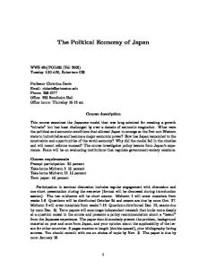
We begin this section by arguing that OPEC is a large player in the international oil markets, and that the OPEC countries benefit substantially from oil exports . We then turn to domestic fuel consumption in OPEC countries, depict the gap between domestic and international fuel prices, and show that domestic consumption in OPEC countries has changed substantially since the inception of OPEC in September 1960. In what follows, we use the amount of crude oil produced and consumed to depict the various quantity trends but use crude oil, gasoline, and diesel prices to depict the various price trends. We build on Bachmeier and Griffin (2003), who estimated an error-correction model with daily spot gasoline and crude-oil price data over the period 1985–1998 and found no evidence of asymmetry in wholesale gasoline prices, and assume that gasoline prices respond symmetrically to changes in oil prices. We also build on the technical relation between crude oil and fuels, as described below in Section 6. OPEC’s dominant position in the international oil markets is becoming more prominent over time. OPEC countries are rich in crude oil reserves, and their share of global proven reserves in 2009 amounted to 77.2%.5 Furthermore, OPEC extracted and produced roughly 45% of global crude oil production in 2008 (Fig. 1). At the same time, oil consumption in the rest of the world has been on the rise and oil extraction and production has declined. The Energy Information Administration (EIA) predicts that although non-OPEC liquids supply grew by 630,000 barrels per day (bbl/d) in 5 British

Petroleum Statistical Review of World Energy 2010 (available at http://www.bp.com/).

4

90000 OPEC Non-OPEC Former Soviet Union

80000

Thousand of barrels a day

70000

60000

50000

40000

30000

20000

10000

0

19

19

65

19

70

19

75

80

19

85

19 Year

90

19

20

95

20

00

05

20

09

Figure 1: Crude oil extraction and production – OPEC, former Soviet Union, and the rest of the world 3500

US$ (Real, 2005)

3000 2500 2000 1500 1000 500 0 1970

1975

1980

1985

1990 Year

1995

2000

2005

2010

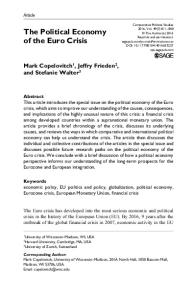
Figure 2: OPEC per capita oil export revenues 2009, in 2010 the growth rate will probably be only 420,000 bbl/d, and that rate is likely to decline to 140,000 bbl/d in 2011. World liquids demand, on the other hand, are expected to grow by 2.55 million bbl/d between 2009 and 2011.6 The increase in global demand for crude oil from 2000 to 2008 led to a significant increase in the OPEC per capita oil export revenues (Fig. 2). Nevertheless, oil revenues benefited some countries more than others: although OPEC per capita oil export revenues in 2008 amounted to 2,378 US$ (real 2005 US$), it reached 36,060 US$ in Qatar while only 446 US$ in Nigeria (Fig. OPEC country revenue). These revenue gains resulted from a rapid increase in the price of crude oil during the same period (Fig. 3). Although prices more than quadrupled, OPEC production during 1998-2010 increased by an average of only 0.6% a year and the exports grew by only 0.2% a year – suggesting a relatively inelastic supply curve.7 OPEC countries are thriving on oil export revenues but in many cases are (significantly) subsidizing domestic fuel consumption. Using data collected by Metschies et al. (2007), we computed the subsidy 6 Available 7 See

at http://www.eia.doe.gov/. EIA web site at http://www.eia.doe.gov/.

5

100 Brent West Texas Fitted line

US$

80

60

40

20

0 1975

1980

1985

1990

1995

2000

2005

2010

Year

Figure 3: World oil prices or tax equivalence levied on gasoline and diesel prices at the fuel pump. The concept of subsidization and taxation relates to a benchmark whereby fuel pricing is calculated with respect to world market prices and existing legislation. In this sense, subsidization (taxation) takes place when the actual pump price is below (above) the benchmark price. Since these benchmark prices are very difficult to calculate with precision, gasoline prices in Fig. 4 will be classified as subsidized (taxed) when they are below (above) the average US price-level, after deducting a highway tax of 10 US cents per liter on average, which is levied in the USA. The subsidy or tax equivalence levied on gasoline prices at the fuel pump are depicted in Fig. 4, which illustrates that between 2002 and 2008 nominal subsidies went up in OPEC countries, while crude oil prices increased by more than 500% (Trostle, 2008) and gasoline prices in the rest of the world surged. A similar pattern can be depicted for diesel prices. During the surge in oil prices from 2000 to 2006, and in reaction to this surge, Saudi Arabia reduced its own fuel prices by 30% – officially out of benevolence to its own population (Metschies et al., 2007).

Figure 5 depicts gasoline and diesel prices both in OPEC countries and in the rest of the world. Although from 1993 to 2000 the gap between prices in OPEC countries and the rest of the world was stable, after 2000 the gap began to grow at an increasing rate (see Fig. 5). The popular press attributed the increase in oil prices in 2000 to the OPEC production cuts agreed upon in the OPEC ministerial meetings of March 1999. Alhajji and Huettner (2000a), on the other hand, argued that low oil prices in 1998 and early 1999 led to lower upstream investment and lack of maintenance. World oil production consequently declined and many oil fields suffered from severe technical problems, which, in turn, lowered production capacity. Fuel consumption in OPEC countries has been increasing since the 1970s, in absolute terms (Fig. 6), as well as with respect to OPEC production (Fig. 7) and to world consumption (Fig. 8). During the 1990s when crude oil prices hovered between 10 and 20 US$ the ratio of consumption to production (or to world consumption) was relatively stable. From 2000 the ratio, however, did increase substantially as did crude oil prices. Oil revenues contribute significantly to disposable income in OPEC countries, which probably contributes to the increase in domestic fuel consumption in OPEC countries. In sum, OPEC has monopoly power in international oil markets, and OPEC countries use domestic

6

50 41

40

34

31 30

28

30

24

20 U. S. cents

18 10 0 -11

-10 -20

-14 -23

-21 -27

OPEC Rest of the world

-30

-32

-35

-40 1995

2000 Year

2005

Figure 4: Subsidizing petroleum fuel consumption in OPEC countries

110 100 90

Gasoline prices in OPEC countries Gasoline prices in the rest of the world Diesel prices in OPEC countries Diesel prices in the rest of the world

80

Wedge stable up to 2002, but than increased

U. S. cents

70 60 50 40 30 20 10 0 1992

1994

1996

1998

2000 Year

2002

2004

2006

0

OPEC consumption: thousand barells a day 2000 4000 6000

8000

Figure 5: The gap between fuel prices in OPEC countries and in the rest of the world

1960

1970

1980

1990

2000

year

Figure 6: OPEC consumption

7

2010

.2 OPEC consumption / OPEC production .1 .15 .05 1960

1970

1980

1990

2000

2010

year

Figure 7: OPEC consumption relative to OPEC production

0.090 0.085 0.080 0.075 0.070 0.065

Ratio

0.060 0.055 0.050 0.085

0.045 0.080

0.040 0.075

0.035 0.070

0.030 0.065

0.025 1995

0.020 1960

1965

1970

1975

1980

1985 Year

1990

2000

1995

2005

2000

2005

2010

2010

Figure 8: Oil consumption in selected OPEC countries (Algeria, Indonesia, Iran, Kuwait, Qatar, Saudi Arabia, United Arab Emirates, and Venezuela) relative to the rest of the world

8

fuel subsidies to (significantly) reduce the domestic price of fuel. However, this domestic policy is used in some OPEC countries more than in others. Building on these empirical observations, we depict in the next section our PQ-DFS model and derive the implications to international oil markets from OPEC domestic fuel consumption.

3

The production quota cum domestic fuel subsidy model

Many models have been developed to predict the OPEC pricing behavior and to model the world oil market based on the assumption that OPEC behaves like a profit-maximizing cartel. These models, however, do not fit the data well, and could not explain the gap between fuel prices in OPEC countries and in the rest of the world.8 We now develop an alternative approach, using a theoretical static trade framework, and assume politicians (not firms) run OPEC. We assume two types of countries, Home (h) and Foreign (f ) and follow the convention used in the international trade literature whereby a country f ’s variables are denoted with an asterisk (*) (Bagwell and Staiger, 2002). For tractability and without loss of generality and given that we want to explain the political economy of OPEC countries, we normalize the number of countries of type Foreign-but-not-Home to 1, and denote the country of type Foreign by F. In addition, we assume two products: fuel, denoted by subscript 1, and a numeraire good, denoted by subscript 0. These assumptions not only simplify the analysis but also enable us to focus on cheap oil policies in OPEC countries. Country h ∈ {1, ..., H} and country F are endowed, respectively, with Lh and L∗ units of the � numeraire good 0, where L = h Lh . We assume the country h produces qh units of oil, with xh � units sold domestically and mh units sold abroad (i.e., qh = xh + mh ), and we let X = h xh , � � M = h mh , and Q = h qh . Country F , on the other hand, exports the numeraire good 0. For simplicity and without loss of generality, we assume that country F does not produce fuel. In principle, the model may allow country F to produce and import oil. Then, if the oil-importing country behaves competitively, country h’s decision should simply incorporate into the calculation the net residual import demand of oil production in country F . We also assume balanced trade and balanced budget. We normalize the population in each country to 1. Following the literature on the political economy of international trade (e.g., Grossman and Helpman 1994 and 1995), preferences for a consumer in country h are captured by the following quasi-linear utility: Uh = c0h + u (c1h ) ,

(1)

8 This assumption ’as used in numerous studies on the international oil market that investigated OPEC’s pricing behavior in a static framework (Adelman 1982; Gately, 1984; Griffin 1985; Loderer, 1985; Dahl and Yucel, 1991; Gulen, 1996; Griffin and Xiong 1997; Alhajji and Huettner, 2000a and 2000b; Horn, 2004, among others). All of those studies focused on the oil market, i.e., a partial equilibrium analysis, and asked whether the international price of crude oil was the cartel (monopoly) price. Moreover, all of those papers assumed oil is extracted by profit-maximizing firms but only Griffin (1985) found statistical support for the cartel model.

9

where c0h denotes the numeraire good, c1h denotes fuel, and where ∂u/∂c1h > 0 and ∂ 2 u/∂c21h < 0. We normalize the price of the numeraire good 0 to 1. Now, let pch and mch (qh ) denote the consumer price and the marginal cost of fuel in h, respectively, and let p∗ denote the price of fuel in country F . The consumers’ total expenditure (income) in country h is Ih . With these preferences and assumptions, country h’s per capita inverse demand equals ∂u/∂c1h . The consumer in country h devotes the remainder of his total expenditure to the numeraire good, i.e., c0h = Ih − pch · c1h , thereby attaining an utility level of: Vh = Ih + CSh , where CSh = u (c1h ) − ph · c1h is the consumer surplus from fuel consumption. In equilibrium, supply equals demand, i.e., c1h = xh and c∗1 = M . We similarly define preferences in F ; namely, V ∗ = I ∗ + CS ∗ . Country h� s cost function is tch (qh ). Its derivative, mch = ∂tch /∂qh , is the marginal cost function of country h which is increasing in qh , i.e., ∂ 2 tc/∂qh2 > 0. The cost function of a finite resource can also include components like user costs. Because the dynamic aspects of oil extractions are beyond the scope of this paper, we remain agnostic with respect to the different cost components. The oil cost function of OPEC as a whole is T C (Q) = T C (X + M ). Its derivative, M C = ∂T C/∂Q, is the marginal cost curve of OPEC and is increasing in Q, i.e., ∂ 2 T C/∂Q2 > 0. We assumed that the aggregate quota, Q, is allocated efficiently among OPEC countries and not allow differences in mch – the reason is that we do not have data on differential costs of oil production among OPEC countries. Formally, we assumed that in equilibrium mch = M C for all h ∈ H. Although other quota allocation rules may be assumed (each will result in a different aggregate cost function), we elected to choose an efficient one since it allows us to compare the PQ-DFS model’s wedge with the wedge obtained under an optimal export tax model. A key assumption of the analysis is that the domestic consumer prices in OPEC countries, pch for h ∈ H, are lower than the price paid by consumers in the oil-importing countries, p∗ , and that domestic fuel prices vary among OPEC countries. This difference between the international price and the price in country h is the subsidy to consumers in country h, (i.e., subh = (p∗ − pch ) /p∗ ),

which we decomposed to two elements: a common subsidy, ϕ = (p∗ − M C) /p∗ , and a differential subsidy, sh = (M C − pch ) /p∗ ; that is, subh = (ϕ + sh ). Assuming that OPEC as a whole sets the

common subsidy, ϕ, as a wedge between international and domestic prices (and recalling that OPEC allocates the aggregate quota efficiently), M C = (1 − ϕ) · p∗ . We gain by focusing on the common subsidy because it allows us to estimate the import demand elasticity – a key parameter used in policy analysis – and to relate this elasticity to the difference between production costs and the world oil prices. Note that both the common subsidy and the differential subsidy are defined relative to the world price p∗ .

10

The differential subsidy generates a cost of Rhs = −subh · p∗ · xh , which is collected from consumers in a lump-sum fashion. Thus, the aggregate social welfare of the economy, Wh , is a function of the endowment (i.e., Lh ), the nationalized oil firm’s profits (i.e., π h = p∗ · qh − T Ch (qh )), the cost of subsidization (i.e., Rhs ), and the monetary benefits from fuel consumption (i.e., CSh ): Wh = Lh + π h +CSh + Rhs .

We similarly define welfare in country F , given that country F has only one source of income: endowment L∗ . In other words, W ∗ = L∗ + CS ∗ . In what follows, we let εh (z, y) denote the elasticity of z with respect to y in country h. We also define the supply elasticity εS ≡ ε (Q, pp ) =

pp ∂Q Q ∂pp ,

and let ε∗ =

p∗ ∂M M ∂p∗

< 0 denote the import demand

elasticity.

4

Modeling the OPEC decision process

Although, theoretically, large oil-consuming countries can exercise their monopsony power and impact the international price of crude oil (for example, by levying an import tariff or quota), the reality is that most oil-consuming countries have a limited scope for adjusting oil supply or demand in the short to medium run, particularly as oil demand becomes increasingly concentrated in the transportation sector (International Energy Agency, 2005) and the demand for oil in the light-duty vehicle sector becomes increasingly inelastic (Hughes et al., 2008).9 We thus maintain the assumption that oil-importing countries act competitively and do not exercise their market power. Our assumption follows the line of argument set forth in the literature on international trade, which assumes that countries that have market power establish policies that maximize their social welfare, taking the behavior of the rest of the world as a given. The optimal tariff literature is one branch of this literature; the literature on optimal export tax is another (see Bhagwati et al., 1998 and references therein). We focus here on two instruments used by OPEC countries to achieve domestic cheap oil policies: production quotas and fuel consumption subsidies. Because we do not empirically observe a clear sequential decision process that results in domestic cheap oil policies, we assume that the decisions are made simultaneously. We assume an OPEC wide decision and a country specific decision: OPEC 9 That said, Leiby (2007) calculates that the oil import premium is $13.60 per barrel (in 2004 dollars) with a wide 90% confidence interval ($6.70 - $23.25).

11

decision is about the production quota and the common subsidy while the country specific decision is on the deviation from the common subsidy – it is about the differential subsidy. When making a policy decision policy makers give a weight of 1 to the producer surplus but a weight of 1 + γ to the consumer surplus, both in the quota decision where we consider the entire OPEC countries and in the specific subsidy decision where we consider a specific OPEC country. Different from the the political economy literature on special interest groups, which emphasizes the production sectors and places extra weight on these sectors (Grossman and Helpman 1994 and 1995),10 we emphasize cheap oil policies and the consumers that benefit from such policies and place extra weight on the consumer surplus. When modeling the OPEC production allocation decisions, we focus on a focal equilibrium and assume politicians in countries h ∈ H collectively design the production quotas to maximize the weighted sum of the OPEC countries welfare; that is, M ax G = Q

� h

Uh + p∗ M − T C (Q) + γ OP EC · CS

(2)

H

given the differential subsidies in OPEC countries, i.e., {sh }h=1 . Whereas the OPEC countries welfare � � is h Uh +p∗ M −T C (Q), CS = h CSh denotes the sum of the consumers surplus in OPEC countries. We assume that politicians weigh consumer surplus differently than they weigh oil producers’ profits,

and let γ OP EC measure the extra weight they place on consumer surplus relative to the oil sector’s welfare. If γ OP EC > 0, then the politicians place additional weight on consumer surplus, whereas if γ OP EC < 0, then politicians care more about the oil sector’s profits. Furthermore, when politicians care only about the oil companies’ profits, then γ OP EC = −1, and we revert to the classic cartel-offirms model. The estimated value of γ OP EC can, therefore, be used to assess the plausibility of the alternative models. Similarly, we assume that politicians, when setting the differential country-specific fuel subsidies, weigh consumer surplus differently than they weigh oil producers’ profits and revenue. Formally, let γ h measure the extra weight politicians place on consumer surplus relative to the oil sector’s welfare. When modeling the domestic decisions in OPEC countries we assume that politicians in country h maximize M ax Gh = Wh + γ h · CSh , sh

(3)

by choosing non-cooperatively the differential country-specific fuel subsidy sh – that is, they choose H

sh given the allocation of production quotas, {qh }h=1 , and thus the common subsidy, τ , and given the differential country-specific subsidies set by other OPEC countries, {sj }j�=h . Although OPEC countries cooperate when deciding on the allocation of production quotas, domestic policy is subject to domestic scrutiny and may be viewed as a sign of sovereignty. 10 See

also Gawande and Krishna (2003), and references therein.

12

At the equilibrium: (2) the allocation of the production quotas is optimal given the level of the domestic fuel subsidies set by OPEC countries; and (3) the subsidy set by an OPEC country is optimal, given the allocation of quotas among OPEC countries and given the subsidies set by other OPEC countries.

5

The equilibrium outcome and its implications

We now derive and characterize the equilibrium outcome, and discuss its implications. We begin with the allocation of production quotas among OPEC countries (Section 5.1), and continue with the optimal political economic fuel subsidies in OPEC countries (Section 5.2).

5.1

OPEC production quotas

OPEC countries respond to market fundamentals and forecast developments by co-ordinating their production quotas while taking domestic subsidies as given. Saudi Arabia, for example, maintained its domestic prices, while coordinating production quotas among OPEC countries: “One industry source estimated Saudi Arabia had reduced exports, as opposed to production, by around 900,000 barrels per day compared with a peak in August [2008].”11 Proposition 1 At the optimal allocation of production quotas ϕ=

�

1−

where the common subsidy ϕ =

�

c1h h M

· (εh (c1h , pch ) · sh + γ OP EC · (1 − sh )) � � 1h � −ε∗ − γ OP EC h cM

p∗ −M C . p∗

�

(4)

Furthermore, if both the numerator and the denominator of

Eq. (4) are positive (i.e., the extra weight placed on domestic fuel consumption, γ OP EC , is sufficiently close to zero), then the following results in a larger common subsidy, ϕ:

• a decrease in the absolute value of the price elasticity of the import demand curve, ε∗ ; • an increase in the absolute value of the price elasticity of the domestic fuel demand, εh (c1h , pch ); • an increase in the differential subsidy, sh ; and, • given that the benefits from subsidizing domestic fuel prices in OPEC countries are sufficiently

sh large, i.e., γ OP EC < 1−s · εh (c1h , pch ), an increase in the ratio of domestic fuel consumption h � c1h to exports, i.e., h M , will result in a larger common subsidy, ϕ.

11 Available

at CNBC.com, November 4, 2008.

13

Proof: The condition is derived by taking the first order condition of (2), while using the market clearing conditions whereby world demand equals world supply and holding sh for all h constant.

Q.E.D.

Equation (4) states that at the optimal solution the ratio (p∗ − M C) /p∗ equals �

1−

�

c1h h M

� · (εh (c1h , pch ) · sh + γ OP EC · (1 − sh )) � � � 1h . −ε∗ − γ OP EC h cM

Alternatively, this ratio equals the common subsidy, ϕ. The ratio is one over the absolute value of the import demand elasticity, −ε∗ , while correcting for the benefits and costs of subsidization. Clearly, monopoly power in international markets affects the optimal pricing rule, where a lower import demand elasticity (in absolute value) results in a larger common subsidy. While oil demand is becoming increasingly concentrated in the transportation sector (World Energy Outlook, 2005) and the demand for oil in the light-duty vehicle sector is becoming increasingly inelastic (Hughes et al., 2008), the wedge between prices in OPEC and non-OPEC countries is increasing. However, introducing domestic fuel subsidies results in two additional forces that affect this optimal pricing rule: the benefits to consumers in OPEC countries from lower fuel prices, and the cost to consumers from subsidizing fuel consumption. Then, if the extra weight placed on fuel consumption, γ OP EC , is sufficiently small, a larger (relative) amount of fuel consumed in OPEC countries results in a higher common subsidy, i.e.,

p∗ −M C p∗

and thus ϕ are larger. The stylized facts presented in Section

2 fits the theory’s predictions, as long as the weight OPEC places on domestic fuel consumption is sufficiently small in absolute value. Indeed, we observe a relative increase in domestic consumption in OPEC countries (Fig. 6) that is coupled with an increase in qh /mh (Fig. 7) and an increase in world oil prices (Fig. 3), both of which the theory predicts should increase ϕ. As documented in Fig. 4, subsidies in OPEC countries (i.e., subh for h ∈ {1, ..., H}) have indeed increased during the latest surge in oil prices, which began in 2000, and the spike in OPEC oil consumption that accompanied it. The ambiguous effect of the extra weight placed on consumers, γ OP EC , on the common subsidy, ϕ, is because this extra weight multiplies the consumer surplus but not the cost of subsidization (or the profits from the nationalized oil companies). We believe such a representation makes sense, because consumers understand the direct implications from lower fuel prices but the implications from government transfers and government investment in public goods are less transparent to them. Moreover, because the only difference between the cost of subsidization and profits from the nationalized oil companies is that one decreases while the other increases the government revenues, it is reasonable to assume that policy makers place the same weight on the oil sector and on the cost of subsidization when making policy decisions.

14

Corollary 1 Given no differential country-specific fuel subsidies in OPEC countries (sh = 0 for all h ∈ H) and no extra weight placed on fuel consumers (γ OP EC = 0), setting an aggregate production quota results in the same outcome as if OPEC sets an optimal export tax. Alternatively, if fuel consumption in OPEC countries equals zero (c1h = 0 for all h ∈ H), setting an aggregate production quota results in the same outcome as if OPEC sets an optimal export tax.

Proof: Follows directly from Proposition 1, given that sh = 0 for all h ∈ H and γ OP EC = 0. Alternatively, the results follow given that c1h = 0 for all h ∈ H. Q.E.D.

When OPEC decisions are limited to setting the production quotas that maximize aggregate welfare (no differential subsidies), then the common subsidy defined above equals the optimal export tax, i.e., ϕ = − ε1∗ .12 The only difference is in the interpretation: When the optimal export tax is derived, the reference price is the domestic price and the international price is the domestic price plus the export tax. When setting a production quota, on the other hand, the reference price is the international price and the domestic price is the international minus the common subsidy.

5.2

The differential subsidies in OPEC countries

We now solve for the optimal fuel subsidy in country h ∈ H under two alternative scenarios: the decoupled scenario and the integrated scenario. We begin by deriving the fuel subsidy where domestic fuel policies in OPEC countries do not affect world fuel demanded, which is what the literature on OPEC usually assumes, and we denote this scenario the decoupled scenario. Next, we derive the conditions under which such a scenario is plausible. But because, empirically, these conditions are not satisfied (Section 2), we expand our decoupled scenario to one in which cheap oil policies in OPEC countries do affect world prices, coin it the integrated scenario, and characterize the equilibrium under this alternative scenario. The integrated scenario is the scenario we used to construct the empirical model depicted in Section 7.

The decoupled scenario and its implications

When characterizing the optimal fuel subsidy

under the decoupled scenario, we assume production quotas are fixed and are not affected by the domestic subsidies in OPEC countries. The majority of literature on OPEC makes this assumption, and decouples domestic fuel and oil policies in OPEC countries from the production allocation decisions in those countries. 12 Similar results are obtained in Grossman and Helpman (1995), when the government sets trade policy that maximizes aggregate welfare and does not place extra weight on the special interest groups.

15

Proposition 2 Assume production quotas, qh , and international prices, p∗ , are given. The domestic fuel subsidy in country h then equals

subh =

− εh (pch1 ,c1h )

1 γh

−

1 εh (pch ,c1h )

.

Furthermore,

• if γ h → 0 then subh → 0 and sh → −ϕ, but if γ h → ∞ then subh → 1 and thus sh → 1 − ϕ and pch → 0. • The differential subsidy, sh , – increases monotonically with γ h , – and decreases with |εh (c1h , pch )|. Proof: To derive the optimal fuel subsidy in country h under the decoupled scenario, we assume that production is fixed (i.e., the common subsidy is fixed) and thus focus only on the component of country h’s objective function, i.e., Eq. (3), that is directly related to domestic consumption. Taking the first-order derivative with respect to sh , we obtain subh =

We know that

∂pch ∂subh

(1 + γ h ) p∗ − pch pch − . ∂pch ∗ γh p εh (pch , c1h ) ∂sub h

= −p∗ , and thus subh = ϕ + sh =

− εh (c1h1 ,pch )

1 γh

−

1 εh (c1h ,pch )

=

γh − εh (pch ,c1h )

1+

γh −εh (pch ,c1h )

(recall that pch = (1 − subh ) p∗ ). Q.E.D.

The assumptions made regarding the decoupled scenario result in the following optimal political economic fuel subsidy for country h ∈ H: subh =

− εh (c1h1 ,pch )

1 γh

−

1 εh (c1h ,pch )

=

γh − εh (pch ,c1h )

1+

γh −εh (pch ,c1h )

.

(5)

Equation (5) suggests a positive correlation between the weight placed on consumer surplus and the subsidy chosen (i.e., γ h ↑⇒ subh ↑): the greater the weight given to consumers, the higher is the optimal fuel subsidy. Furthermore, if politicians care only about domestic fuel consumers, then

16

subh = 1 (i.e., γ h→∞ lim γ1 = 0). If, however, politicians care about domestic welfare and do not h

favor one group over the other, then γ h = 0 as well as subh = 0. A more inelastic demand for fuel in OPEC countries (i.e., |εh (c1h , pch )| is smaller) results in a higher domestic fuel subsidy at equilibrium. The decoupled scenario assumes that the differential subsidies in oil-exporting countries do not affect world prices; in other words,

dp∗ dsh

= 0 for all h ∈ H. We now derive conditions under which such

an assumption would be consistent with our conceptual framework. Proposition 3 If

• domestic demand in country h is inelastic, i.e., εh (c1h , pch ) → 0, or • consumption in country h is very small, i.e., c1h → 0, or • demand in country F is very elastic, i.e., ε∗ → ∞, then

dp∗ dsh

→ 0.

Proof: The proof is relegated to Appendix A.

If domestic demand in OPEC countries is very inelastic, i.e. large changes in prices result in very small changes in quantities or the marginal cost curve is basically flat, then it is reasonable to assume that domestic fuel subsidies in OPEC countries do not affect world fuel prices. If, also, fuel consumption in OPEC countries is very low, then the link between the domestic fuel subsidy and OPEC pricing behavior is of little importance. However, as argued in the Introduction and in Section 2, and as our empirical estimates validate, these conditions do not capture the real world in which OPEC countries set both production quotas and domestic fuel subsidies.

The integrated scenario. We now investigate this link between domestic fuel subsidies in OPEC countries and OPEC production quotas, and show how domestic policy in OPEC countries spills over to world fuel markets. To this end, we extend our conceptual framework and note that given the allocation of quotas,

dp∗ dsh

> 0 (see Appendix B).

Proposition 4 The fuel subsidy in country h is set such that

subh =

γh −εh (c1h ,pch ) γh −εh (c1h ,pch )

1 −εh (mh ,p∗ )

1+

Proof: The proof is relegated to Appendix B.

17

+

(6)

Proposition 4 shows that, unlike the decoupled scenario discussed above, the allocation of production quotas affects the optimal level of the fuel subsidy. Proposition 1 shows, however, that domestic policy in OPEC countries affects the optimal production allocation rule. Together Propositions 1 and 4, therefore, suggest that cheap oil policies in OPEC countries affect the OPEC trade policy, and that the OPEC trade policy affects the choice of domestic policies in OPEC countries. The optimal subsidy is determined not only by the domestic demand elasticity, εh (c1h , pch ), and the extra weight placed on the consumers surplus, γ h , but also by the import response elasticity, εh (mh , p∗ ). That is, although the optimal subsidy under the decoupled scenario equals

1 it equals

γh −εh (c1h ,pch ) h + −εh (cγ1h ,pch )

γh −εh (c1h ,pch ) γh −εh (c1h ,pch )

1 −εh (mh ,p∗ )

1+

,

+

under the integrated scenario. Note that if εh (mh , p∗ ) < 0 then, all else being equal, the differential subsidy is larger under the integrated scenario. Furthermore, if the extra weight placed on domestic fuel consumption, γ OP EC , is sufficiently close to zero, then the wedge between the prices in OPEC countries and the international price are larger under the integrated scenario. Higher domestic fuel subsidies result in more domestic consumption. The increase in domestic consumption comes at the expense of export, such that c1h increases and mh decreases. Building on the integrated scenario developed above, we derive an empirical model which we then estimate. We estimate the demand functions, and then use these estimates together with the estimated subsidy equation parameters to compute the extra weight placed on consumer surplus in OPEC countries. Note that demand estimates are derived independent of our conceptual model, and the equilibrium behavior is only introduced through the subsidy equation. Furthermore, the quota allocation rule assumed above does not affect the empirical results and the extra weight placed on consumer surplus in OPEC countries is estimated independent of the allocation rule. However, using data from the EIA, we derive similar results for OPEC as an organization. We begin the empirical analysis by describing the data and its limitations (Section 6). Then, we incorporate the data constraints into our empirical model (Section 7). The empirical findings are reported in Section 8, in which we also assess the validity of the alternative models discussed in the literature.

18

6

The data

We estimate the empirical model using data on annual quantities of crude oil taken from the British Petroleum Statistical Review13 . Prices used are fuel prices at the pump (in constant 2006 US$) taken from Metschies et al. (2007) and from the GTZ International Fuel Prices, 6th Edition.14 Although we aim to explain differences in fuel prices among oil-exporting and oil-importing countries, we have global data only on oil production and consumption, but not on gasoline and diesel consumption. However, using data from the U. S. Energy Information Administration website (EIA)15 we can show that although crude oil is used to produce several products ranging from gasoline and diesel to asphalt and oil lubricants, 65% to 67% of every barrel of crude oil in the United States from 1993 to 2008 was allocated to the production of gasoline and diesel. These two products, characterized by relatively high profit margins compared with other crude products, are the main source of income of downstream refineries.16 This creates strong incentives for refineries to maximize the amount of gasoline and diesel produced from crude, an amount that is constrained by technology.17 We, therefore, assume a fixedproportion relationship between crude oil and fossil fuel consumed, i.e., the quantities of fossil fuel consumed can be derived from the quantities of crude oil and the optimal quantity of fuel consumed determines the quantity of crude oil demanded. Specifically, a barrel of crude oil yields 19.5 gallons of gasoline and 8.5 gallons of diesel, on average. This represents 67% of a barrel of crude oil, with the remaining volume used to produce kerosene-type jet fuel, liquefied refinery gases, still gas, coke, asphalt and road oil, and petrochemical feedstock.18 We use this ratio to convert barrels of crude oil to fuel consumed, and to compute the weighted average price of fuel at the pump, i.e., 19.5/28 × gasoline price plus 8.5/28 × diesel price.19 We focus on aggregate fuel consumption (gasoline and diesel) because we believe that both types of fuel affect demand for crude oil, and thus the composite model better captures the interactions between crude oil and the downstream fuel market. To estimate our empirical model we had to control for other effects, while correcting the estimation procedures for endogeneity and mis-specification problems. Thus, when estimating domestic demand in the OPEC countries we expanded our price and quantity data set to include OPEC-country-level data: purchasing power parity, energy consumption per capita, and car ownership. When estimating the import demand and cost equations, we included data on world GDP per capita, GDP per capita for developed countries and for emerging countries, GDP growth rates, OPEC capacity, OPEC production 13 Available

at http://www.bp.com/ data presented in these two sources is for 1993, 1995, 1998, 2000, 2002, 2004, 2006, and 2008. 15 See http://tonto.eia.doe.gov/dnav/pet/pet pnp pct dc nus pct m.htm 16 According to Tom Campbell, a commercial manager at BP, this ratio is used to approximate the highly valuable fuel content of crude oil. 17 The evolution of the petroleum refinery industry is one in which the main objective of technological innovations, dating back to the 1940s, is to maximize the amount of gasoline and diesel produced from a barrel of crude oil. See, for example, Leffler (1985) and Jones and Pujado (2008). 18 http://www.txoga.org/articles/308/1/WHAT-A-BARREL-OF-CRUDE-OIL-MAKES. 19 Although we could adjust these weights using global data on refined fuels, with the objective of capturing changes in the composition of a barrel of crude oil over time (available from Oil & Gas), we elected to maintain the weights presented above, because the year-specific weights are computed based on global refining capacity (not only OPEC oil) and introducing these year-specific weights does not change the results much. 14 The

19

quotas, and OPEC reference basket price. The different variables and the sources used are summarized in Appendix C.

7

The empirical model

To estimate cheap oil policies in OPEC countries, we assume constant elasticity of demand and cost functions.20 Furthermore, to transition from the conceptual model discussed above to the empirical model estimated below, error terms should be introduced and their distribution specified. Since the theory is silent about the error terms and their structure, we assume additive error terms. Specifically, we assume the following for the domestic demand for fuel in country h: ln (pch ) = φ0 − φ1 · ln (c1h ) + Γc Zch + ς Ch .

(7)

where vector Zch denotes the log of control variables such as GDP per capita (which controls for income) and purchasing power parity (which controls for real exchange rate fluctuations), and ς Ch denotes the error term. We expect that the estimated parameters will be positive, i.e., 0 < φ0 , φ1 , suggesting that prices decline with the quantity of fuel consumed and that price elasticity in country h is −1/φ1 < 0. The official documentation on the OPEC website suggests OPEC Reference Basket prices guide OPEC’s production decision, and that OPEC’s production ceiling decisions (i.e., quota allocation) are guided by this basket price. We therefore assume that the world price, i.e., p∗ , is the OPEC Reference Basket price. The OPEC import demand curve is given by: ln (M ) = β 0 − β 1 ln (p∗ ) + ΓM ZM + ς M

,

(8)

where vector ZM denotes the log of the control variables, which includes world GDP per capita as well as GDP per capita of developed and emerging countries. Let ς M denote the error term. We expect that 0 < β 0 , β 1 . Finally, if we assume ε (mh , p∗ ) is fixed (as implied by a constant elasticity structure, while assuming OPEC countries adhere to the production quota set at the OPEC ministerial meetings and that the production quota share of an OPEC country is constant throughout the investigated period – to this end, the OPEC countries production shares were very stable throughout the investigated period with quotas for most countries changing by less than 1%), then the differential subsidy equation depicted in Proposition 4 can be estimated as follows: p∗ = κh · pch + ς sh . 20 Numerous

(9)

papers set forth these assumptions, including Chakravorty et al. (1997) and Kauffmann et al. (2008).

20

Let ς sh denote the error term. Our assumptions regarding ε (mh , p∗ ) result in the parameters κh , which equals

�

� γh 1 − εh (c1h ,pch ) �. κh = � 1 1 + εh (mh ,p∗ )

Equation (9) suggests that, if ∂mh /∂M = mh /M 21 then γh =

�

�

1 1− 1+ ∗ ε

�

· κh

�

· εh (c1h , pch ) .

Although the theory predicts differences among OPEC countries and preliminary analysis indeed supports this heterogeneity, we do not report here estimates of the country-specific parameters since the number of observations per country is too small (less than 10), and so we confine the discussion to a common extra weight placed on consumer surplus in OPEC countries. In other words, we estimate p∗ = κ · pch + ς s

(10)

using instrumental variable techniques. In sum, we estimate a parsimonious model that draws from our conceptual framework, i.e., ln (pch )

=

b0 + b1 ln (c1h ) + b2 · Zch + ς Ch

(11a)

ln (p∗ )

=

d0 + d1 ln (M ) + dM ZM + ς M .

(11b)

And then use these estimates, together with Eq. (10), to compute the extra weight the politicians in OPEC countries place on consumer surplus, i.e., γ h = γ H for h ∈ H. The estimated parameters are used to calculate the parameters of the structural model as follows:

21 ε

h

(mh , p∗ ) =

∂mh p∗ ∂p∗ mh

=

φ0

=

b0 ,

φ1

=

β1

=

β0

=

γH

=

−b1 , 1 − , d1 d0 − and d � 1 � κ1 1 1− (1 + d1 ) . κ0 b1

∂mh ∂M p∗ M . ∂M ∂p∗ M mh

Thus, if ∂mh /∂M = mh /M then εh (mh , p∗ ) = ε∗ .

21

This notation suggests that εh (c1h , pch )

=

ε∗

=

ε (Q, M C)

=

1 1 = , ϕ1 b1 1 −β 1 = , and d1 1 1 = . ρ1 a1 −

Using the above estimates, together with cost estimates supplied by the EIA (2007), while building on Equation (4), we can also compute the extra weight OPEC gives fuel consumers in OPEC countries when allocating quotas: γ OP EC =

1−

�

c1h h M · εh (c1h , pch ) · sh � c1h h M (1 − subh )

+ ϕ · ε∗

(14)

The marginal cost estimates are used to compute the common subsidy, ϕ = (p∗ − M C) /p∗ , and the

differential subsidy, sh = (M C − pch ) /p∗ , and thus the value of the domestic fuel subsidy in OPEC countries, subh = ϕ+sh . These estimates, together with the estimated parameters ε∗ and εh (c1h , pch ) and the data on consumption and exports, are used to estimate the value of γ OP EC using non-linear estimating techniques. Note that if c1h = 0 for all h ∈ H and γ OP EC = 0, then ϕ = −1/ε∗ . The common subsidy equals one over the absolute value of the import demand elasticity – the common subsidy equals the optimal export tax.

8

The empirical analysis

We now estimate the empirical model, which includes Eqs. (10) and (11), and report the results. The fundamental assumption for consistency of least square estimators is that the error terms are unrelated to the regressors. We cannot, however, make this argument here. Our equations are derived from theory and each equation purports to describe a particular aspect of the economy. The model is one in which price and quantity are determined jointly, and where the volume of trade may be endogenously determined together with trade barriers (Trefler, 1993). The endogeneity problem suggests that the error term embodies factors not explained by the regressors, and that some of the unobserved factors that are captured by the error term may be correlated with the regressors. One solution to this problem, which can correct for this endogeneity bias, would be to include, as regressors, controls for the unobserved factors, i.e., the control variable approach. We apply this approach when estimating our domestic demand equation. For example, because higher GDP per capita may be correlated with a higher propensity to spend on a given good, we include these variables in our empirical equation. We do not, however, control for all such factors,

22

as the empirical analysis presented below suggests, simply because we could not find all the regressor controls we were looking for. Thus, we resort to the instrumental variable approach, which introduces instrumental variables that are associated with the regressors but not with the error term. To this end, we use economic theory to free up variables from the estimated equation that are correlated with the included endogenous variables. We estimate this over-identified set of equations using two-stage least square (2SLS) techniques, an asymptotically efficient estimator if indeed the error terms are independent and homoskedastic. Data points on prices and quantities taken over time may have an internal structure that should be accounted for. We, therefore, test the data for non-stationarity and de-trend it when needed. We also convert current prices and GDP per capita to constant 2005 US$. Our set of equations relies on two different data sets. Whereas Eq. (11b) is estimated using aggregate data at the OPEC level, Eqs. (10) and (11a) rely on country-level data. We thus apply estimation techniques using limited information estimation methods, which neglect information contained in other equations.22 Focusing on limited information estimation techniques will enable us to compare our estimates to those obtained using limited information maximum likelihood (LIML) estimators, which are asymptotically equivalent to 2SLS but have different finite-sample properties – thus checking the robustness of our estimates. The difference between LIML and 2SLS in finite samples stems from the difference in the weights placed on instruments. These differences result in smaller biases under LIML, especially when the instruments are weak (Cameron and Trivedi, 2010). Our baseline model is the model derived using 2SLS techniques, whose parameters are depicted in Tables 4 and 5. The first equation estimated is the domestic demand for fuel in OPEC countries (i.e., Eq. 10). Here, we add control variables that capture the income effect on demand for fuel, namely, GDP per capita in country h (denoted GDP per capitah ), and the value of money in OPEC countries measured by the quantity and quality of products and services consumers can buy, namely, the purchasing power of country h (denoted P P Ph ). Furthermore, since the model is one in which prices and quantities are determined jointly, we use supply shifters such as production variables to identify the demand equation’s regressors. We also introduce two additional variables that capture two sources of demand for fuel: population (denoted populationh ) and per capita energy consumption (denoted energy perCapitah ). In addition to the above control variables, supply variables were used as instruments (production and quotas). The specification of the baseline scenario, which was estimated using 2SLS techniques, is pch = exp−27.34 ·c−1.72 · GDP per capita1.18 · P P Ph−0.26 · population0.57 · energy perCapita0.20 h h h . 1h 22 Moreover, although the system methods [e.g., three-stage least square (3SLS)] are asymptotically better, the advantage is not clear when the analysis is confined to a finite sample. The finite sample variation of the estimated covariance matrix is transmitted throughout the system, and may result in the 3SLS having a larger finite sample variance than that of the 2SLS or the LIML. In addition, the limited information methods not only limit the variation of the parameters in a finite sample, but also confine any structural problem in a particular equation to the equation in which it appears.

23

This analysis suggests that the average elasticity of domestic demand for petroleum fuels used for transportation, electricity, and heat in OPEC countries is εh (c1h , pch ) =

1 = −0.58 −1.72

whereas the income elasticity is 0.68 = 1.18/1.72. These elasticities are consistent with estimations reported in the literature and result in both price and income elasticity well below 1, in absolute value. To this end, Goodwin (1992) computes in his review a simple mean value of 120 elasticity of gasoline consumption with respect to fuel prices, which equals -0.48. We must, however, take care when making this comparison with the literature. First, our focus is on OPEC countries, a set of oil-exporting countries that do not appear in most, if not all, studies. In these countries, large parts of the population receive free electricity that is partly produced from fuel. Although the Qatar government has limited the provision of free electricity to Qatari-citizen households since 1999, with payment required for consumption above a set threshold, electricity is still heavily subsidized. Second, we use biennial data, suggesting that we are estimating the medium-run elasticities. We now report on import demand parameters. We begin by testing the data for unit-root using the augmented Dickey–Fuller test (Dickey and Fuller, 1979) that a variable follows a unit-root process. The null hypothesis is that the variable contains a unit root, and the alternative is that the variable was generated by a stationary process. We cannot reject the null hypothesis at a 1% significant level, for either prices or exports. We then produced the Trace statistic (Johansen, 1995) to determine the number of cointegrating equations in a vector error-correction model. We cannot reject the null hypothesis at a 5% significant level that there are one or fewer cointegrating equations. Therefore, when estimating Eq. (11b), we took first differences of the world prices and quantities consumed. The ordinary least squares (OLS) estimators are consistent when the regressors are exogenous, and optimal in the class of linear unbiased estimators when the errors are homoscedastic and serially uncorrelated. Therefore, when testing to determine whether endogenous regressors in the model are in fact exogenous, and being unable to reject the null hypothesis that the regressors are exogenous at a 1% significant level, we elected to report the OLS estimators in the baseline scenario (see Section 8.1, in which the various tests were performed and reported, as well as the regressors estimated, using instrumental variable techniques). That is, we estimated the following equation � � ln (p∗t ) − ln p∗t−1

=

−0.72 · (ln (Mt ) − ln (Mt−1 )) +2.07 · (ln (W incomet ) − ln (W incomet−1 )) + 0.0000676 · t × dummyyear>98

where world GDP per capita at time t is denoted W incomet . Using the Chow test, we identified a structural break in 1998. We, thus, introduced a dummy variable that equals 1 for the years

24

1999 to 2008, denoted dummyyear>98 . The import demand elasticity observed by OPEC equals −1.39 = −1/0.72.23 Then, since in 2006 OPEC produces about 45 percent of world oil consumption, the empirical model suggests a world demand elasticity of about −0.62, which is within the range of medium- to long-run price elasticities reported in the literature (Cooper, 2003; Leiby, 2007). Furthermore, Sterner (1990) examines the pricing and consumption of gasoline in OECD countries reported in the literature and concludes that long-run price elasticity falls in the interval -0.65 to -1.0 and for income between 1.0 and 1.3. On the other hand, Ramanathan (1999) found that the long-run income elasticity of gasoline in India is quite high, at 2.682. OPEC countries pursue cheap domestic fuel prices. Using Eq. (10), we compute an estimate for the average γ in OPEC countries. We begin by testing the data for unit-root using the augmented Dickey–Fuller test. We cannot reject the null hypothesis at a 1% significant level, for either prices (note that while the domestic demand is linear in logs, Eq. (10) is linear in the prices). We also cannot reject the null hypothesis at a 10% significant level that there are one or fewer cointegrating equations. Therefore, when estimating Eq. (10), we took first differences of the world prices and the domestic prices in OPEC countries and employed instrumental variable techniques that have been extended to fixed effect models. We elected to use fixed effects techniques when estimating Eq. (10) because we could not reject the hypothesis that such effects exist. That is, we assume all OPEC countries assign the same extra weight γ to consumer surplus, i.e., γ h = γ H for all h ∈ H. This equation was estimated using bi-yearly data on fuel prices in OPEC countries, from 1993 to 2008, while excluding Angola, Ecuador, Iraq, Libya, and Nigeria due to missing data. Using the estimated parameters, we compute the average γ in OPEC countries: γ H = 0.32 In other words, the ruling party in an OPEC country places about 32% more weight on consumer welfare from fuel consumption. This stands in contrast to work that builds on Grossman and Helpman (1994) and is applied to the United States, suggesting that when setting trade policy, governments place only a few percentage points on the interest groups’ welfare compared with aggregate welfare (Goldberg and Maggi, 1999; Gawande and Bandyopadhyay, 2000). Branstetter and Feenstra (1999), on the other hand, who examined trade and foreign direct investment (FDI) in China using provincelevel data on trade and FDI flows to estimate parameters of the government’s objective function, found that the government places on consumer welfare only half the weight that it places on the welfare of state-owned enterprises. Although our sample size does not permit us to estimate the weights, γ h , which vary among OPEC countries, we have documented significant differences across countries – differences that are systematic 23 When estimating the import demand function using the West Texas intermediate, as opposed to the OPEC basket price, the elasticity equaled −2.08.

25

across regions. To illustrate these differences we focus on 2006 and present country-specific subsidies for both gasoline and diesel (Table 3). The table also includes proven reserves and the ratio of exports to production for that year. Our theory predicts that a lower export to production ratio will result in a higher domestic subsidy. Although we can not control for all factors, the correlations between the domestic fuel subsidies for gasoline and diesel and the ratio of exports to production in Indonesia, Iran, Venezuela, Saudi Arabia, UAE, Algeria, Kuwait, and Qatar are −0.63 and −0.36, respectively (no data is available for other OPEC countries for 2006) . We also computed the correlation coefficient between proven reserves and the domestic fuel subsidies in OPEC countries. Here, we get −0.52 and −0.43 for gasoline and diesel, respectively, where now the list of countries included Angola, Libya, and Nigeria, in addition to the eight countries mentioned above. This seems to suggest that OPEC countries view crude oil reserves as an endowment, and use this endowment to transfer money to (fuel) consumers. Then, if larger reserves suggest lower user costs (i.e., lower cost from extracting oil today as opposed to the future), then, all else being equal, we should get more subsidization in those countries. Country

Indonesia Angola Algeria Qatar Nigeria Libya Venezuela UAE Kuwait Iran SaudiArabia

Gasoline price (World price equals 53 cents per litter) 108% 94% 60% 36% 96% 25% 6% 70% 42% 17% 30%

Diesel price (World price equals 59 cents per litter) 75% 61% 32% 32% 112% 22% 3% 90% 36% 5% 12%

Proven reserves (Thousand million barrels) 4.4 9 12.3 27.4 36.2 41.5 87.3 97.8 101.5 138.4 264.3

exports/production

-0.15 . 0.87 0.93 . . 0.78 0.86 0.90 0.60 0.83

Table 1: Difference among OPEC countries Parameter γ H tells us how much extra weight politicians, who control the domestic oil industry and set domestic fuel prices, place on consumer surplus from fuel consumption compared with aggregate welfare. We now use this parameter, and the standard deviation associated with it, to evaluate the plausibility of other competing theories. We begin with the textbook cartel theory, namely, the cartel of firms. If OPEC allocated production quotas as if it were a cartel of firms, then γ H = −1, and we will not reject the hypothesis that γ H = −1. However, our estimated subsidy equation, taking the import demand elasticity and the domestic demand elasticity as given, results in a 95% confidence interval for the γ H parameter of [−0.65, 1.31], which is well above −1. To conclude, the baseline model suggests that OPEC countries do not maximize aggregate domestic welfare but that they place additional weight on domestic fuel consumption, much like countries that set cheap food policies and subsidize domestic food consumption to achieve political stability and cheap labor.

26

Demand for cheap fuel in OPEC countries is also affecting OPEC production decisions. Using Eq. (14) and the cost estimates provided by the EIA (2007), we computed γ OP EC . The EIA (2007) supplies the lifting costs (also called production costs), which are the out-of-pocket costs to operate and maintain existing production wells and related equipment and facilities per barrel of oil equivalent of oil and natural gas produced by those facilities after the hydrocarbons have been found, acquired, and developed for production. The highest lifting costs reported for an OPEC country were in Africa and equaled 5.66 US$. The calculated γ OP EC depends on the cost component used. There are different degrees of support among studies to the extent to which the Hotelling Valuation Principle affects oil supply (e.g., Miller and Upton, 1985; Adelman and Watkins, 1995; Lin, 2007; Hamilton, 2009). Therefore, because in principle the cost of extraction and production of oil and fuel should incorporate these Hotelling rents, we choose three plausible costs for the analysis: (i) 5.66 US$; (ii) 5.66 × 1.125 = 6.368 US$; and (iii) 5.66 × 1.25 = 7.075 US$. These costs generate three different values for γ OP EC : Marginal cost

γ OP EC

5.660

0.10

6.368

−0.24

7.075

−0.63

That is, if indeed decisions are guided only by current costs, then the OPEC optimal pricing rule can be approximated by a pricing rule derived as though OPEC maximizes aggregate welfare when setting production quotas. OPEC countries exploit their monopoly power in international oil markets and the analysis suggests that implicitly the optimal export tax explains well the average wedge observed in OPEC countries, and that on average OPEC maximizes OPEC countries social welfare when making production decisions.

8.1

Robustness of results

We now report on the post estimation analysis used to evaluate the robustness of our results. We begin with the cost function, continue with the domestic demand for fuel and the import demand function, and conclude with the subsidy equation.

The domestic demand for fuel

Except for the amount of electricity per capita, all baseline

parameters were significant at a 5% level, and the 2SLS resulted in R2 = 0.3070 (Table 4). As for the post-estimation analysis, we began by testing for endogeneity using two alternative tests: the Durbin test (Durbin, 1954) and the Wu-Haisman test (Wu, 1974, and Hausman, 1978). Endogeneity tests determine whether endogenous regressors in the model are in fact exogenous, where the null

27

hypothesis is that the variables are exogenous. We rejected the null hypothesis under both tests at a 1% significance level and report the Durbin and Wu-Hausman statistics in Table 2 Test Durbin (score) Wu-Hausman

Statistic 9.98 11.47

P-value p=0.0016 p=0.0025

Table 2: Durbin and Wu-Hausman tests However, even if the instrumental variables are consistent, they may be weak in which case the asymptotic theory provides a poor guide to actual finite-sample distribution (Davidson and MacKinnon, 2004). Here, we use Stock and Yogo’s (2005) methodology and apply two complementary test approaches. The first approach addresses the concern that the estimation bias of the instrumental variable estimators from the use of weak instruments can be large, sometimes even exceeding the bias of the OLS. The test statistic for this approach is the F-statistic for joint significance of instruments in the first-stage regression, which was found to be 10.6383. This statistic is greater than the widely used rule of thumb of 10.00 (Staiger and Stock, 1997). The second approach addresses the concern that weak instruments can lead to size distortions of Wald tests performed on the parameters of finite samples. This latter approach uses Shea’s partial R2 , which is 0.48 and went on to compute the pairwise correlation coefficients, noting that the gross correlations of the instruments with the endogenous regressor are greater than 0.8. We thus concluded that our instruments are not weak. To evaluate the sensitivity of the estimated parameters, we compared our estimates to those obtained using alternative techniques, namely, OLS and LIML. Although under the OLS estimating techniques, we ended up a different domestic demand elasticity (Table 4), using LIML techniques to estimate the demand function resulted in estimates similar to those obtained under 2SLS. Returning to the 2SLS techniques, we also tried other specifications, including dropping the control variables and replacing them with other variables, as well as introducing different instruments. The outcome under these alternative specifications resulted in a much lower adjusted R2 . Although for each country the number of observations over time is relative small, the data used to estimate the domestic demand for fuel in OPEC countries potentially may include non-stationary variables. Though we believe that the time-series properties of the biennially data from 1993 to 2008 for the different OPEC countries is of secondary importance, we did compute and regress first differences. Even though the parameters did not come significant, the size of the demand elasticity is very similar to the one we estimated in our baseline model – the differences are in the second decimal point.

The import demand elasticity.

Looking at first differences and dropping the constant term

resulted in independent variables that are not correlated with the error term, i.e., the independent

28

variables measured as first differences are exogenous. Using 2SLS or LIML, the null hypothesis that the variables are exogenous cannot be rejected at a 10% significance level. Due to a potential endogeneity problem, however, we now report the estimates obtained using 2SLS and LIML (Table 5). The import demand elasticity are summarized in Table 3. Estimation technique OLS LIML 2SLS

Import demand elasticity -1.39 -1.11 -1.42

Table 3: The import demand elasticity We also tried other specifications but these alternatives resulted in a much lower adjusted R2 and, when possible, hypothesis were formed using our baseline model supporting the specification we choose. The demand elasticity parameter obtained using 2SLS are similar to the OLS parameter (Table 5). With respect to the LIML regressors, the import demand elasticity is about 30% smaller than under OLS and 2SLS.

The subsidy equation and γ H .

The parameter estimated was significantly higher than 0 at a

10% significance level. It equaled 0.18 with a standard deviation of 0.10. Although we could not reject the empirical specification at a 5% significant level, we also ran a polled regression. The estimated parameter resulted in OPEC countries placing, on average, about twice as much weight on consumer surplus.

The OPEC cheap oil policies and γ OP EC

For cost of 5.66 US$, the parameters estimated

were not significantly different than 0 at a 10% significance level. As we increased the cost component, this weight becomes smaller. This supports our conclusion that OPEC countries place extra weight on consumers when setting the domestic fuel subsidy but place more weight on the production side when allocating production quotas. Our analysis suggests that, if OPEC focuses on current cost, the OPEC quota decision can be approximated assuming OPEC maximizes aggregate welfare while placing equal weights on the various groups. Our conclusion is based, however, on cost data collected by the EIA which is not the marginal cost of the marginal oil field. To shed further light on the robustness of our results, we assumed that OPEC maximizes aggregate welfare and use the equilibrium relation to estimate the marginal cost function. We then employ the estimated function to compute the predicted marginal cost in OPEC countries. The average predicted M C is 5.63 whereas the marginal cost we assumed was 5.66. To derive a predicted value for M C we assume that the marginal cost of extraction and production is affected by the utilization rate Q/Q where more production (i.e., higher Q) but less capacity (i.e.,

29

Capacity utilization

1.0 0.8 0.6 0.4 0.2 0 1992

1994

1996

1998 Year

2000

2002

2004

2006

Figure 9: Capacity utilization in OPEC (1991 - 2006) lower Q) results in higher marginal costs. We also assume that extracting and producing a unit of fuel changes over time denoted t at the rate ρ2 , in part because the well is depleted and the lifting costs increase. This assumptions result in the following equation: MC = � ρ0

�

Q Q

�ρ 1

expρ2 t ,

which, after taking logs and introducing control variables, becomes � � ln (M C) = ρ0 + ρ1 ln Q/Q + ρ2 t

(15)

We expect that 0 < ρ1 , ρ2 , suggesting that the supply elasticity 1/ρ1 > 0 and that d (ln (M C)) /dt = ρ2 > 0. We also expect that β 0 > ρ0 . We do not have data on M C. However, we can use the equilibrium conditions and derive the following relation: M R ≡ p∗ · (1 − 1/β 1 ) = M C (Hochman et al., forthcoming). In other words, the theory predicts that if OPEC maximizes aggregate welfare then the marginal revenue derived from the import demand function (Eq. (8)) equals the marginal cost of extraction and production in OPEC countries (plus the user costs), i.e., Eq. (15): ln (M R)

= = =

ln (p∗ )

=

ln (p∗ ) + ln (1 − 1/β 1 ) � � ρ0 + ρ1 ln Q/Q + ρ2 t ln (M C) ⇒

� � ρ0 − ln (1 − 1/β 1 ) + ρ1 ln Q/Q + ρ2 t + ς M h ,

where ς M h denotes the error term. Estimating Eq. (16) leads to the following M C curve:

30

(16)

30 25 20 15 10 5 1990

1995

2000

2005

year MC

OPEC_R_Basket

Figure 10: The marginal cost curve and the OPEC basket price (constant 2005 US$)

MC

= =

�5.97 Q exp0.06·t Q � �5.97 Q 1.88 · exp0.06·t Q exp0.63

�

The supply elasticity, which measures the percentage change in quantity supplied given a 1% change in the price received, equals ε (Q, pp ) = 1/ρ1 = 1/5.97 = 0.17. The amount of time between the initial discovery of a new oil reservoir and the time at which the new oil is actually being delivered to a refinery to use is large. These lags suggest that, in the absence of significant excess production capacity, shortrun price elasticity should be small. Indeed, capacity utilization rate in OPEC fluctuates between 0.8 and 1 (Fig 9). Furthermore, scholars have argued that growth in demand during the investigated period might have caught oil producers by surprise, and it will take some time for the investments in oil production to catch up with the growth in demand (Hamilton, 2009). The supply equation also suggests that production costs, on average, increased from 1993 to 2006 (ρ2 = 0.06), capturing in part the decline in supply of crude oil in existing wells and the increase in demand for oil that led to exploration for fossil fuel in regions that are politically (e.g., West Africa) and technology (e.g., offshore oil drilling) challenging. To this end, Hamilton (2009) argued that the most recent drop in Saudi production is different than earlier episodes of decline in production in Saudi Arabia, and may indicate that the Saudis’ excess production capacity is declining. This decline coincides with doubling in the number of active oil rigs. Finally, we computed the marginal cost predicted in constant 2005 US$ using Eq. (16) and the estimated parameters, which results in an average marginal cost of 5.63 US$ (Fig. 10). The lifting cost for Africa was 5.66 US$, 0.03 US$ more then the predicted cost computed using our estimated marginal cost curve assuming OPEC maximizes aggregate welfare.

31

9

Discussion and concluding remarks

The economic literature defines a cartel as a group of profit-maximizing firms that coordinate production decisions to maximize joint profits and collectively have large market shares. In this respect this end, OPEC indeed possesses market power. According to the Energy Information Administration (2007), OPEC produced 41 percent of world liquid supply (i.e., crude oil and liquefied natural gas) in 2004, whereby under plausible assumptions, 65 percent of the total increase in crude oil supply will, in future years, come from OPEC. A similar picture is revealed if, instead of production, proven reserves are examined. More than 900 billion barrels of crude oil, out of a total of 1317.4 billion barrels, are located in OPEC countries (Energy Information Administration, 2007). That said, the analysis presented in this paper illustrates how the PQ-DFS model better captures OPEC’s pricing behavior and how domestic fuel policies in OPEC countries affect OPEC’s exports. In the process demand elasticities are derived. While the conceptual framework shows the implications from introducing domestic fuel policies into OPEC’s pricing behavior, the empirical model quantifies the importance of cheap oil policies in OPEC countries and estimates the extra weight placed on consumer surplus in those countries. A closer look at different OPEC countries suggests that political economic considerations cause domestic policies to vary across countries. We conclude that OPEC is not an “economic” cartel, but can be viewed as a “political” cartel among big oil-exporting countries; countries that, on average, set trade policy to maximize aggregate welfare. OPEC’s evolution and durability can thus be explained by understanding the interests of countries, not firms. The analysis conducted in this paper suggests that to understand the implications from the introduction of alternatives to crude oil, we need to employ the cartel of nation model, and that growth in domestic consumption in OPEC countries results in upward pressure on world oil prices. Furthermore, the introduction of alternatives to crude oil modifies the choices of the cartel of nations; it affects the equilibrium outcome in the oil market. As shown in Hochman et al. (forthcoming), the introduction of alternative energy sources is likely to reduce fuel prices and fossil fuel production but increase overall fuel consumption – especially in oil-exporting countries. On a more general note, the intuition derived in the paper probably applies to natural resources that are consumed both locally and globally. We suspect that politicians in in developing world exploit their local resources to meet their goals and employ such resources as though they were an endowment. We plan to further investigate this avenue. Broadly speaking, we believe this phenomenon is not unique to natural resources. Indeed, similar/such behavior was observed during the latest food crisis (2007-08), when the spike in food prices led politicians in important food-exporting countries (i.e., countries that produce a significant share of the global production) to reduce exports and better accommodate the needs of the local population – for example, the ban of rice exports by several key rice-producing countries in Asia such as Bangladesh, Vietnam, and India (FAO, 2009).

32

References Adelman, M.A., “OPEC as a Cartel,” OPEC Behavior and World Oil Prices, 1982, pp. 37–63. Administration, Energy Information, “Annual Energy Outlook 2007,” www.eia.doe.gov/oiaf/aeo/ 2007. Alhajji, AF and D. Huettner, “OPEC and World Crude Oil Markets from 1973 to 1994: Cartel, Oligopoly or Competitive?,” Energy Journal, 2000a, 21 (3), 31–60. and

, “OPEC and other commodity cartels: a comparison,” Energy Policy, 2000b, 28 (15), 1151–

1164. Bhagwati, J.N., A. Panagariya, and TN Srinivasan, Lectures on International Trade, MIT Press, 1998. Broda, C., N. Limao, and D. Weinstein, “Optimal Tariffs and Market Power: The Evidence,” American Economic Review, forthcoming, 2008. Cameron, A.C. and P.K. Trivedi, Microeconometrics using stata, 2 ed., Stata Press, 2010. Chakravorty, U., J. Roumasset, and K. P. Tse, “Endogenous Substitution of Energy Resources and Global Warming,” Journal of Political Economy, 1997, 105 (6), 1201–1234. Chamon, M., P. Mauro, and Y. Okawa, “Car,” Economic Policy, 2008, pp. 243–296. Dahl, C. and M. Yucel, “Testing Alternative Hypotheses of Oil Producer Behavior,” The Energy Journal, 1991, 12 (4), 117–138. Dixit, Avinash, Gene M. Grossman, and Elhanan Helpman, “Common Agency and Coordination: General Theory and Application to Government Policy Making,” The Journal of Political Economy, 1997, 105 (4), 752–769. Drazen, A. and N. Lim˜ ao, “A Bargaining Theory of Inefficient Redistribution Policies,” International Economic Review, 2008, 49 (2), 621–657. Ezzati, A., “Future OPEC Price and Production Strategies as affected by its Capacity to Absorb Oil Revenues,” European Economic Journal, 1976, 8 (2), 112–129. , World Energy Markets and OPEC Stability, Lexington Books: MA, 1978. Gately, Dermot, “A Ten Year Retrospective: OPEC and the World Oil Market,” Journal of Economic Literature, September 1984, 22 (3), 1100–1114. Gawande, K. and P. Krishna, “The Political Economy of Trade Policy: Empirical Approaches,” Handbook of International Trade, 2003, 1. and U. Bandyopadhyay, “Is Protection for Sale? Evidence on the Grossman-Helpman Theory of Endogenous Protection,” Review of Economics and Statistics, 2000, 82 (1), 139–152. Goldberg, P.K. and G. Maggi, “Protection for Sale: An Empirical Investigation,” The American Economic Review, 1999, 89 (5), 1135–1155. Graaf, J., “On Optimum Tariff Structures,” Review of Economic Studies, 1949-50, 17, 47–59. Graham, D.J. and S. Glaister, “The Demand for Automobile Fuel: A Survey of Elasticities,” Journal of Transport Economics and Policy, 2002, 36 (1), 1–25. Green, William H., Econometrics Analysis 6th edition, Pearson Prentice Hall: New Jersey, 2008.

33

Griffin, James M. and Weiwen Xiong, “The Incentive to Cheat: An Empirical Analysis of OPEC,” Journal of Law and Economics, October 1997, XL. Griffin, J.M., “OPEC Behavior: A Test of Alternative Hypotheses,” American Economic Review, 1985, 75 (5), 954–963. and D.J. Teece, OPEC Behavior and World Oil Prices, London, 1982. Grossman, Gene M. and E. Helpman, “Protection for Sale,” American Economic Review, 1994, 84 (4), 833–850. and Elhanan Helpman, “Trade Wars and Trade Talks,” The Journal of Political Economy, 1995, 103 (4), 675–708. Gulen, S., “Is OPEC a Cartel? Evidence from Cointegration and Causality Tests,” The Energy Journal, 1996, 17 (2), 43–57. Hamilton, James, “Understanding Crude Oil Prices,” 2009. Hochman, G., D. Rajagopal, and D. Zilberman, “The effect of biofuel on the international oil market,” Applied Economic Perspectives and Policy, forthcoming. Horn, Manfred, “OPEC’s optimal crude oil price,” Energy Policy, 2004, 32, 269–280. Johany, A. D., “OPEC and the Price of Oil: Cartelization or Alternation of Property Rights,” The Journal of Energy and Development, 1979, 5 (1), 72–80. Johnson, D. Gal, World Food Problems and Prospect, Washington, D.C.: American Enterprise Institute for Policy Research, 1975. Johnson, H. G., “Optimum Tariffs and Retaliation,” Review of Economic Studies, 1953-54, 21, 142–53. Kaufmann, R.K., A. Bradford, L.H. Belanger, J.P. Mclaughlin, and Y. Miki, “Determinants of OPEC production: Implications for OPEC behavior,” Energy Economics, 2008, 30 (2), 333–351. Kelejian, H., “Two-Stage Least Squares and Econometric Systems Linear in Parameters but Nonlinear in the Endogenous Variables,” Journal of the American Statistical Association, 1971, 66 (334), 373–374. Lewis, W.A., The Theory of Economic Growth, Irwin, 1955. Loderer, Claudio, “A Test of the OPEC Cartel Hypothesis: 1974-1983,” The Journal of Finance, 1985, 40 (3), 991–1006. Mabro, R., “The World’s Oil Supply 1930-2050: A Review Article,” Journal of Energy Literature, 1996, 2 (1), 25–34. Metschies, Gerhard, Axel Friedrich, Falk Heinen, Jorg Peters, Sascha Thielmann, and Gerhard P. Metschies, International Fuel Prices 2007: 5th Edition - More than 170 Countries, GTZ ’International Fuel Prices 2007’, April 2007. Moran, Theodore, “Modeling OPEC Behavior: Economic and Political Alternatives,” in J.M. Griffin and David J. Teece, eds., OPEC Behavior and World Oil Prices, London: George Allen and Unwin, 1982, chapter 4, pp. 94–130. Odell, P. and K. Rosing, The Future of Oil: World Oil Resources and Use, Kogan Page: London, 1983.

34

Peters, Ralf, “Roadblock to Reform: The Persistence of Agricultural Export Subsidies,” SSRN eLibrary, 2008. Pindyck, Robert S., “Gains to Producers from the Cartelization of Exhaustible Resources,” The Journal of Economics and Statistics, April 1978, 60 (2), 238–251. Ramanathan, R., “Short-and long-run elasticities of gasoline demand in India: An empirical analysis using cointegration techniques,” Energy economics, 1999, 21 (4), 321–330. Rausser, G.C. and P. Zusman, “Political Power and Endogenous Policy Formation,” 1998. Reuters,

Thomson,

“Clinton-McCain

gas

tax

holiday

slammed

http://www.reuters.com/article/topNews/idUSN3038243520080430?sp=true,

as

bad

Wednesday

idea,”

April

30

2008. Salehi-Isfahani, D., “Testing OPEC Behavior: Further Results,” Working Paper, Department of Economics, Virginia Polytechnic Institute and State University, 1987, Working Paper number 87-01-02. Schultz, Theodore W, Economic Growth and Agriculture, New York: McGraw-Hill Book Co., 1968. Teece, David J., “OPEC Behavior: An Alternative view,” in J.M. Griffin and David J. Teece, eds., OPEC Behavior and World Oil Prices, London: George Allen and Unwin, 1982, chapter 3, pp. 64–93. The, Economist Intelligence Unit, “Unpopular President,” The Economist, August 20th 2008. Trefler, D., “International Factor Price Differences: Leontief was Right!,” Journal of Political Economy, 1993, 101 (6), 961. Trostle, R., “Fluctuating Food Commodity Prices A Complex Issue With No Easy Answers,” Amber Waves, 2008. Wu, D., “Alternative Tests of Independence Between Stochastic Regressors and Disturbances,” Econometrica, 1973, 41, 733–750. Zusman, P., “The Incorporation and Measurement of Social Power in Economic Models,” International Economic Review, 1976, 17 (2), 447–462.

35

Table 4: The domestic demand for fuel in OPEC countriesa Variables Log of consumption Log of population Log of electricity production from oil sources Log of GDP (constant 2005 US$) Log of PPP Constant R2 a

OLS estimates -0.5876 (0.3878) 0.4637∗∗ (0.1397) -0.0898 (0.1275) 0.6390 (0.3280) -0.2590∗∗∗ (0.0649) -12.4176 (7.7847) 0.4903

LIML estimates -1.8031∗∗ (0.6042) 0.5733∗∗∗ (0.1536) .2227 (0.1767) 1.2151∗∗ (0.4065) -0.2556∗∗∗ (0.0689) -28.3391∗∗ (10.0932) 0.2817

The standard deviation are reported by the number in parenthesis. Let ∗∗ denote p < 0.01, and ∗∗∗ denote p < 0.001.

36

∗

2SLS estimates -1.7271∗∗ (0.5835) 0.5664∗∗∗ (0.1505) .2031 (0.1713) 1.1791∗∗ (0.3960) -0.2558∗∗∗ (0.0677) -27.3433∗∗ (9.8114) 0.3070

denote p < 0.05,

Table 5: The domestic demand for fuel in OPEC countriesa Variables log (Mt ) − log (Mt−1 ) log (World GDPt ) − log (World GDPt−1 ) t × dummy for year > 1 a

OLS estimates -0.4930 (0.5306) 1.3397 (3.2175) 0.00008514 (0.000056)

LIML estimates -0.6838 (0.5369) 2.1215 (3.1499) 0.00006232 (0.000059)

2SLS estimates -0.4843 (0.6243) 2.1516 (3.4537) 0.0000792 (0.000064)

The standard deviation are reported by the number in parenthesis. Let ∗ denote p < 0.05, ∗∗ denote p < 0.01, and ∗∗∗ denote p < 0.001.

37

10

Appendices

10.1

Appendix A

We apply the implicit function theorem to compute � h

dp∗ dsubh

using the market clearing condition:

c1h (pch (p∗ , sh )) + C1∗ (p∗ ) − Q = 0

By total differentiating the market clearing condition, we obtain 



    ∗ ∗ � ∂c1h  dp ∂C ∂c 1h 1   =0 (1 − subh ) + , −p∗  ∂p∗ ∂pch   h ∂pch  dsubh � �� �

((B.1))

≡∆

such that ∆ < 0. Therefore,

∗ ∂c1h

−p ∂pch dp∗ =− >0 dsubh ∆ Eq. ((B.1)) can then be rewritten as �

� ∂c1h ∂C1∗ ∂c1h (1 − subh ) + , −p∗ ∗ ∂pch ∂p ∂pch h

� 

dp∗ dsubh



=0

and dp∗ dsubh

= =

Thus,

� �

∂c1h p∗ ∂p ch ∂c1h h ∂pch

(1 − subh ) +

∂C1∗ ∂p∗

c1h εh (c1h , pch ) (1−sub h) h εh

C∗

∗ 1 (c1h , pch ) cp1h ∗ + ε p∗

>0

• if domestic demand in country h is inelastic, i.e., εh (c1h , pch ) → 0, • if consumption in country h is very small, i.e., c1h → 0, or • if foreign demand in country F is very elastic, i.e., ε∗ → ∞, then

10.2

dM C dsh

→ 0.

Appendix B

At equilibrium, the first-order condition of Gh (i.e., 3) with respect to sh is � � ∗ ∂c1h dpch dp dpch ∗ ∂mh pch + p + mh − γ h c1h = 0. ∗ ∂pch dsh ∂p dsh dsh 38

(B.1)

Next, we derive

dpch dsh

using the market clearing conditions; that is, we total differentiate c1h + mh −

qh = 0 with respect to sh (recalling that qh is held fixed): ∂c1h dpch ∂mh dp∗ + =0 ∂pch dsh ∂p∗ dsh Now, we can further simplify Eq. (B.1):

p∗ − pch

10.3

� � γh 1 − εh (c1h ,p ) p∗ γ h pch ch �. = + and p∗ = pch � 1 −εh (mh , p∗ ) −εh (c1h , pch ) 1 + εh (mh ,p∗ )

(C.4)

Appendix C

Quantities and price data were complemented with the following variables:

1. OPEC capacity (supplied by Erik Kreil from the US Energy Information Administration). 2. The purchasing power parity. This measures the number of currency units required to buy a basket of goods that is equivalent to what can be bought with one currency unit of the base country (PENN 6.1). 3. OPEC country-level data on energy consumption per capita, car ownership, and GDP per capita were taken from the World Development Indicators data set. 4. OPEC reference basket price was taken from OPEC’s Annual Statistic Report. 5. World real GDP per capita was taken from the US Department of Agriculture Economic Research Services.

39