Elasticity "thousands of laid-off white-collared workers are enjoying a yuppie brand of charity. In little acts of kindness, local fitness centers, yoga teachers, professional associations and many others are coming up with laid-off discounts."

Overview Why does the auto industry take a bigger hit during recessions than the food industry? Why are environmentalists so terrified of China's economic growth? How much would we need to raise the price of water to cut demand enough to match a projected by 10% decline in supply? Why are airfares higher in cities that are large airline hubs? Why has the federal government always liked taxes on booze and butts, and would an increase in the Massachusetts excise tax on booze and butts raise substantial state tax revenues? How do you explain the following that appeared in a newspaper in 2002? thousands of laid-off white-collared workers are enjoying a yuppie brand of charity. In little acts of kindness, local fitness centers, yoga teachers, professional associations and many others are coming up with laid-off discounts Was it an act of charity for the San Francisco fitness center to lower the fitness fees for laid off workers, or was this just good business?i On the surface these questions may seem unrelated, but there is one economic concept - elasticity - that helps links all of these. Elasticity is a measure of the responsiveness of demand - and here we will look at three separate measures of responsiveness: how demand responds to changes in income (income elasticity), how demand responds to changes in prices of other goods (cross-price elasticity), and how demand responds to changes its own price (own-price elasticity).ii As we look at each of these concepts you will find a definition, a formula, some "real world" examples, and some simple numeric examples. For those interested to see how elasticities have played a role in business decisions, check out The price elasticity of demand for cigarettes site. It is a little difficult to read but you are looking at a copy of a document from the tobacco settlement that focuses attention on price elasticities of demand.

Definitions and formulas Elasticity is a generic term that is defined as a ratio of two percentage changes.

Price elasticity of supply Price elasticity of demand measures the responsiveness of supply to changes in price, which can be important if you are interested in the impacts of certain policies. For example, what will be the impact of the legalization / decriminalization of marijuana on the supply of the weed? What will be the impact on the number of housing units available for summer rentals in Newport as a result of a ban on short-term rentals? What impact did discrimination anti discrimination laws have on the elasticity of supply of labor? Definition: Price elasticity of supply = the percentage change in supply caused by a one percent change in price Formula: Income elasticity of demand = eps

= %ΔQs/%ΔP

where eps = price elasticity of supply, %ΔQs = percentage change in supply, %ΔP = percentage change in price

1

Examples: The price elasticity of supply formula simply describes a relationship between three unknowns - the price elasticity of supply, the percentage change in supply, and the percentage change in price - and in any numeric problem you'll be given two of these numbers that allow you to solve for the other. Let's assume you have studied the supply of labor and realize that every time the price of labor (wages) rises 8 percent (%ΔP) the supply of labor rises 12 percent (%ΔQs). The unknown here is the income elasticity of demand (ey), and to solve for it you plug the known values into the equation.

eps = %ΔQs/%ΔP = 12/8 = 1.5 The price elasticity of supply is 1.5, which means for every 10 percent increase in price there will be a 15 percent increase in supply.

Income elasticity of demand Income elasticity of demand measures the responsiveness of demand to changes in income, which can be important if you are interested in how demand will change during a business cycle or in the long-term growth potential of demand. For example, consider what will happen if the economy falls into a recession such as it did in 2008. You expect people will continue to eat, but they may postpone the purchase of that car so the income elasticity of demand for automobiles is higher than the income elasticity of demand for food. If an economy falls into a recession and income falls, demand for automobiles will fell sharply. In fact the actual decline was so large the US government had to help bail out US auto producers, while we heard little about rising unemployment on the farms because people were still buying food. Over the longer term, the higher income elasticity for autos means demand for autos will rise more than demand for food as income in a country grows. This is why in the early 2000s, as China's economy was growing rapidly, there were many more stories about Chinese buying automobiles than buying food or clothing - and why environmentalists are terrified at the prospect of the Chinese turning in their bicycles for cars as income in the nation continues to grow. Below are a few estimates of income elasticity that allow us to identify the industries most affected by the economic crisis of 2008-2009. At the top of the list, which may help explain why this industry was at the head of the pack asking for government bailouts in 2009, is the auto industry. If income fell 10% in the year, you would expect demand for autos to drop nearly 25%, while demand for electricity would only drop 2%. As for public transportation, the negative value suggests public transportation is an inferior good – as income rises we buy less of it. In this case we would expect to see an increase in ridership of 3.6% as a result of the recession in which income falls by 10%.

Estimated Income Elasticities of Demand for Various Goods and Services Goods Automobiles Furniture Restaurant food Gasoline Electricity Public transportation

Income Elasticity of Demand 2.46 1.48 1.40 .48 .20 -.37

Definition: Income elasticity of demand = the percentage change in demand caused by a one percent change in income Formula: Income elasticity of demand =

ey = %ΔQ/%ΔY

where ey = income elasticity of demand, %ΔQ = percentage change in demand, %ΔY = percentage change in income

2

Examples: The income elasticity of demand formula simply describes a relationship between three unknowns - the income elasticity of demand, the percentage change in demand and the percentage change in income - and in any numeric problem you'll be given two of these numbers that allow you to solve for the other. Let's assume you have studied the demand for oil and realize that every time income (GDP) rises 10 percent (%ΔY) the demand for of oil rises 6 percent (%ΔQs). The unknown here is the income elasticity of demand (ey), and to solve for it you plug the known values into the equation.

ey = %ΔQ/%ΔY = 6/10 = .6 The income elasticity of demand is .6, which means for every 10 percent increase in income there will be a 6 percent increase in demand. Now let's look at a slight variation on the problem and assume you know from previous experience that the income elasticity of demand is 2 and you want to determine how much demand would decrease if income falls by 8 percent in a recession. With a little algebra you isolate the unknown (percentage change in demand) on the left side of the = sign. In this case an 8 percent decrease in income will cause demand to fall by 16 percent.

%ΔQ = %ΔY*ey = -8*2 = -16 And if you want to really test your command of the concept, determine the change in income necessary to increase demand by 8 percent if the income elasticity is 4. Following the same process you would isolate the unknown (%ΔY) and then plug in the value for the two knowns. The 8 percent increase in the demand would require a 2 percent increase in income if the income elasticity were 4.

%ΔY = %ΔQ/ey = 8/4 = 2 Cross-price elasticity of demand Cross-price elasticity of demand measures the responsiveness of demand to changes in the price of other goods. From the headlines of 2008 you should know the price of gasoline affects demand for SUVs as well as demand for public transportation, and you should not be surprised that Microsoft, a major supplier of computer software, has been a major beneficiary of falling computer prices. In the case of SUVs you expect the cross-price elasticity to be negative since an increase in the price of gas makes gas-guzzlers more expensive to operate. This would decrease demand, while in the case of public transportation you would expect a positive cross-price elasticity since the higher price of gas makes public transportation more attractive. In the case of Microsoft, you would expect a negative sign since a fall in the price of computers would increase the number computers sold which would mean more installed software. Below are some estimates of cross-price elasticity that reflect the extent to which the products are viewed as alternatives. It would appear that beer and hard liquor are closer substitutes than beer and wine, so you would expect beer companies to be more concerned with pricing decisions made by sellers of hard liquors. The same would be true if we looked at the market for beef where pork appears to be a closer substitute for beef than chicken because a change in the price of pork is likely to have a bigger impact on beef demand than a similar change in the price of chicken. If we look at the US and European markets for automobiles, meanwhile, you see that in Europe demand for domestic automobiles is much more sensitive to import prices, which may be explained by less advertising in Europe, or lower a penetration of imports in the US auto market. It may be that in the Midwest the networks for imports were very limited so US consumers were not "coaxed" into the imports with lower prices.

3

Estimated Cross-Price Elasticities of Demand for Various Goods and Services Goods Beef in response to price changes in pork Beef in response to price changes in chicken US automobiles in response to price changes in European automobiles European automobiles in response to price changes in Asian automobiles Beer in response to price changes in wine Hard liquor in response to price changes in beer Butter in response to change in margarine’s price Natural gas in response to change in fuel oil Entertainment in response to change in food’s price

Cross-price Elasticity of Demand 0.11 0.02 0.28 0.61 0.2 0.7 .81 .44 -.72

Definition: Cross-price elasticity of demand = the percentage change in demand caused by a one percent change in the price of another good Formula: Cross-price elasticity of demand = ePo

= %ΔQ/%ΔPo

where ePo = cross-price elasticity of demand, %ΔQ = percentage change in demand, %ΔPo = percentage change in price of other good Examples The formula is once again simply describes a relationship between three unknowns - the cross-price elasticity of demand, the percentage change in demand and the percentage change in the price of another good. For an example, in the first 8 months of 2008 the U.S. Regular Conventional Retail Gasoline Prices rose from $3.10 to $3.70 - a 19 percent increase - and during this time sales of SUVs fell 32 percent. What is the cross-price elasticity? The first step is we need to compute the percentage change in the price of gas (%ΔPo), which in this case is 19%. Given that we know the change in SUV demand was -32% (%ΔQ), then we can use the formula to compute the cross-price elasticity. If you plug it into the equation you get:

ePo = %ΔQ/%ΔPo = -32/19 = -1.7 The cross-price elasticity of demand is -1.7, which means that for every 10 percent increase in the price of gas there will be a 17 percent decrease in demand for the SUVs. For a second problem, assume you know the cross-price elasticity of demand is -1.7 and you need to determine how much SUV demand would decrease if the price of gas rises by 8 percent. To solve for percentage change in demand you isolate the unknown (percentage change in demand) on the left side of the = sign.

%ΔQ = ePo*%ΔPo = -1.7*8 = -13.6 What you have shown is that an 8 percent increase in the price of gas will cause demand to fall by 13.6 percent.iii

Own-price elasticity of demand The own-price elasticity of demand is by far the most important elasticity concept and the one most closely related to many of the opening questions, especially those pertaining to pricing strategies and their implications for revenues. Own-price elasticities are negative numbers, and if demand is unresponsive we demand is inelastic, while a responsive demand would be referred to as elastic. More specifically, demand is said to be elastic if the

4

price elasticity is < -1 on the number line (e.g. -2) and it is said to be inelastic when price elasticity is >-1 on the number line (e.g. -.5). • • •

inelastic: unresponsive = | ep | < 1 elastic: responsive | ep | > 1 unitary elastic: | ep | = 1

To see the importance of own-price elasticity, let’s look at a gas station operator considering changing price to increase revenue. Should the price be raised or lowered? The answer depends upon the own-price elasticity of demand and fortunately there are some rules of thumb that allow us to estimate own-price elasticity. We’ll begin with some estimates researchers have provided of own-price elasticity of demand for a variety of products that provide some insight into generalizations we can make regarding elasticities.iv

Estimated Price Elasticities of Demand for Various Goods and Services Goods Inelastic Salt Matches Toothpicks Airline travel, short-run Gasoline, short-run Gasoline, long-run Residential natural gas, short-run Residential natural gas, long-run Coffee Fish (cod) consumed at home Tobacco products, short-run Legal services, short-run Physician services Taxi, short-run Automobiles, long-run

Elasticity -0.1 -0.1 -0.1 -0.1 -0.2 -0.7 -0.1 -0.5 -0.25 -0.5 -0.45 -0.4 -0.6 -0.6 -0.2

Goods Unitary Elasticity Movies Housing, owner occupied, long-run Shellfish, consumed at home Oysters, consumed at home Private education Tires, short-run Tires, long-run Radio and television receivers

Elasticity -0.9 -1.2 -0.9 -1.1 -1.1 -0.9 -1.2 -1.2

Elastic Restaurant meals Foreign travel, long-run Airline travel, long-run Fresh green peas Automobiles, short-run Chevrolet automobiles

-2.3 -4 -2.4 -2.8 -2.7 -4

Size matters. Own-price elasticity of demand is likely to be smaller when your total expenditure on the item is small - when it is a small ticket item. For example, if the price of paper clips rose substantially it is unlikely you would reduce your demand since total expenditures on paper clips is still small and the change would have virtually no impact on your total budget. In the table above you see this in the low elasticity of demand for items such as salt, matches, and toothpicks - all items on which you are not likely to spend much money. Size [smaller expense = less responsive] Durability matters. If you have an item that is durable, you would expect demand to be more responsive to price changes because you will not need to buy it if the price rises since you can put off your purchase and still receive the benefits from your previous purchase. If the price of garden tools rose, you could use your old tools because they are durable, but if the price of milk rose, it is unlikely that you will be able to get by with using milk you bought last month. Durability [more durable = more responsive] Time matters. If you give people longer to adjust their behavior, they will make larger adjustments. For example, if the price of gas rises rapidly then your initial reaction is likely to be minimal because your driving habits will not have changed. If you are given a longer period to adjust, however, you may buy a new, more gas efficient car, or move closer to work, which will lower your demand for gas. The same is true when we look at demand for.v In the table above you see this in the higher long run elasticities of demand for airline travel, international telecommunications, gasoline and natural gas.

5

What should be somewhat of a surprise is the higher short- run elasticity of demand for automobiles. What you are probably seeing is that in the short-run you can hold off buying a car - so we are looking at durability in the higher short-run estimates. If the price is cut you will move up your decision to buy an automobile, so in the short run demand is quite responsive. In the long run, however, price has less of an impact since the price changes might affect the timing of your purchases, but they are unlikely to affect the number of cars you buy. This is also where habit enters the picture. Because habits are slow to break, a change in price is not likely to have a large immediate impact on demand. If you give people a chance to adjust, however, they may very well be able to 'break' their habits and thus we could expect a larger response to the price change in the long-run.vi Time [more time to adjust = more responsive] Availability of substitutes affects own-price elasticity of demand. In general we find demand becomes more responsive as the number of substitutes increases. If we were to look at the demand for Hood milk we would expect it to be elastic since there are many substitutes for Hood milk. When we look at the demand for milk, however, we expect demand to be less responsive since there are not many close substitutes to milk - unless you see soda or juice as a good substitute. In the table above you see this in the higher elasticity of demand for Chevrolet automobiles than for automobiles in general. Apple computers offer us an example of the importance of substitutes. Historically Apple computers were much easier to use than PCs, so price changes in Apple did not greatly affect demand since Apple users were "hooked" on the machines. Over time, however, the Windows operating system appeared which made the PCs much easier to use, and this increased the price elasticity of demand for Apple computers because PCs were now seen as closer substitutes. A similar situation arose in 2004 when phone numbers became "mobile" and consumers could keep their phone number when changing phone companies. Once people could keep the phone numbers demand was much more responsive to price differences. Availability of substitutes [more substitutes = more responsive] Own-price elasticity would also be where we would look for the influence of loyalty. When a firm successfully creates brand loyalty what it is doing is effectively reducing the availability of substitutes in the minds of buyers. One of the reasons branding has become so important in recent years is that firms see it as a way to counter the rise of the Internet. The Internet has allowed potential buyers to do comparison-shopping online, which has increased the availability of substitutes, so firms responded with efforts to "bond" consumers to their brand. The results of one study, based on a series of laboratory tests in the US and Germany, confirmed much of what we would have expected. According to the authors of the study: 1. 2. 3.

obvious or signaled price changes led to higher elasticities. brands with a low share had higher elasticities than large brands. elasticities were higher when the price was put up rather than when it was cut, especially for large brands.

Definition: Own-price elasticity of demand = the percentage change in demand caused by a one percent change in price Formula: Own-price elasticity of demand = eP

= %ΔQ/%ΔP

where eP = own-price elasticity of demand, %ΔQ = percentage change in demand, %ΔP = percentage change in price good

6

Examples Let's assume you have studied the demand for gas and found that every time the price of gas rises by 6 percent (%ΔP) the demand for gas falls 3 percent (%ΔQ). The unknown here is the price elasticity of demand (eP), so plug it into the equation and you get:

eP = %ΔQ/%ΔP = - 3/6 = - .5. What you have found is that the price elasticity of demand is - .5, which means that for every 10 percent increase in the price of gas there will be a 5 percent decrease in demand for the gas. For practice, let's look at a slight variation on the problem. Assume you know the own-price elasticity of demand for gas is -.5 and you need to know how much demand would increase if the price of gas falls by 8 percent. With a little bit of algebra the unknown (percentage change in demand) is isolated on the left side of the = sign.

%ΔQ = eP*%ΔP = -.5*-8 = 4 The 8 percent decrease in the price of gas will cause demand to rise by 4 percent when the price elasticity of demand is -.5. If you wanted to know the price change needed to change quantity by a specified amount, you would follow the same process and isolate the unknown (%DDP) and then plug in the value for the two knowns. If you wanted to decrease demand by 8 percent when the price elasticity is -.2, then you would have to increase the price by 40 percent.

%ΔP =%ΔQ/eP = 8/-.2 = -40 To make sure you have mastered the concept, let's look at one additional example based on estimates of elasticity of demand for water that appear in "ESTIMATION OF THE RESIDENTIAL PRICE ELASTICITY OF DEMAND FOR WATER BY MEANS OF A CONTINGENT VALUATION APPROACH."vii It seem reasonable, based on the study, to assume the own-price elasticity of demand for water is approximately -.2. Given this elasticity of demand, what would have to happen to the price of water if a drought required demand to be reduced by 20%? To answer the question we need to plus some numbers into the elasticity equation below. On this problem we know the value of elasticity (-.2) and the value for %ΔQ (-20). All we need to do is solve for %ΔP so we use the equation with %ΔP isolated on the left-side of the = sign. Plugging into the equation we get

%ΔP =%ΔQ/eP= -20/.2 = 100 To achieve the 20 percent decrease in the demand for water there will need to be a 100% increase in price.

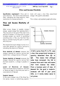
Graphical Representation Slope is not the same as elasticity, but they are related. All other things equal, an increase in price elasticity of demand will show up as a flattening of the demand curve. In the left-side diagram below, a small increase in price will produce a large decrease in demand. For this reason if demand is responsive to price changes (elastic), then you draw a flat demand curve. If on the other hand demand is unresponsive to price (inelastic), then the demand curve is steep. When demand is inelastic, a large increase in price will produce only a small decrease in demand (right-side diagram).

7

Responsive (elastic) demand

Unresponsive (inelastic) demand

The story is similar when we talk about price elasticity of supply. If quantity supplied is responsive to price changes, if supply is elastic, then the supply curve would be flat. An inelastic supply curve, meanwhile, would be represented by a steep supply curve.

Relationship between expenditures and elasticity Returning to the opening questions, many had to do with the link between elasticity and expenditures. The relationship between elasticity and expenditures can be described three ways - verbally, graphically, and algebraically - and all you need to do is master one of them. The words (with some algebra help) To understand the relationship between expenditures and elasticity let's look at some of the questions posed earlier. We'll begin with the Brazilian officials considering destroying some of the coffee crop. The impact of the decision depends upon the nature of the demand for coffee. If coffee drinkers need their coffee and they can be expected to pay whatever they need to pay to get their coffee fix, then demand is inelastic and we expect a reduction in coffee supply to increase price substantially as demanders compete for the smaller supply. The much higher price and slightly lower price means expenditures on coffee will rise - the increase in price more than compensating for the decreased quantity. It would be much the same for an official contemplating a fare change for the MBTA. The impact would depend upon the price elasticity of demand. If demand is unresponsive to price changes (inelastic), then fare reductions will not prompt many people to switch from cars to the subway, so the strategy of raising the fare would raise revenues. Elasticity of demand is also behind the higher airfares in large airline hub where a high percentage of flights are on a single airline. With fewer choices, elasticity of demand is low so airlines raise revenues by raising prices. As for the pricing of the fitness training, it was probably not an act of charity to lower the fitness fees for laid off workers. Maybe these fitness companies realized demand for their services is responsive to price, and that by lowering their price laid-off workers would continue to workout at their facilities, and when they get rehired they will pay the full fare. And let's close with one final example - the market for illegal drugs. It has been estimated that the own-price elasticity of demand for cocaine is -.28.viii With this information you should try to answer the following questions using the equations in this unit. 1. 2. 3.

If cocaine is legalized and its price drops 50%, what will happen to cocaine use? If drug policies are able to reduce supply by 10%, what will that do to the price of cocaine? If drug policies are able to reduce supply by 10%, what will it do to the revenue earned by the sellers?ix

Now don’t cheat and read on for the answers. Just identify the appropriate equations and fill in the values for the variables. 1.

Question 1: plug the knowns into the equation ep = %ΔQ/%ΔP and we get -.28 = %ΔQ/-50. I rearrange the terms and we get ΔQ = -.28*-50 = 14. With a 50% drop in price there will be a 14% increase in drug use.

8

2.

Question 2: plug the knowns into the equation ep = %ΔQ/%ΔP and we get -.28 = -10/%ΔP. I rearrange the terms and we get ΔP = -10/-.28 = 36 (A 10% reduction in supply will result in a 36% increase in price) 3. Question 3: plug the knows into the equation %ΔR = %ΔP + %ΔQ and we get %ΔR = 36 + -10 = 26% A 10% reduction in supply will generate a 26% increase in revenue earned by sellers. A summary of what we have just "proved" appears in the table below. If your goal is to raise revenue, then you should either reduce output or raise price if demand is inelastic, or raise output or lower price when demand is elastic. In the case of drugs, the policies to restrict supply will drive up price sharply and increase the revenues earned by the sellers.

1. 2.

Inelastic Demand | ep | < 1 Output and revenue are negatively related: to 1. raise revenue you would lower output Price and revenue are positively related: to 2. raise revenue you would raise price

Elastic Demand | ep | > 1 Output and revenue are positively related: to raise revenue you would raise output Price and revenue are negatively related: to raise revenue you would lower price

Incidence of tax What about taxes on booze and butts? Higher taxes on booze and butts also generate additional tax revenues because demand for these products is inelastic so an increase in price will not reduce demand enough to offset the higher tax. We'll still keep buying butts so the government gets more money. But be careful. This policy works at the national level, but will a decision by the Massachusetts legislature to raise tax rates on booze and butts to raise state tax revenue work? If demand for Massachusetts booze is elastic, because there are substitutes for Massachusetts booze (RI, CT, NH, and NY booze), the decision to raise prices will result in lower revenues. The moral here: do not be attached to the product. If demand is inelastic – if buyers’ demand is not much affected by price – then a tax will fall mostly on them because they ‘really’ want it and the suppliers will be able to raise prices to pay for the tax. If, however, demand is very responsive to price then suppliers will not be able to pass on the tax as a higher price so the firms will absorb the tax in a lower price.

The graphics (optional) Let's assume there is an increase in supply - the supply curve shifting to the right. Total revenue is by definition equal to the price times the quantity sold (P*Q). If you sell 20 units at a price of $5, total revenue will be $100 [$5*20]. In the diagrams below the initial situation is described by the solid supply curve (inner curve). The revenue earned from selling the output equals the areas A + B. After the increase in supply shifts the supply curve to the right (dashed line), revenue equals the area B + C. Revenue will increase as a result of the increase in supply if (area C) > (area A). In the diagrams below we see this happens when the demand curve is flat when demand is elastic. When demand is inelastic, revenue will decrease increase output or we decrease the price.

9

The algebra (optional) In this example you will be spared the derivation, although you should be able to derive the equations if you have some algebra skills. There are two important inputs into the algebra - the formula for the change in revenue (DR) and the formula for elasticity (ep).The first formula simply states that the change in revenue equals changes in price and changes in quantity, while the second defines elasticity as the ratio of percentage changes in quantity and price. ΔR = ΔQ*P + ΔP*Q ep = %ΔQ/%ΔP

or

%ΔR = %ΔQ + %ΔP

Now you can combine these equations and derive the relationship between the change in revenue (DR) and the change in price (DP), or quantity (DQ). These equations are specified in both change and percentage change terms. 1. 2.

ΔR = Q*(1+ep)* ΔP ΔR = P*(1+1/ep)* ΔQ

or in percentage terms 1. 2.

%ΔR = (1+ep)*% ΔP %ΔR =(1+1/ep)*% ΔQ

Now that you have made it through the tough part, we can interpret the results in the situation where demand is inelastic and where it is elastic by plugging in values for elasticity. You would use equations 1 and 3 if you were attempting to determine the impact of a price change on revenue while you would use equations 2 and 4 if you wanted to know about the impact of a change in output on revenue. For example, let us assume that demand elasticity is -2 [demand is elastic]. If we plug this value into equation 3, the term in parentheses becomes -1 [(1 + -2)] and we get the equation %DR = (-1)% DP. With a value of the term in the parentheses at -1, we find that revenue and price change in opposite directions. When demand is elastic, revenue and price change in opposite directions. If you wanted to raise revenue and demand was elastic, then you would lower the price. Similarly, if we plug the value -2 into equation 4 the term in the parentheses becomes .5 [(1 + 1/(-2)) = (1 - .5) = .5]. When demand is elastic you will find revenue and output moving in the same direction. If you wanted to raise revenue and demand were elastic, then you would increase supply.13 You should now have a good appreciation of the significance of elasticity to pricing and output decisions and the relationship between revenue and elasticity. You should also know why the low elasticity of demand for oil makes the US vulnerable to the supply restrictions of the OPEC nations.

10

Elasticity

i

"Yuppie Joblessness brings a new perk: Lid-Off Discounts," WSJ 12/5/2002 p 1 We focus on demand elasticities, but there is also the Supply elasticity that is a measure of how supply responds to a change in price. Definition: Price elasticity of supply = the percentage change in supply generated by a one percent change in price. Formula: Price elasticity of supply = eps = %ΔQs/%DΔP This formula simply describes a relationship between three unknowns - the price elasticity of supply (eps), the percentage change in supply (%ΔQs) and the percentage change in price (%ΔP). All you need to do is use the formula to solve problems, and you may recall from your algebra courses, to solve for one unknown you need to have the values for the other two unknowns. Let's assume you have studied the supply of oil in the world and realize that every time the price of oil rises 10 percent (%DΔP) the supply of oil rises 15 percent (%ΔQs). If you look at the equation you will see the unknown is the price elasticity of supply (eps). So let's plug it into the equation. eps = %ΔQs/%ΔP = 15/10 = 1.5. What you have found is that the elasticity of supply is 1.5, which means that for every 1 percent increase in the price there will be a 1.5 percent increase in supply. Now assume you know that the price elasticity of supply is 1.5 and you need to generate a 9 percent increase in supply. What would be the price increase necessary to generate the increased supply? With a little bit of algebra you isolate the unknown (percentage change in price) on the left side of the = sign and then plug in the known values. %ΔP = %ΔQs/eps = 9/1.5 = 6 You have shown that to get the 9 percent increase in supply you would need to increase price by 6 percent with a price elasticity of supply equal to 1.5. And now that you are on a roll, what would happen to supply if the price elasticity of supply were 2 and the price decreased by 10 percent? Isolating the unknown (%DQ) and then plugging in the value for the two knowns you find that a 10 percent decrease in the price would reduce supply (negative sign) by 20 percent when the supply price elasticity is 2. %ΔQ = eps *%ΔP= 2*-10 = -20 iii The data on SUV sales can be found in Nick Bunkley, "An SUV Traffic Jam," NYT August 13, 2008, while the gas price data came from the Energy Information Agency. You could also determine the change in the price of computers necessary to increase demand for software by 8 percent if the cross-price elasticity is -2. Following the same process you would isolate the unknown (%ΔPo) and then plug in the value for the two knowns. The 8 percent increase in the demand for the software would require a 4 percent decrease in income if the cross-price elasticity were -2. %ΔPo =%ΔQ/ePo= 8/-2 = -4 iv The table is from a Mackinac Center policy research paper. v Hackl & Westlund, Journal of Econometrics 1996. vi An example of the impact of time is evident in Samuel R. Staley's review of Richard Voith's article, "The Long-Run Elasticity of Demand for Commuter Rail Transportation," Journal of Urban Economics (1991), pp. 360-72. According to Staley, "In the long run, demand is strikingly elastic with respect to own price (-1.59), the variable cost of an auto trip (2.69), and the fixed cost of auto ownership (1.13)." ... we find that ridership is more than twice as elastic in the long run as in the short run. Ridership on SEPTA, which is price inelastic in the short run, is price elastic in the long run. The characteristics of service such as frequency and speed of trains, and alternative transportation prices, have significant effects on ridership, which are substantially larger in the long run than in the short run." vii The following table summarizes the results of numerous studies reported in the article. ii

Researcher/s Carver and Boland Agthee and Billings Martin et al Hanke and de Mare Gallagher et al Boistard Thomas and Syme Veck and Bill3

Date 1969 1974 1976 1971 1972/3 & 1976/7 1985 1979 1998

Location Washington D.C. Tucson, Arizona Tucson, Arizona Malmo, Sweden Toowoonba, Queensland France Perth, Australia. Alberton & Thokoza, South Africa

Price Elasticity -0,1 -0,18 -0,26 -0,15 -0,26 -0,17 0,18 -0,17

Saffer & Chaloupka, "The demand for illicit drugs," Economic Enquiry, July 1999 pp. 401-411 Question 1: plug the knowns into the equation ep = %ΔQ/%ΔP and we get -.28 = %ΔQ/-50. I rearrange the terms and we get DQ = -.28*-50 = 14 (there will be a 14% increase in drug use) Question 2: plug the knows into the equation ep = %ΔQ/%ΔP and we get -.28 = -10/%ΔP. I rearrange the terms and we get DP = 10/-.28 = 36 (there will be a 36% increase in price

viii ix

11

Question 3: plug the knows into the equation %ΔR = %ΔP + %ΔQ and we get %ΔR = %Δ36 + -10 = 26% ( there will be a 26% increase in revenue earned by sellers) If you think you really have it down, let's try one more problem based on the article "ESTIMATION OF THE RESIDENTIAL PRICE ELASTICITY OF DEMAND FOR WATER BY MEANS OF A CONTINGENT VALUATION APPROACH." where the elasticity of demand was estimated to be approximately -.2. Given this elasticity of demand, what would have to happen to the revenue earned from selling water if you needed to cut demand by 20%? We need to go back to our two equations (1) %ΔR = %ΔP + %ΔQ (2) ep = %ΔQ/%ΔP We have two equations with four unknowns, which would be a problem except for the fact we have values for two of the unknowns. We know ep = -.2 and that %DQ = -20 because this is the target. Let's plug them into the equations (1) %ΔR = %ΔP + -20 (2) -.2 = -20/%ΔP Equation 2 can be rewritten so we can solve for the change in P necessary to reach the demand reduction. %ΔP = -2/-.2 = 100 This means there will need to be a 100% increase in the price of water to reach the desired 20% reduction in demand. This information can then be plugged into the first equation and you find revenue will increase by 80%. (1) %ΔR = 100 - 20 = 80

12