Chapter 6
Determinants of the Real Exchange Rate In the previous chapter, we saw that among industrialized countries real interest rate differentials can be explained, to a large extent, by expected changes in the real exchange rate. Figure 2.3 of the Frankel article (Das reader, p. 34) shows the dollarpound real exchange rate from 1869 to 1987. The dollar-pound real exchange rate, e$/£ , is given by E $/£ P U K /P U S , where E $/£ is the dollar-pound nominal exchange rate (i.e., the dollar price of one pound), P U K is the price level in the U.K., and P U S is the price level in the U.S. Thus, e$/£ is the relative price of a consumption basket in the U.K. in terms of consumption baskets in the United States. The figure shows that the real exchange rate varied a lot from year to year and that deviations of the real exchange rate from its mean value were highly persistent. This means that PPP (i.e., P U S = E $/£ P U K ) does not hold. However, the real exchange rate seems to fluctuate around a constant mean. For example, the real exchange rate in 1987 is almost the same as the real exchange rate in 1869. Therefore, over very long horizons, PPP is a somewhat useful approximation to actual real exchange rate behavior. If PPP holds over the long run, then it must be the case that %∆E = %∆P − %∆P ∗
(6.1)
where %∆E, %∆P , and %∆P ∗ denote, respectively, the percentage change in the nominal exchange rate (or rate of nominal exchange rate depreciation), the percentage change in the domestic price level (or the rate of domestic inflation), and the percentage change in the foreign price level (or the rate 93
94
S. Schmitt-Groh´e and M. Uribe
of foreign inflation) over a long period of time. Figure 10-6 on p. 316 in the Sachs and Larrain textbook shows a scatterplot of average rates of nominal exchange rate depreciation versus average rates of inflation between 1965 and 1985 for a number of countries. Equation (6.1) states that if PPP holds over the long run, then the points on the scatterplot should lie on a line with slope equal to 1 and an intercept of −%∆P ∗ . Because the graph shows changes in dollar exchange rates, the intercept should be the U.S. inflation rate. The figure shows that this relation is quite accurate, especially for high inflation countries: countries with high average exchange rate depreciations were countries that experienced high average inflation rates, and countries whose currency did not depreciated much vis-`a-vis the U.S. dollar tended to have much lower average inflation rates. In the two-period model we developed in chapters 2 and 3, there is a single traded good. Thus, under the maintained assumption of free international trade, purchasing power parity obtained, that is, e = EP ∗ /P = 1. Why is the prediction of our theoretical model that PPP holds not right? One reason is that in reality, contrary to what is assumed in the model, not all goods are tradable. Examples of such goods are haircuts, Big Macs, real estate, and other services. For these goods transport costs are so large relative to the production cost that they can never be traded internationally at a profit. Such goods and services are called nontradables. In general, nontradables make up a significant share of a country’s output, typically above 50 percent. The existence of nontradables allows for systematic violations of PPP. The price index P is an average of all prices in the economy. Thus, it depends on both the prices of nontradables and the prices of tradables. But the prices of nontradables are determined entirely by domestic factors, so one should not expect the law of one price to hold for this type of goods. Other things equal, a rise in the price of nontradables in the domestic economy can increase a country’s aggregate price level relative to the foreign price level. To see this, let PT and PN denote the domestic prices of tradables and nontradables, respectively, and let PT∗ and PN∗ denote the corresponding foreign prices. For traded goods the law of one price should hold, that is, PT = EPT ∗ , but for nontraded goods it need not PN �= EPN ∗ . Suppose the price level, P , is constructed as follows: P = φ(PT , PN )
International Macroeconomics, Chapter 6
95
where φ is increasing in PT and PN and homogeneous of degree one.1 The price level P is an average of individual prices. The assumption that φ(·, ·) is homogeneous of degree one ensures that, if all individual prices increase by, say, 5%, then P also increases by 5%. Given the way in which the price level is constructed, the real exchange rate, e, can be expressed as e = = = =
EP ∗ P Eφ(PT∗ , PN∗ ) φ(PT , PN ) EPT∗ φ(1, PN∗ /PT∗ ) PT φ(1, PN /PT ) φ(1, PN∗ /PT∗ ) φ(1, PN /PT )
(6.2)
So the real exchange rate should depend on the ratio of nontraded to traded prices in both countries. The real exchange rate is greater than one (or the price of the foreign consumption basket is higher than the price of the domestic consumption basket) if the relative price of nontradables in terms of tradables is higher in the foreign country than domestically. Formally, e > 1 if
∗ PN PT∗
>
PN PT .
It is straightforward to see from this inequality that e can increase over time if the price ratio on the left-hand side increases over time more than the one on the right hand side. When talking about a particular country pair, it is useful to define a bilateral real exchange rate. For example, the dollar-mark real exchange rate is given by e$/DM =
E $/DM P Germany Price of German goods basket = P U.S. Price of US goods basket
Suppose e$/DM increases, then the price of the German goods basket in terms of the U.S. goods basket increased, and we say that the dollar real exchange rate vis-`a-vis the German mark depreciated, because it takes now more U.S. goods baskets to purchase one German goods basket. At this point, a word of caution about semantics is in order. Economists use the term real exchange rate loosely. The term real exchange rate is 1
A function f (x, y) is homogenous of degree one if f (x, y) = λf (x/λ, y/λ).
96
S. Schmitt-Groh´e and M. Uribe
sometimes used to refer to EP ∗ /P and sometimes to refer simply to PT /PN . A real exchange rate appreciation means that either PT /PN falls or that EP ∗ /P falls, depending on the concept of real exchange rate being used. Similarly, a real exchange rate depreciation means that either PT /PN goes up or that EP ∗ /P goes up. Next we turn to an analysis of the determinants of real exchange rates. We begin by studying a theory that explains long-run variations in bilateral real exchange rates.
6.1
Productivity Differentials and Real Exchange Rates: The Balassa-Samuelson Model
According to the Balassa-Samuelson model deviations from PPP are due to cross-country differentials in the productivity of technology to produce traded and nontraded goods. In this section we study a simple model that captures the Balassa-Samuelson result. Suppose a country produces 2 kinds of goods, traded goods, QT , and nontraded goods, QN . Both goods are produced with a linear production technology that takes labor as the only factor input. However, labor productivity varies across sectors. Specifically, assume that output in the traded and nontraded sectors are, respectively, given by QT = aT LT
(6.3)
QN = aN LN ,
(6.4)
and
where LT and LN denote labor input in the traded and nontraded sectors. Labor productivity is defined as output per unit of labor. Given the linear production technologies, we have that labor productivity in the traded sector is aT and in the nontraded sector is aN .2 In the traded sector, a firm’s profit is given by the difference between revenues from sales of traded goods, PT QT , and total cost of production, 2
There are two concepts of labor productivity: average and marginal labor productivity. Average labor productivity is defined as output per worker, Q/L. Marginal labor productivity is defined as the increase in output resulting from a unit increase in labor input, holding constant all other inputs. More formally, marginal labor productivity is given by the partial derivative of output with respect to labor, ∂Q/∂L. For the linear technologies given in (6.3) and (6.4), average and marginal labor productivities are the same.
International Macroeconomics, Chapter 6
97
wLT , where w denotes the wage rate per worker. That is, profits in the traded sector = PT QT − wLT Similarly, in the nontraded sector we have profits in the nontraded sector = PN QN − wLN We assume that there is perfect competition in both sectors and that there are no restrictions on entry of new firms. This means that as long as profits are positive new firms will have incentives to enter, driving prices down. Therefore, in equilibrium, prices and wages must be such that profits are zero in both sectors, PT QT = wLT PN QN = wLN Using the production functions (6.3) and (6.4) to eliminate QT and QN from the above two expressions, the zero-profit conditions imply PT aT = w and PN aN = w. Combining these two expressions to eliminate w yields aN PT = . PN aT
(6.5)
This expression says that the relative price of traded to nontraded goods is equal to the ratio of labor productivity in the nontraded sector to that in the traded sector. To understand the intuition behind this condition suppose that aN is greater than aT . This means that one unit of labor produces more units of nontraded goods than of traded goods. Therefore, producing 1 unit of nontraded goods costs less than producing 1 unit of traded goods, and as a result nontraded goods should be cheaper than traded goods (PN /PT < 1). According to equation (6.5), a period in which labor productivity in the nontraded sector is growing faster than labor productivity in the traded sector will be associated with real exchange rate depreciation (i.e., with PT /PN rising).
98
S. Schmitt-Groh´e and M. Uribe
In the foreign country, the relative price of tradables in terms of nontradables is determined in a similar fashion, that is, PT∗ a∗N = , PN∗ a∗T
(6.6)
where PT∗ /PN∗ denotes the relative price of tradables in terms of nontradables in the foreign country, and a∗T and a∗N denote the labor productivities in the foreign country’s traded and nontraded sectors, respectively. To obtain the equilibrium bilateral real exchange rate, e = E P ∗ /P , combine equations (6.2), (6.5) and (6.6): e=
φ(1, a∗T /a∗N ) φ(1, aT /aN )
(6.7)
This equation captures the main result of the Balassa-Samuelson model, namely, that deviations from PPP (i.e., variations in e) are due to differences in relative productivity growth rates across countries. In particular, if in the domestic country the relative productivity of the traded sector, aT /aN , is growing faster than in the foreign country, then the real exchange rate will appreciate over time (e will fall over time), this is because in the home country nontradables are becoming relatively more expensive to produce than in the foreign country, forcing the relative price of nontradables in the domestic country to grow at a faster rate than in the foreign country. The relative price of traded goods in terms of nontraded goods, PT /PN , can be related to the slope of the production possibility frontier as follows. Let L denote the aggregate labor supply, which we will assume to be fixed. Then the resource constraint in the labor market is L = LN + LT Use equations (6.3) and (6.4) to eliminate LN and LT fro this expression to get L = QN /aN + QT /aT . Now solve for QN to obtain the following production possibility frontier (PPF) QN = aN L −
aN QT aT
Figure 6.1 plots the production possibility frontier. The slope of the PPF is aN dQN =− dQT aT Combining this last expression with equation (6.5), it follows that the slope of the PPF is equal to −PT /PN .
International Macroeconomics, Chapter 6
99
Figure 6.1: The production possibility frontier (PPF): the case of linear technology QN aN L ← slope = − a /a =−P /P N
T
aT L
6.1.1
T
N
QT
Application: the real dollar-yen exchange rate, 19501995
Figure 15-5 in the Krugman and Obstfeld textbook (p. 428) shows the dollaryen real exchange rate from 1950 to 1995. Over this period, the yen appreciated steadily versus the U.S. dollar, or the dollar depreciated vis-` a-vis the yen in real terms (e$/U = E $/U P J /P U S went up). For example, in 1970 e$/U was 100 and in 1995 it was about 300. What does the Balassa-Samuelson model have to say about this real depreciation of the dollar versus the yen? Recall that the bilateral dollar-yen real exchange rate is given by e$/U =
φ(1, PNJ /PTJ ) φ(1, PNU S /PTU S )
It follows from this relationship that the ratio of prices of traded to nontraded goods must have changed at different rates in the two countries. Because e$/U went up over time the percentage change in (PNJ /PTJ ) must have been larger than the percentage change in same ratio for the United States. Empirical studies have documented that over the period considered in the United States as well as in Japan, productivity in the traded sector grew faster than productivity in the nontraded sector. However, in Japan productivity growth in the traded sector relative to the nontraded sector was found to be much higher than in the United States. According to the Balassa-Samuelson model, this would imply that PN /PT rose more in Japan
100
S. Schmitt-Groh´e and M. Uribe
than it did in the United States. So the model implies that the U.S. real exchange rate should have depreciated, that is, e$/U should have gone up, which is exactly what was observed.
6.1.2
Application: Deviations from PPP observed between rich and poor countries
Table 6.1 shows the bilateral real exchange rate for a number of countries Table 6.1: The real exchange rate of rich and poor countries, 1980
Country Bangladesh Ethiopia India Pakistan Unites States West Germany Switzerland Sweden
Real Exchange Rate 4.2 2.3 2.6 3.3 1.0 0.7 0.6 0.7
Source: Sachs and Larrain, table 21-4, p. 679.
vis-`a-vis the United States. Countries are divided into two groups, poor countries and rich countries. The real exchange rate for a given country, say India, vis-` a-vis the United States, erupee/$ is given by E rupee/$ P U S /P I , rupee/$ is the rupee/dollar nominal exchange rate defined as the where E price of one dollar in terms of rupee, P U S is the price level in the U.S., and P I is the price level in India. The table shows that the real exchange rate in poor countries, epoor/U S , is typically greater than that in rich countries, erich/U S . For example, the Bangladesh/U.S. real exchange rate in 1980 was 4.2, but Switzerland’s real exchange rate vis-` a-vis the dollar was only .6. This means that in 1980 a basket of goods in Switzerland was 7(=4.2/.6) times as expensive as in Bangladesh. How can we explain this empirical regularity? Note that epoor/U S = erich/U S
E poor/U S P U S P poor E rich/U S P U S P rich
=
E poor/U S P rich E poor/rich P rich = = epoor/rich P poor E rich/U S P poor
International Macroeconomics, Chapter 6
101
Using equation (6.2), epoor/rich can be expressed as epoor/rich =
φ(1, PNrich /PTrich ) φ(1, PNpoor /PTpoor )
Finally, using the Balassa-Samuelson model, to replace price ratios with relative labor productivities (equation (6.6)), we get epoor/rich =
rich φ(1, arich T /aN ) φ(1, apoor /apoor T N )
Productivity differentials between poor and rich countries are most extreme rich > apoor /apoor . So the in the traded good sector, implying that arich T /aN T N observed relative productivity differentials can explain why the real exchange rate is relatively high in poor countries. The Balassa-Samuelson framework is most appropriate to study long-run deviations from PPP because productivity differentials change slowly over time. However, we also observe a great deal of variation in real exchange rates in the short run. The next two sections study sources of short-run deviations from PPP.
6.2
Trade Barriers and Real Exchange Rates
In the previous section, deviations from PPP occur due to the presence of nontradables. In this section, we investigate deviations from the law of one price that may arise even when all goods are traded. Specifically, we study deviations from the law of one price that arise because governments impose trade barriers, such as import tariffs, export subsidies, and quotas, that artificially distort relative prices across countries. Consider an economy with 2 types of traded goods, importables and ∗ , and the world price exportables. Let the world price of importables be PM ∗ of exportables be PX . Assume for simplicity that there are no nontradable goods. In the absence of trade barriers, PPP must hold for both goods, that is, the domestic prices of exportables and importables must be given by PX = EPX∗ and ∗ , PM = EPM
102
S. Schmitt-Groh´e and M. Uribe
where E denotes the nominal exchange rate defined as the domestic currency price of one unit of foreign currency. The domestic price level, P , is an average of PX and PM . Specifically, assume that P is given by P = φ(PX , PM ), where φ(·, ·) is an increasing and homogeneous-of-degree-one function. A similar relation holds in the foreign country ∗ P ∗ = φ(PX∗ , PM )
The bilateral real exchange rate, e = EP ∗ /P , can then be written as e=
∗ ) ∗ ) Eφ(PX∗ , PM φ(EPX∗ , EPM φ(PX , PM ) = = = 1, φ(PX , PM ) φ(PX , PM ) φ(PX , PM )
where the second equality uses the fact that φ is homogeneous of degree one and the third equality uses the fact that PPP holds for both goods. Consider now the consequences of imposing a tariff τ > 0 on imports in the home country. The domestic price of the import good therefore increases by a factor of τ , that is, ∗ . PM = (1 + τ )EPM
The domestic price of exportables is unaffected by the import tariff. Then the real exchange rate becomes e=
∗ ) ∗ ) φ(EPX∗ , EPM Eφ(PX∗ , PM = ∗ ∗ ) < 1, φ(PX , PM ) φ(EPX , (1 + τ )EPM
where the inequality follows from the fact that φ(·, ·) is increasing in both arguments and that 1 + τ > 1. This expression shows that the imposition of import tariffs leads to an appreciation of the real exchange rate as it makes the domestic consumption basket more expensive. Therefore, one source of deviations from PPP is the existence of trade barriers. One should expect that a trade liberalization that eliminates this type of trade distortions should induce an increase in the relative price of exports over imports goods so e should rise (i.e., the real exchange rate should depreciate).3
3
How would the imposition of an export subsidy affect the real exchange rate?