International Journal of Economics and Finance; Vol. 4, No. 8; 2012 ISSN 1916-971X E-ISSN 1916-9728 Published by Canadian Center of Science and Education

The Determinants of Real Exchange Rate in Nigeria Victor E. Oriavwote1 & Dickson O. Oyovwi2 1

Department of Arts and Social Sciences, Delta State Polytechnic, Otefe-Oghara, Delta State, Nigeria

2

Department of Economics, College of Education, Warri, Delta State, Nigeria

Correspondence: Victor E. Oriavwote, Department of Arts and Social Sciences, Delta State Polytechnic, Otefe-Oghara, Delta State, Nigeria. Tel: 80-35-814-123. E-mail: [email protected] Received: May 20, 2012 doi:10.5539/ijef.v4n8p150

Accepted: June 12, 2012

Online Published: July 11, 2012

URL: http://dx.doi.org/10.5539/ijef.v4n8p150

Abstract In this paper, an attempt is made to investigate the determinants of the real exchange rate in Nigeria. The objective of the study has been to present a dynamic model of real exchange rate determination and empirically test the implications of changes in possible determinants of the real exchange in Nigeria. With data covering 1970-2010, the parsimonious ECM result shows amongst others that the ratio of government spending to GDP, terms of trade and technological progress are not important determinants of the real effective exchange rate in Nigeria. The result showed that capital flow, price level and nominal effective exchange rate are important determinants of the real effective exchange rate in Nigeria. The paper suggests that the Dutch Disease syndrome holds in Nigeria. The Johansen cointegration test suggests a long relationship among the variables. It is thus recommended amongst others that policies have to be put in place to stabilize the problem of inflation. Keywords: Real Exchange Rate, cointegration, parsimonious Error Correction model, Dutch disease 1. Introduction The relationship between a country’s exchange rate and economic growth is a crucial issue from both the descriptive and policy prescription perspectives. As Edwards (1994) puts it “it is not an overstatement to say that real exchange rate behaviour now occupies a central role in policy evaluation and design”. A country’s exchange rate is an important determinant of the growth of its cross-border trading and it serves as a measure of its international competitiveness (Bah and Amusa, 2003). The real exchange rate, in particular, defined as the relative price of foreign goods in terms of domestic goods, is of greater significance, as it is an important relative price signalling inter-sectoral growth in the long run and acts as a measure of international competitiveness. In other words, the real exchange rate plays a crucial role in guiding the broad allocation of production and spending in the domestic economy between foreign and domestic goods. The role of international trade in economic development has been acknowledged worldwide. This is because it provides opportunities to expand both the production possibilities and consumption basket available to the people (Adewuyi, 2005). The Nigerian government has over the years engaged in international trade and has been designing trade and exchange rate policies to promote trade (Adewuyi, 2005). Although a number of exchange rate reforms have been carried out by successive governments, the extent to which these policies have been effective in promoting export has remained unascertained. This is because despite’ government efforts, the growth performance of Nigeria non-oil export has been very slow. It grew at an average of 2.3% during the 1960 -1990 period, while its share of total export declined from about 60% in 1960 to 3.0% in 1990 (Ogun, 2004). Looking at the sectoral contribution to non-oil export in the period before the introduction of the Structural Adjustment Programme (SAP) (1975-1985), it can be seen that agricultural sector contributed about 4.0% and 67.0% to total export and non-oil export respectively (Ogun, 2004). The shares of manufacturing ‘sector in these categories of exports are about 1.0 and 12.0% respectively during that same period (Ogun, 2004). Overvalued RER has reduced profit in tradable good sector, thereby reducing investment in this sector. This has negative implications on exports and hence the trade balance. Persistent overvaluation of the RER may also lead to currency crisis (Xiaopu, 2002). The growing overvalued exchange rate that took off in Sub-Sahara Africa in the early 1980s contributed to the poor performance of the current account balances in the Region. Despite various efforts by the government to maintain exchange rate stability (as well as avoiding its fluctuations and misalignment) in the last two decades, the naira exchange rate to the American dollar depreciated throughout the 150

www.ccsenet.org/ijef

International Journal of Economics and Finance

Vol. 4, No. 8; 2012

1980s. For example, the naira depreciated from N0.61 in 1981 to N2.02 in 1986 and further to N8.03 in 1990. Although the exchange rate became relatively stable in the mid 1990s, it depreciated further to N120.97, N129.36 and N133.50 in 2002, 2003 and 2004 respectively (Obadan, 2006). Thereafter, the exchange rate appreciated to N132.15, N128.65, N125.83 and N118.57 in 2005, 2006, 2007 and 2008 respectively (Central Bank of Nigeria, 2008). Some have attributed the recent deprecation to the decline in the nation’s foreign exchange reserves, but others argue that the activities of speculators and banks are responsible for the recent decline in the value of the naira. Also, the recent global economic meltdown is forcing some banks to engage in ‘round-tripping’, a situation in which banks buy foreign exchange from the Central Bank of Nigeria (CBN) and sell to parallel market operators at prices other than the official prices. These practices have resulted in fluctuation and misalignment in the real exchange rate. In his view, Obadan (2006) summed up the factors that led to the misalignment of the real exchange rate in Nigeria to include weak production base, import dependent production structure, fragile export base and weak non-oil export earnings, expansionary monetary and fiscal policies, inadequate foreign capital inflow, excess demand for foreign exchange relative to supply, fluctuations in crude oil earnings, unguided trade liberalization policy, speculative activities and sharp practices (round tripping) of authorized dealers. Others include over reliance on imperfect foreign exchange market, heavy debt burden, weak balance of payments position and capital flight. The important question is ‘what are the determinants of the real exchange rate in Nigeria, taking into account both short run (actual) and long run determinants’? The objective of this study is thus to present a dynamic model of real exchange rate determination and empirically test the implications of changes in possible determinants of the real exchange rate in Nigeria. The sub-objectives include: to assess the impact of terms of trade on the real exchange rate in Nigeria; to establish the extent to which the openness of the economy affects the real exchange rate in Nigeria; to analyze the relationship between the variation in capital flow and the real exchange rate in Nigeria; to ascertain the impact of nominal devaluation on the real exchange rate; to assess the relationship between fiscal policy and the real exchange rate and to assess the relationship between changes in the general price level and the real exchange rate in Nigeria. Other than this introductory section, the rest of the paper is divided into three sections. The first section focuses on literature review which is made up of empirical literature and theoretical literature. The second deals with econometric procedure and the last section concludes this paper. 2. Literature Review This is divided into empirical literature and theoretical literature 2.1 Empirical Literature Edwards (1989) pioneered the fundamentals models of the determination of real exchange rates for developing countries. Edwards started by developing a theoretical model of the real exchange rate determination and then estimated its equilibrium value for a panel of 12 developing countries (Brazil, Columbia, El Salvador, Greece, India, Israel, Malaysia, Philippines, South Africa, Sri Lanka, Thailand and Yugoslavia) using conventional cointegration tests on time series data. To analyse the relative importance of real and nominal variables in the process of real exchange rate determination in the short and long run, he used the following partial adjustment model: RER = v(terms of trade, government consumption, capital controls, exchange controls, technical progress, domestic credit, real growth, nominal devaluation). The study found that in the long run only real variables affect the long run equilibrium real exchange rate. In the short run, however, real exchange rate variability was explained by both real and nominal factors. Obadan (1994) formulated a simple econometric model for Nigeria and empirically estimated it together with a random walk model of the real exchange rate determination. Both models were estimated in log-linear forms using the two-stage least squares regression methodology and data for the period 1970-1988. Although this study failed to test variables for stationarity and did not estimate the equilibrium real exchange rate, it found that both structural and short run factors were important determinants of variations in prevailing bilateral real exchange rates and multilateral real effective exchange rates. The study found that the most important factors were international terms of trade, net capital inflows, nominal exchange rate policy and monetary policy. Mungule (2004) investigated the determinants of real exchange rate in Zambia. He used the real exchange rate as a function of terms of trade, capital inflow, closeness of the economy and excess supply of domestic credit. Using the cointegration technique, he discovered that the REER and the fundamental determinants have a long run equilibrium relationship. Ogun (2004) examined the impact of real exchange rate on growth of non-oil export in Nigeria. Specifically, he analyzed the effects of real exchange rate misalignment and volatility on the growth of non oil exports. He employed the standard trade theory model of determinants of export growth and two different measures of real exchange rate misalignment, one of which 151

www.ccsenet.org/ijef

International Journal of Economics and Finance

Vol. 4, No. 8; 2012

entailed deviations of purchasing power parity (PPP) and the other was model based estimation of equilibrium real exchange rate. He reported that, irrespective of the alternative measures of misalignment adopted, both real exchange rate misalignment and volatility adversely affected growth of Nigeria’s non-oil export. This study on the determinants of the real exchange rate in Nigeria however differs from most of the works reviewed because a critical examination of these works, particularly those from Nigeria, showed that most of them did not take into account the time series characteristics of the macroeconomic data used. Also most of the works also used the traditional methods of estimation such as the OLS or Two Stage Least Squares 2SLS. They did not also take into account recent experiences of the real exchange rate particularly from the time of the Structural Adjustment Programme (SAP). In this study, we have therefore adopted a cointegration approach to analyze the determinants and behaviour of real exchange rate in Nigeria. Moreover, the study provides a better assessment because it covers a wider duration of 39 years of inter-temporal change in the behaviour of economic agents taking as an aggregate. The review of empirical literature also showed that very few studies have been carried out in Nigeria in this area. The empirical works revealed that while the real exchange rate is calculated using the nominal exchange rate and the price level, the nominal exchange rate has been included in models of real exchange rate, but the price level has not been included in these models. Thus, one of the departure points of this study from the previous studies is that it includes the direct effects of the price level on the real exchange rate. This study adopts the Mungule (2004) model. However, unlike the Mungule’s model, the study uses the degree of openness instead of closeness. The study, unlike Mungule’s model also includes the nominal effective exchange rate as an explanatory variable. This research also included the impact of fiscal policy, through government expenditure which was not included in Mugule (2004) model. The impact of technological progress on the real exchange rate was also taken care of in this model. Mungule studied the Zambian economy, but this study is on the Nigerian economy and covered the period between 1970 to 2008. 2.2 Theoretical Literature Edwards (1989) model assumes a small, open economy, which produces and consumes two goods-tradables and nontradables. Importables and exportables are aggregated into one tradable category. The government sector consumes both tradables and nontradables and finances its expenditures by non-distortionary taxes and domestic credit creation. The country holds both domestic money and foreign money. At a later stage of the study it is assumed that there are no capital controls, and that there are some capital flows in and out of the country. The nominal exchange rate of the economy is fixed with a basket of currencies of its major trading partners. It is also assumed that there is a tariff on imports. The price of tradables in terms of foreign currency is fixed and equal to unity, that is, PT = 1. Finally, perfect foresight is assumed in this model. The model is represented by the following equations: Portfolio Decisions B = M + FM

(1)

b = m + fm where b = B/E, m = M/E, fm = FM/E

(2)

FM  0

(3)

Demand Side c = E*Pt/PNT

CT/e0

CT = CT(e, b); CNT = CNT(e, b);

CNT/e>0; CNT/b>0

(4) (5) (6)

Supply Side ST = ST(e);

ST/e0; n/PT>0, n/>0 153

(19)

www.ccsenet.org/ijef

International Journal of Economics and Finance

Vol. 4, No. 8; 2012

Equilibrium in the external sector requires that m = 0.The following equation of m can be derived from earlier equations as: m = {ST(e) - CT (e, b)} - KA + gNT - t/E

(20)

When government expenditures are fully financed with taxes, the R = 0 will coincide with the m = 0 From Equations 18 and 19 it is possible to find an equilibrium relation between e, b, gNT and . ERER = e* = x (b, gNT, PT and )

(21)

where, x/b < 0; x/gNT < 0; x/PT > 0; x/ < 0 A rise in domestic money, m, in terms of foreign currency, results in higher real wealth and a current account deficit. To bring back equilibrium, real wealth, the price of nontradabes will rise (Equation 18). Thus, an increase in real assets increases the price of nontradebles and causes the RER to appreciate in order to ensure long run equilibrium. Increases in government expenditure on nontradables (gNT) have the same effect on the ERER. A rise in the price of tradables causes the RER to depreciate, given, that the price of nontradablcs and the nominal exchange rate remain constant. However, if the increase in the PT increases export earnings, and is spent on the nontradable sector, the demand for and price of nontradables will increase more than the PT causing a RER appreciation. The total effect of an import tariff depends on the initial expenditure on domestic nontradables and importables. An increase in the tariff on importables worsens the current account by increasing import bills, lowers the demand for tradables, raises the demand and price for nontradables and tends to lead to an appreciation of the long run real exchange rate. But if an increase in tariff worsens the current account balance without any substitution effects, it will increase the composite PT alone and may depreciate the real exchange rate. It is therefore, possible to observe, simultaneously, a real depreciation and a worsening of the current account. So the increase in the PT and changes in trade policies can have either positive or negative impacts on the RER. Equation 20 indicates that the long run equilibrium RER is a function of real variables only. The value of real assets, government consumption, price of tradables and trade restrictions in this equation are normally influenced by changes in other real variables such as terms of trade (TOT) shocks, changes in government expenditure, technological progress, and changes in trade and capital restrictions. Changes in these real variables can cause the actual RER to deviate from its equilibrium level. However, changes in nominal variables, such as domestic credit expansion, and changes in the values of nominal exchange rate, also affect the path of the actual RER in the short run. 3. Econometric Procedure To guard against the possibility of estimating spurious relationships in the presence of some nonstationary variables, estimation is performed using a general-to-specific Hendry-type error correction modelling (ECM) procedure. This procedure begins with an over-parameterised autoregressive distributed lag (ADL) specification of an appropriate lag. The consideration of the available degrees of freedom and type of data determine the decision on lag length. With annual data, one or two lags would be long enough, while with quarterly data a maximum lag of four can be taken. Under this ECM procedure, the long run relationship is embedded within the dynamic specification. Based on this theoretical background and on data availability, this study estimates the following relationship: REERt=0+1TOT + 2OPEN + 3GSPGDP + 4NEER+5TECHPROt+6RGDPt +B7P+ B8CAPFLGDP +t where the following notation has been used: REER

= real effective exchange rate,

CAPFLGDP

= ratio of capital flow to Gross Domestic Product(GDP)

TOT

= terms of trade,

OPEN

= an indicator of the degree of openness,

GSPGDP

= the ratio of government spending (fiscal policy) to GDP,

TECHPRO

= measure of technological progress (Balassa-Samuelson effect),

NEER

= nominal effective exchange rate policy

RGDP

=

Real Gross Domestic Product

P

= rate of inflation 154

www.ccsenet.org/ijef



International Journal of Economics and Finance

Vol. 4, No. 8; 2012

= error term.

3.1 Definition and Sources of Variables Conventionally, proxies have to be found for variables without time series data. Their construction is explained below. REER: The real effective exchange rate of the naira, measured in foreign currency terms, thus an increase in this variable indicates an appreciation of the naira. The data was gotten from the World Bank Indicators-Nigeria-Exchange Rates and prices, 2010. OPEN: This is a measure of the degree of openness. It is defined as the ratio of the sum of imports and exports of goods and services to GDP. Several other proxies ranging from the ratio of the tariffs to GDP to the ratio of tariff revenues to imports have been used, but this is the proxy that has been used by the majority of the studies (see Edwards, 1994, Aron, Elbadawi and Khan, 1997, Mkenda, 2001 and MacDonald and Ricci, 2003).The ata was gotten from the authors’ computation. TECHPRO: Technological progress data is also not readily available, so we have to find a proxy for it. We follow Edwards (1994) and MacDonald (1998) and use real GDP growth rate. The data was gotten from the authors’ computation. P: Represents the domestic rate of inflation. Excess domestic credit increases the price level which lead to an appreciation of the real exchange rate. The data was gotten from the CBN statistical bulletin, 2010. CAPFLGDP: This is taken to be the ratio of capital to the GDP. The data was gotten from the CBN statistical bulletin and authors’ computation. NEER: Data for the Nominal Effective Exchange Rate was gotten from the CBN statistical bulletin. TOT: Data on terms of trade was gotten from the World Bank development indicators for Africa. RGDP: Data on the Real Gross Domestic Product was gotten from CBN statistical bulletin Once the model that links the real exchange rate to its potential determinants has been specified and variables defined, the next step is to estimate the parameters of the specified model. There are several methods of parameter estimation that involve several steps. 3.2 Empirical Results 3.2.1 Tests for Stationarity The Augmented Dickey Fuller (ADF) unit root test was used to test whether the variables are stationary and their other of integration. Table 1 shows the result of the ADF unit root test. Table 1. Summary of ADF Unit Root Test Result Variables TECHPRO TOT

Level Data -3.81826

*

-1.748683

RGDP CAPFLGDP

1.74982 -4.614763

1st difference

1% Critical Value

5% Critical Value

10% Critical Value

Order of Integration

-10.90863

-3.6228

-2.9446

-2.6105

I (0)

-6.489581

*

-3.6228

-2.9446

-2.6105

I (1)

-3.920004

*

-3.6228

-2.9446

-2.6105

I (1)

-7.169453

*

-3.6228

-2.9446

-2.6105

I (0)

**

-3.6228

-2.9446

-2.6105

I (1)

NEER

-1.506039

-3.239245

OPEN

-2.204149

-7.202098

REER

-2.076747

-3.6228

-2.9446

-2.6105

I (1)

-4.282254

*

-3.6228

-2.9446

-2.6105

I (1)

*

-3.6228

-2.9446

-2.6105

I (0)

-3.6228

-2.9446

-2.6105

I (1)

GSPGDP

1.624526

-3.919711

P

-3.410434

-5.972337

NB: *

Indicates statistical significant at the 1 percent level

**

Indicates statistical significant at the 5 percent level

***

Indicates statistical significant at the 10 percent level

The unit root test result shows that most of the variables are not stationary, while three of the variables (TECHPRO, P & CAPFLGDP) are stationary at the levels, all other variables become stationary after taking the 155

www.ccsenet.org/ijef

International Journal of Economics and Finance

Vol. 4, No. 8; 2012

first difference. Assessing the short run dynamics of the real exchange rate, therefore make the test for cointegration necessary which forms the next stage of analysis. 3.2.2 Cointegration Test If two or more time series are not stationary, it is important to test whether there is a linear combination of them that is stationary. This phenomenon is referred to as the test for cointegration. The evidence of cointegration implies that there is a long run relationship among the variables. Hence, the short-run dynamics can be represented by an error correction mechanism (Engle and Granger, 1987). Table 3.2 shows the results of the cointegration test, using the Johansen methodology. The results show that trace test rejected the null hypothesis of no co-integration among the variables at the 5 percent level and 1 percent level of significance. The trace statistics indicates 2 and 1 cointegrating equations at the 5% and 1% level of significance respectively. Max-eigen test indicates 3 cointegration equations at the 5 percent level and 1 cointegrating equation at the 1% level. The cointegration test results are therefore uninformative about the number of cointegrating relations among the variables. However, Pesaran and Pesaran (1997) has pointed out that both the trace statistics and the maximum-Eigen value statistic give conflicting conclusions and decision about the number of cointegrating vectors and that it should be based on economic theory or other available information. We can therefore proceed with the fact that there is at least cointegration. Table 2. Results of Johansen Cointegration Test Hypothesized No. of CE(s)

Eigenvalue

Trace Statistics

5 Percent Critical Value

1 Percent Critical Value

None**

0.874494

239.0904

192.89

204.96

At most 1*

0.775629

162.3005

156.00

168.36

At most 2

0.724788

107.0057

124.24

133.57

At most 3

0.411528

59.26774

94.15

163.18

At most 4

0.355230

39.64939

68.52

76.07

At most 5

0.214647

23.41450

47.21

54.46

At most 6

0.198759

14.47151

29.68

35.65

At most 7

0.122014

6.272071

15.41

20.04

At most 8

0.038625

1.457454

3.76

6.65

(**) denotes rejection of the hypotheses at the 5% (1%) level Trace test indicates 2 cointegrating equation(s) at the 5% level Trace test indicates 1 cointegrating equation(s) at the 1% level Hypothesized No. of CE(s)

Eigenvalue

Max-Eigen Statistics

5 Percent Critical Value

1 Percent Critical Value

None**

0.874494

76.78990

57.12

62.80

At most 1*

0.775629

55.29483

51.42

57.69

At most 2*

0.724788

47.73794

45.28

54.57

At most 3

0.411528

19.61835

39.37

45.10

At most 4

0.355230

16.23789

33.46

38.77

At most 5

0.214647

8.939990

27.07

32.24

At most 6

0.198759

8.199411

20.97

25.52

At most 7

0.122014

4.814617

14.07

18.63

At most 8

0.038625

1.457454

3.76

6.65

(**) denotes rejection of the hypotheses at the 5% (1%) level Max-eigen value test indicates 3 cointegrating equation(s) at the 5% level Max-eigenvalue test indicates 1 cointegrating equation(s) at the 1% level

3.2.3 The Short-run Dynamics of the Real Effective Exchange Rate Since the real effective exchange rate and most of the regressors of the model are not stationary and cointegration is established, the appropriate mechanism for modelling the short run real effective exchange rate for Nigeria is an error correction mechanism (ECM). An ECM of the Real Effective Exchange Rate is therefore estimated. In the error correction model the first difference of all the variables were used because most of the variables were stationary at the first difference and none was stationary at the second difference.

156

www.ccsenet.org/ijef

International Journal of Economics and Finance

Vol. 4, No. 8; 2012

Table 3. Summary of Parsimonious Error Correction Model for Real Effective Exchange Rate Variable

Coefficient

Std. Error

t-Statistic

Prob.

ECM(-1)

-0.796904

0.116837

-6.820621

0.0000

DLRGDP

0.819245

0.050425

16.24678

0.0000

DLOPEN

-0.085214

0.039559

-2.154078

0.0436

DLNEER

5.004878

0.106223

47.11670

0.0000

DLNEER(-1)

0.005976

0.001691

3.534637

0.0016

DLCAPFLGDP(-1)

-0.010880

0.001123

-9.687744

0.0000

P

-10.04362

1.131649

-8.875203

0.0000

P(-1)

-11.63743

1.614833

-7.206581

0.0000

C

-0.198702

0.078271

-2.538639

0.0172

R-squared

0.634859

Akaike info criterion

0.481259

Adjusted R-squared

0.613145

Schwarz criterion

0.916642

Log likelihood

1.096716

F-statistic

15.60542

Durbin-Watson stat

1.992257

Prob (F-statistic)

0.000001

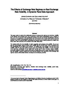
Table 3 shows the result of the Parsimonious error correction model. In this model, while most of the variables are significant at the 1% level. The least statistically significant and statistically insignificant variables were deleted from the model. The log likelihood and Akaike information criterion suggest that the deletion of the variable is useful. Appendix Table 1 shows the result of the overparameterized error correction model. The result of the error correction model shows that nominal effective exchange rate depreciation leads to a depreciation of the real effective exchange rate of Nigeria and this effect holds both in the contemporaneous sense and after a year and the contemporaneous effect is higher than the effect after a year. The result also shows that the price level has negative effect on the real effective exchange rate of Nigeria. This implies that as the price level increases, the real effective exchange rate of Nigeria appreciates. This effect also holds after a year, though it decreases in magnitude. The one period lag value of capital flow has a negative impact on the real effective exchange rate, though the contemporaneous value is insignificant and hence not included in the parsimonious model. This implies that an increase in capital flow to Nigeria in a particular year appreciates the real effective exchange rate in the following year. This implies that the Dutch Disease Syndrome holds in Nigeria with a lag effect. This is not surprising with the over-reliance of the Nigerian economy on petroleum revenue. The openness of Nigeria to international trade has a negative impact on the real effective exchange rate. Thus, commercial policies that encourage trade liberalization in Nigeria depreciate the real effective exchange rate. The result also shows that real GDP has a positive effect on the real effective exchange rate. This is in contrast to the prediction of the Ricardo-Balassa thesis. This result implies that in the short run, real GDP growth comes from the non-tradable goods sector of Nigeria. The ratio of government spending to GDP is insignificant in the model and was not included in the parsimonious ECM Model. This insignificance could be as a result of the fact that the investment variable has both private and government sector components; government expenditure is made up of consumption and investment; and investment is significant in the model. This reflects the fact that over the period 1970 to 2010, government investment was higher than private investment in Nigeria. The terms of trade is also found to be insignificant in the real effective exchange rate model. The insignificance of the terms of trade implies that terms of trade as an external factor has not been an important player in the determination of the real effective exchange rate and hence the determination of the international competitiveness of Nigeria. The significance and negative ECM is an indication that the speed of adjustment has been satisfactory. This further confirms the long run relationship suggested by the Johansen cointegration test. 3.2.4 Diagnostic Tests Various diagnostic tests were carried out in order to determine the robustness of the real effective exchange rate model. Appendix table 2 shows the results of the residual diagnostics tests and the model stability test. The null hypotheses in this case are that there is no serial correlation, the model is homoskedastic and that the errors are normally distributed. The statistical insignificance of the tests is an indication of a validation of the null hypotheses. The results thus show that the residuals of the model are normally distributed, there is no autocorrelation problem, there is no heteroskedasticity problem and there is no autoregressive conditional heteroskedasticity. The cumulative sum of squares (CUSUM) test statistic is updated recursively and plotted against the break points in the data. For stability of the short run, dynamics and the long run parameters of the determinants of real exchange rate, it is important that the CUSUM statistic stay within the 5% critical bound (represented by the straight lines). The CUSUM figure in the appendix shows that the model is stable. 157

www.ccsenet.org/ijef

International Journal of Economics and Finance

Vol. 4, No. 8; 2012

4. Conclusion The real effective exchange rate is a measure of the international competitiveness of an economy and an overvalued real exchange rate increases the price of domestic goods abroad, leading to lower demand for exports. This deteriorates the trade balance. In Nigeria, nominal effective exchange rate increased in the 1970s, 1980s, 1990s and 2000s by either the activity of the government (during the fixed exchange rate regime) or a combination of government intervention and market forces (in the managed floating exchange rate regime which took off in 1986). However, the real effective exchange rate of Nigeria did not follow the trend of the nominal exchange rate. This therefore forms the basis of the investigation of the determinants of the real exchange rate in Nigeria using data covering the period of 1970 to 2008. The variables were tested for unit root as well as cointegration and their short dynamic run relationship using Hendry’s general to specific modelling was estimated. The long run equilibrium real exchange rate was analysed using the Johansen maximum likelihood technique. The result from the error correction model shows that increase in the price level, capital inflow, capital accumulation and trade openness appreciates the real effective exchange rate of Nigeria. This is a major contribution of the this paper because other studies including that by Mungule failed to realise the important influence of the price level on the real exchange rate. Also, an increase in the nominal effective exchange rate and output depreciate the real effective exchange rate. These empirical findings have implications for measures to improve the competitiveness of Nigeria in international trade. First, increases in domestic policies that ameliorate inflation are imperative since increase in domestic price level appreciates the real effective exchange rate. Second, since capital accumulation appreciates the real effective exchange rate, there is need for the creation of enabling environment that encourages investment in the tradable goods sector, rather than the non-tradable goods sector. This can be done by reforming the Nigerian agricultural and industrial sectors to attract investment for the purpose of export and reforming the mining sector for increased investment. Third, given the fact that trade openness appreciates the real effective exchange rate, there is need to integrate Nigeria with other economies in the West African sub-region. Fourth, since real output has a positive impact on the real effective exchange rate, to generate a substantial real exchange rate depreciation, supply side policies that will improve productivity will be useful in Nigeria. This will include human capital development in form of education and health as well the improvement in basic infrastructural facilities like electricity amongst others. References Adewuyi, A. O. (2005). Trade and exchange rate policy reform and export performance of the real sector: The case of Nigeria. Selected Papers for the 2005 Annual conference of the Nigerian Economic society. Bah, I., &Amusa, H. A. (2003). Real exchange rate volatility and foreign trade: Evidence from South Africa’s exports to the United States. The African Finance Journal, 5(2), 1-20. Balassa, B. (1964). The Purchasing Power Parity doctrine: A reappraisal. Journal of Political Economy, 72, 584-96. http://dx.doi.org/10.1086/258965 Box, G. E. P., & G. M. Jenkins. (1970). Time series analysis, forecasting and control, San Francisco: Holden-Day. CBN. (2008). Statistical Bulletin, Golden Jubilee Edition. CBN. (2009). Statistical Bulletin, December Edition. CBN. (2010). Statistical Bulletin Davidson, J., Hendry, D., Sbra, F., & Yeo, S. (1978). Econometric modelling of the aggregate time series relationship between consumers’ expenditure and income in the United Kingdom. Economic Journal, 88(352), 661 –92. Edwards, S. (1989). Real exchange rates, devaluation and adjustment: Exchange rate policy in developing countries. Cambridge: The MIT Press. Edwards, S. (1994). Real and monetary determinants of real exchange rate behaviour: Theory and evidence from developing countries. In: Williamson, J. (ed.). Estimating Equilibrium Exchange Rates. Washington: Institute for International Economics. Engle, R. F., & Granger, C. W. F. (1987).Cointegration and error correction: representation and testing, Ecometrica, 55, 251-76. http://dx.doi.org/10.2307/1913236 Gbosi, A. N. (2002). Financial sector instability and challenges to nigeria’s monetary authorities. Lagos: African Heritage Publication 158

www.ccsenet.org/ijef

International Journal of Economics and Finance

Vol. 4, No. 8; 2012

Granger, C. W., & Newbold, P. (1977). The time series approach to econometric model building, In Obadan, M.I. and Iyoha, M.A. eds. (1996). Macroeconomic analysis: Tools, techniques and applications. NCEMA, Ibadan: Polygraphics Venture Ltd. Hendry, D. F. (1986). Econometric modelling with cointegrated variables: an Overview. Oxford Bulletin of Economic and Statistics, 48(3), 201–12. http://dx.doi.org/10.1111/j.1468-0084.1986.mp48003001.x Hendry, D. F., & Mizon, G. (1978). Serial correlation as a convenient simplification, not a nuisance: A comment on a study of the demand for money of the bank of England. Economic Journal, 88(351), 549-63. http://dx.doi.org/10.2307/2232053 Johansen, S. (1995). Likelihood-based inference in cointegrated vector autoregressive models. Oxford: Oxford University Press. http://dx.doi.org/10.1093/0198774508.001.0001 Mungule, K. O. (1997). The impact of the real exchange rate misalignment on macroeconomic performance in Zambia. MA Thesis, University of Malawi, Zomba, Malawi. Mungule, K. O. (2004). The determinants of the real exchange rate in Zambia. African Economic Research Consortium, Paper 146 Nairobi. Obadan, I. M. (1994). Real exchange rates in Nigeria, 6, 53-70. National Centre for Economic Management and Administration (NCEMA). Ibadan, Nigeria. Obadan, M. I. (2006). Overview of exchange rate management in nigeria from 1986 to date, in the Dynamics of exchange rate in Nigeria. Central Bank of Nigeria Bullion, 30(3), 17-25. Ogun, O. (2004). Real exchange rate behaviour and non-oil export growth in Nigeria. African Journal of Economic Policy, 11(1), June. Oxford dictionary of Economics. Oxford: Oxford University Press Pesaran, H. M., & Pesaran, B. (1997). Working with microfit, 4.0, Oxford University Press. Sargan, J. D. (1964). Wages and prices in the UK: A study in econometric methodology, in P. Hart, G. Mills and J. Whittaker (eds.), Econometric analysis for national planning, London: Butterworths.. Xiaopu, Z. (2002). Equilibrium and misalignment: an assessment of the RMB Exchange rate from 1999, Centre for Research on Economic Development and Policy Reform. Working Paper 127 Appendix 1. Summary of Overparamterized Error Correction Result for Real Effective Exchange Rate Variable

Coefficient

Std. Error

t-Statistic

Prob.

ECM( -1)

-0.101729

0.023410

-4345431

00002

DLTOT

-0.007717

0.017749

-0.434805

0.6686

DLTECHPRO

-0.006500

0.033714

-0.192798

0.8492

DLRGDP

0.133133

0.051155

2602563

0.0126

DLRGDP(-1)

-0.038824

0.099507

-0.390160

0.7008

OLOPEN

-0.073214

0.025428

-2.879235

0.0062

DLOPEN(-1)

-0.004009

0.089342

-0.044873

0.9647

DLNEER

0.939993

0.115227

8.157780

0.0000

DLNEER(-1)

0.861709

0.143721

5.995693

0.0000

DLGSPGDP

0.052982

0.065322

0.811091

0,4274

DLGSPGDP(-1)

-0,012721

0.082357

-0.154464

0,8789

DLCAPFLGDP

-0.020364

0.030082

-0.676957

0.5066

DLCAPFLGDP(-1)

-14.52595

5.933952

-2.447938

0,0204

P

-0960240

0,058651

-16.37203

0.0000

P(-1)

0.004102

0.003942

1,040775

0,3110

C

-0.192428

0.084000

-2.290802

0.0336

R-squared

0.553949

Adjusted R-squared

0.544850

Sum squared resid

1.398024

Log likelihood

8.102643

Durbin-Watson stat

2.426668

Akaike info criterion

0.534992

Schwarz criterion

1.318682

F-statistic

10.38800

Prob (F-statistic)

0 000024

159

www.ccsennet.org/ijef

Inteernational Journaal of Economicss and Finance

Vol. 4, No. 8; 2012

Appendix 2. Results of Model-Residua M al Diagnostic T Tests Breush-Godffrey Serial Correlation LM Test F Statistic

0.576281

Probability

0.569275

Obs* R-squuared

1.630616

Probability

0.442503

White H Heteroskedasticitty test F Statistic

0.808577

Probability

0.696940

Obs* R-squuared

34.49081

Probability

0.444292

ARCH Test F Statistic

0.004997

Probability

0.944061

Obs* R-squuared

0.005290

Probability

0.942020

Jarque Berra

1.293938

Probability

0.1253637

Figure 1. C Cusum Stabilityy Test

160