Real Exchange Rate Volatility, Economic Growth & the Euro

Real Exchange Rate Volatility, Economic Growth and the Euro Thorsten Janus University of Wyoming Daniel Riera-Crichton Bates College Abstract This paper studies the effect of real effective exchange rate (REER) volatility on economic growth as well as the euro’s effect on REER volatility. We first show that, after a plausible endogeneity correction, REER volatility is negatively associated with growth in a 1980~2011 panel of OECD countries. One standard deviation volatility decrease is associated with about two percentage points (0.8 standard deviations) growth increase. Second, we find that euro adoption was associated with a decline of 0.4 standard deviations in long-run REER *volatility before the Great Recession in 2008~09. Moreover, while the Great Recession increased REER volatility by 38-189 percent of the sample mean outside the euro-zone, the REERs of euro adopters were almost completely insulated. We conclude that REER stability may be growth-enhancing in OECD countries and the euro may therefore have played a growth-enhancing role at least before the recent euro-zone debt crisis.

JEL: F31, F32, F33 Keywords: Euro, Great Recession, Economic Integration, Real Exchange Rates

*

Corresponding Author: Thorsten Janus; University of Wyoming, Dept. of Economics & Finance, Dept. 3985, 1000 E. University Ave., Laramie, WY 82071, US; Tel. +1 3077663384, Fax +1 3077665090, email [email protected]. Co-author: Daniel Riera-Crichton; Bates College, Dept. of Economics, Pettengill Hall, Room 273, Lewiston, ME 04240, US; Email: Tel +1 2077866084, email [email protected]. 1

Thorsten Janus and Daniel Riera-Crichton

I. Introduction This paper seeks to address the effect of real effective exchange rate (REER) volatility on economic growth. Although Eichengreen’s (2007) survey concludes that REER stability is likely to be a facilitating condition for growth, it notes that the evidence should be interpreted with caution since few studies control for reverse causality and many rely on a cross-section of countries. Recently Aghion et al. (2009) find that REER volatility is negatively associated with labor productivity growth if financial development is below a threshold. Although their study uses has the advantage of using a panel rather than cross-section of countries, their identification strategy assumes that REER volatility and its interaction with financial development are uncorrelated with future realizations of the error term. In this paper, instead, we study the effect of REER volatility on growth in a panel of OECD countries where we instrument REER volatility with a commodity terms of trade volatility measure. Though it is not entirely clear that REER volatility is the only mechanism linking terms of trade volatility to growth,1 it seems likely to explain most of the transmission. To follow up on the evidence, we further ask how the euro-zone’s common currency adoption has affected the member-countries’ REER volatility.2 Our principal findings can be summarized as follows. First, REER volatility is negatively associated with growth in the OECD sample. One standard deviation decrease in volatility is associated with about two percentage points (or 0.8 standard deviations) growth increase. The estimate contrasts with Aghion el al. (2009), who find a positive effect on labor productivity only in 1

We thank Yao Tang for this observation.

2

Papaioannou and Portes (2008) discuss the potential benefits and costs of the euro in detail. Apart from increasing

REER stability, the euro may increase international trade, investment and liquidity, provide a new global reserve currency, and decrease and stabilize inflation.

Real Exchange Rate Volatility, Economic Growth & the Euro

financially underdeveloped economies. Second, euro adoption was associated with a decline of about 0.4 standard deviations in long-run REER volatility before the onset of the Great Recession in 2008~09. Moreover, while the Great Recession increased volatility by 38-189 percent of the sample mean (or 0.4-2 standard deviations) outside the euro-zone, the REERs of euro adopters were almost completely insulated. On this basis we conclude that the euro may have increased economic growth by stabilizing the real exchange rates of member countries over the sample years. That being said, we should emphasize that our sample ends in 2009, which is just before the recent debt crisis in the euro-zone. In the remainder of the paper, Section II describes our data. Section III studies the effect of REER volatility on economic growth. Section IV reviews the theoretical underpinnings linking euro adoption to REER stability as well as preliminary evidence linking the two empirically. Section V estimates the effect of euro adoption. Section VI concludes the paper.

II. Data We obtain real GDP data in 2005 US dollars from the IMF’s International Financial Statistics (IFS). We use the deflator provided by the IMF to deflate the nominal value of domestic currency GDP and then transform that value into US dollars using the nominal exchange rate provided in the IFS. We also obtain some real GDP data from OECD Source, Economic Intelligence Unit (EIU), DataStream (DS) and the CEIC Data Company Ltd. (CEIC). We then compute GDP per capita with population data from the Penn World Tables. We record total gross capital flows as the sum of the absolute value of all liability increases and decreases plus total asset increases and decreases in the capital and financial balance as reported in the IMF’s Balance of Payments Statistics (BOPS). We additionally obtain current account data from BOPS and domestic consumer price index (CPI) 3

Thorsten Janus and Daniel Riera-Crichton

inflation from IFS, DS, EIU and CEIC. To estimate the effect of REER volatility on growth we use commodity terms-of-trade (CTOT) data from Aizenman et al. (2012). The CTOT index is the ratio of a weighted average price of a country’s main commodity exports to a weighted average price of its main commodity imports. Specifically, the CTOT for country

CTOT jt  ( Pit / MUVt ) i

X ij

/ ( Pit / MUVt ) i

M ij

j

in period t is

, where Pit is a common price index for six commodity

categories (food, fuels, agricultural raw materials, metals, gold, and beverages) in year t ; X ij is country j' s average share of exports of commodity i as a percent of GDP from 1970 to 2009; M ij is the corresponding average share of imports.

The commodity prices are deflated by a

manufacturing unit value index (MUV). Since X ij and M ij are averaged over time, the movements in CTOT jt are invariant to changes in export and import volumes in response to price fluctuations. They, therefore, isolate the impact of commodity prices on the country’s commodity terms of trade. By excluding industrial goods, and concentrating on commodity prices, the CTOT focuses on a highly volatile component of import and export prices. We refer to Aizenman et al. (2012) for more details and data sources. To measure the real effective exchange rate, we use an index which represents a trade-weighted nominal effective exchange rate index adjusted for relative movements in national prices, REER  i [(e / ei )( P / Pi )] i , where e is the nominal exchange rate of the w

subject currency against the US dollar (US dollars per currency unit in index form), ei is the exchange rate of the subject country’s trade partner i against the US dollar (US dollars per currency unit i in index form) and wi is the bilateral trade based weight attached to trade partner i in the index. The weights are calculated based on the sum of bilateral exports and imports. The variable P is the CPI of the subject country and Pi is the CPI of the trade partner. An increase in the REER

Real Exchange Rate Volatility, Economic Growth & the Euro

implies a real appreciation. The data is from the IFS, OECD and JP Morgan. In order to control for the Harrod-Balassa-Samuelson effect, i.e., the hypothesis that productivity tends to grow faster in the tradables than the non-tradables sector and therefore GDP growth may be correlated with REER appreciation (Rogoff 1996),3 we compute relative non-tradables TFP growth as the weighted average TFP growth in non-tradables industries relative to weighted average TFP growth in tradeables industries. The industry TFP growth data is from the OECD Source dataset, where we define agriculture, mining, manufacturing and energy as tradables sectors, and construction, wholesale and retail trade, finance and business sector services as non-tradables sectors. The weights used to aggregate the industries in a sector were calculated using industry value added from UNdata. Lastly, we obtain data for the stock of reserves as the total stock of international reserves minus gold based on IFS, DS and EIU, and we compute trade openness as the sum of merchandise exports and imports divided by twice the value of nominal GDP, all in current U.S. dollars. The data for Imports and Exports was extracted from IFS, DS, EIU and CEIC.

III. Real Exchange Rate Volatility and Output Growth In this section we estimate the effect of REER volatility on growth in a panel of OECD countries. There are several reasons to expect a negative effect. As discussed in Calvo et al. (1996), a volatile REER may encourage foreign-financed spending booms when the exchange rate is high, followed by costly busts due to credit crunches and a rising real value of foreign-currency denominated debt when the exchange rate falls. Martin and Rogers (2000) argue that boom-bust cycles can prevent learning-by-doing and therefore lower the economy’s long-term growth rate. Following Dixit and

3

We thank an anonymous referee for this suggestion.

5

Thorsten Janus and Daniel Riera-Crichton

Pindyck (1994), the uncertainty associated with volatility may induce firms to postpone irreversible investments. Cottani et al. (1990) note that REER volatility may force investors to pay adjustment costs to move across countries or between tradable and non-tradable sectors.4

A. Estimation Strategy In order to identify the empirical growth effect of REER volatility, it is likely to be important to control for reverse causality – e.g., a growth decline might destabilize the REER as foreign capital flees the economy – as well as other sources of potential endogeneity. In order to address the endogeneity concern, we focus on instrumental variables (IV) estimation of the growth rate of real GDP in an annual panel of OECD countries from 1980 to 2011. We measure REER volatility as the standard deviation of the REER over the twelve months of each calendar year and instrument this measure with the standard deviation of the CTOT index described in Section II over the same period. The empirical growth specification is

 g it   0  1 REERVol i (t 1)   2 crisis   3t   4 xi (t 1)  i   it ,

(1)

where g it is the growth rate (change in the natural logarithm) of real GDP in country i in year t , ln Yit  ln Yi (t 1) . On the right hand side, REERVol i (t 1) is the lagged value of REER volatility, 4

As noted the empirical literature remains unsettled. Cottani et al. (1990) find that real exchange rate stability is

associated with increased investment and growth in developing countries. Dollar (1992) and Bosworth et al. (1995) link it to growth and Ghura and Grennes (1993) and Bleaney and Greenaway (2001) link it positively to investment but find no evidence of a growth effect for sub-Saharan Africa. Most recently, Aghion et al. (2009) link REER stability to labor productivity growth in financially underdeveloped economies.

Real Exchange Rate Volatility, Economic Growth & the Euro

Crisis is a dummy for the Great Recession that is equal to one in 2008 and 2009, t is a time trend,  xi (t 1) is a vector of other controls,  i is a country fixed effect and  it is an i.i.d. error term. The

lagged measure of real exchange rate volatility, REERVol i (t 1) , is estimated in the first stage of the IV procedure using the lagged volatility of the country’s commodity terms of trade, CTOTVoli (t 1) , as instrument. Although in principle IV estimation makes it unnecessary to include other growth determinants, we control for the lagged growth rate of TFP in the non-tradables sector relative to the tradables sector, the lagged value of GDP per capita and its square, trade openness, inflation and squared inflation. The first control intends to capture the Harrod-Balassa-Samuelson effect explained in Section II. The other controls capture the stylized facts that middle income economies, more open economies and economies with moderate inflation tend to grow faster. Income per capita, openness and inflation could also be correlated with REER volatility if high-income countries have a larger non-tradables share in GDP, more open economies are more likely to sustain purchasing power parity due to lack of trade barriers, or inflation destabilizes the nominal exchange rate. We refer to Dornbusch (1985), De Gregorio et al. (1994) and Rogoff (1996) for more detailed discussions. Tables 1-2 display the summary statistics and sample countries.

B. Results The estimates in Table 3 are consistent with a negative effect of REER volatility on growth: one standard deviation decrease in REER volatility is associated with 1.7-2.3 percentage points growth increase depending on the specification.5 The first stage estimates show that commodity terms of trade volatility is a good predictor of REER volatility: the Kleibergen-Paap Rk Wald F statistics

5

Including all controls in the same regression yields a very similar estimate of -0.018 (significant at the 10% level). 7

Thorsten Janus and Daniel Riera-Crichton

consistently reject that the model is under-identified and that the true size of the five percent significance test exceeds ten percent due to weak instruments (Stock and Yogo 2005).

IV. The Euro and REER Stability Prior to estimating the euro’s effect on REER stability, we briefly consider the theoretical underpinnings linking the two and some simple preliminary evidence. On the theory side, although it may seem obvious that a common currency implies a fixed exchange rate, this conclusion for the euro would be false for two reasons. First, the euro only fixes exchange rates within the euro-zone. Second, if prices are flexible, the REER can fluctuate despite a common currency. In fact, Berka et al. (2012) take issue with the classical Freidman critique that fixed exchange rates are destabilizing and conclude that (p. 179) “real exchange rates within the euro-zone adhere fairly closely to the efficient outcome.” Berka and Devereux (2013) similarly find that real exchange rates within the euro-zone have adjusted substantially towards purchasing power parity via inflation differentials. In order to link the euro formally to REER volatility, we use that a euro country’s REER can be written

REER   iN1[ei qi )]wi   iM1[ei qi ]wi   iNM 1[ei qi ]wi ,

(2)

where countries 1 to M are other euro countries, countries M+1 to N are non-euro countries,

qi  P / Pi is the domestic currency price level relative to the foreign currency price level of trading

Real Exchange Rate Volatility, Economic Growth & the Euro

partner i , ei is the nominal exchange rate with this trading partner, and wi are bilateral trade weights.6 In logs,

ln( REER )  i 1 wi ln ei qi  i  M 1 wi ln ei qi M

N

(3)

From (3), the variance of the log REER before the euro’s introduction is





2 2 2 2 2  ln( REER )  i 1 wi  ln(e q )  i  M 1 wi  ln(e q )  2 cov i 1 wi ln(ei qi ), i  M 1 wi ln(ei qi ) , M

N

i i

i i

M

N

(4)

where the first term is the variance of the REER against future euro members, the second term is the variance against non-members, and the third term is the covariance of REERs viz-and-viz members and non-members. After the euro-zone is formed, REER variance becomes





2 2 2 2 ~  ln( w 2 ln( w ln(e~i q~i ) , ~  ~ )  2 cov  wi ln qi ,  REER )  i 1 wi  ln q e~ q i  M 1 i i 1 i  M 1 i M

N

i

i ii

M

N

(5)

using that the relative price levels and nominal exchange rates with respect to all trading partners will change to some q~i  qi and e~i  ei , with e~i  1 for the M euro partners. For example, Ireland’s price level relative to both the US and Germany will change and its previous pound-dollar and pound-deutschmark exchange rates are now the euro-dollar exchange rate and unity, respectively. Subtracting (4) from (5) gives the change in REER variance due to the euro: 6

Due to data limitations, in the empirical section we compute the bilateral nominal exchange rates as the ratio of the

two countries’ exchange rates relative to the US dollar.

9

Thorsten Janus and Daniel Riera-Crichton

2  ln( REER ) 

 



 

2 w 2 ln2 q~i  i 1 wi2 ln( ei qi )  i 1 i M

M



2 2 2 w 2 ln( ~ ei q~i )  i  M 1 wi  ln(ei qi ) i  M 1 i N

N



M N M N  2 cov i 1 wi ln q~i , i  M 1 wi ln( e~i q~i )  cov i 1 wi ln(ei qi ), i  M 1 wi ln(ei qi )



 (6)

where the three terms are, respectively, the change in variance against members, the change in variance against non-members, and the change in the covariance term. Equation (6) shows three effects of introducing the euro. The first term is the fall in REER variance relative to euro members due to fixing the nominal exchange rate completely. The second term is a rise in variance if the post-euro REER relative to non-members is more volatile than its pre-euro counterpart. For example, with the loss of autonomous monetary policy, Ireland can nolonger stabilize its nominal exchange rate against its largest trading partner, which is the US. As a result Ireland’s real euro-dollar exchange rate might fluctuate more than its earlier real pound-dollar exchange rate. Its overall REER relative to non-euro members can therefore be more unstable, i.e., the second term in (6) can be positive. The third term can similarly destabilize the REER if, again using the Ireland example, the covariance between the real Pound-Deutschmark and real pounddollar exchange rates before the euro was smaller than the covariance between the relative IrishGerman price level and the real Irish euro-dollar exchange rate. For example, if relative price levels are constant in the short run and the Irish pound used to fall against the dollar when it rose against the deutschmark, then the first covariance term in (6) will be close to zero and the second term will tend to be negative. In this case, prior to the euro Ireland could use the deutschmark to hedge against dollar fluctuations – net exports to Germany might boom when net exports to the US declined – but the euro prevented this hedging.

Real Exchange Rate Volatility, Economic Growth & the Euro

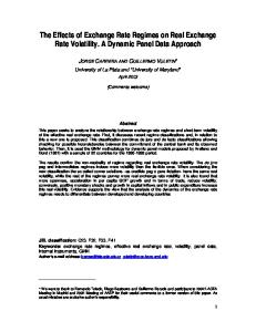
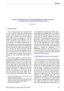
Despite the theoretically ambiguous effect of the euro, Figure 1 suggests that, in practice, the euro has stabilized the member REERs quite significantly. The two curves show the un-weighted country average REER volatility for euro- and non-euro adopters from before to after 1999. While the two country groups show similar REER volatility prior to euro adoption, the euro members had much more stable REERs subsequently. The volatility differential grew sharply leading up to the Great Recession when, as Figure 2 shows, the real depreciations experienced by non-members were larger by an order of magnitude. When we formally decompose the REER variances of individual euro members and the euro-zone overall using Equations (4)-(6) we find the results in Table 4. The trade weights used for the decomposition are average 1970-2006 bilateral trade weights, which we summarize in in Table 5. Table 6 shows that the euro-zone average decline in REER volatility after adoption was mostly (57%) due to decreased volatility against other euro members. However, declining variance against non-members accounted for 17% and less covariance between the REER with members and the REER with non-members accounted for 25% of the total variance decline.

V. Estimation of the Euro’s Effect on REER Volatility In this section we formally estimate the euro’s effect on REER volatility. Because we have sufficient data available and the REER can show high-frequency movements, we estimate a quarterly rather than annual panel. The quarterly volatility of the REER is computed by first calculating the standard deviation between two months prior and two months after the current month. We, then, take the average variance across the three months of every quarter. Formally

REERVol it 





1  s 2,s  2   s 1,s 3   s ,s  4 , 3

(7)

11

Thorsten Janus and Daniel Riera-Crichton

where t and s count, respectively, the number of quarters and the number of months in the dataset.

A. Estimation strategy REER volatility has a strong autoregressive component and least squares dummy variables (LSDV) estimates of dynamic panels suffer from bias due to endogeneity among the independent variables (Nickell 1981). We therefore estimate a random effects model following Hausman and Taylor (1981) and Amemiya & MaCurdy (1986). The resulting Hausman-Taylor estimators are frequently used in dynamic panel estimation and are derived in Greene (2002). Their key advantage is to allow some of the covariates, such as the lagged dependent variable, to be correlated with the unobserved individual-level random effect.7 The estimating equation is the following:

REERVol it   0   1 REERVol i (t 1)   2 Euroi (t 1)   3Crisis (t 1)      4 ( Euroi (t 1)  Crisis (t 1) )   5 xi (t 1)   6 z i   7 t   i   t  vit .

(8)

On the right hand side of (8), REERVol i (t 1) is the first-order autoregressive component, Euro represents a dummy equal to one if the country has adopted the euro and Crisis is a dummy equal to one in Q4: 2008. For robustness we also estimate (8) with two broader crisis definitions, however, including Q4:2008~Q1:2009 and Q4:2008~Q3:2009. As another robustness check we

7

Compared to the Hausman-Taylor approach, a potentially more efficient General Methods of Moments (GMM)

procedure for dynamic panels relies on Arellano and Bond (1991) and Blundell and Bond (1998). However, with 80 quarters per country the length of our times-series exceeds the number of countries. This makes their procedure infeasible in our setting.

Real Exchange Rate Volatility, Economic Growth & the Euro

estimate it separately both in the full OECD sample and in a subsample of European (euro and non-

  euro) economies. The vector xi (t 1) contains lagged time-varying control variables, zi contains  time-invariant controls, t is a time trend,  i is the country-specific random effect,  t is a set of four quarter dummies (to control for seasonality), and vit is the i.i.d. error term. The set of time-

 varying controls in xi (t 1) includes the current account, the change in reserves, total gross capital flows, inflation and its square, and the volatility of the commodity terms of trade. The time-

 invariant controls in zi include regional and non-emerging-OECD country dummies. The use of Hausman-Taylor estimators requires that we specify a set of exogenous and a set of endogenous covariates. We assume that all variables, except the volatility of the commodity terms of trade and euro adoption, are endogenous. However, the results are robust to making all variables endogenous.

B. Results The estimates in Table 7 imply that euro adoption was associated with about 0.23 standard deviations decline in short-run REER volatility before the Great Recession period. As the coefficient on lagged REER volatility is about 0.4, the long run volatility change was about 0.4 standard deviations. However, during the Great Recession the short-run stability gain was larger by an order of magnitude: in the non-euro countries the crisis increased REER volatility by anywhere from 38-189 percent of the OECD sample mean (or 0.4 to 2 standard deviations) depending on the specification. In stark contrast, the crisis had little or no effect on REER volatility in the euro-zone: the sum of the coefficients on Crisis and Crisis*Euro is roughly zero. Since we include country random effects, the positive association between the euro and REER stability does not reflect that euro adopters are inherently more resilient to REER fluctuations. These results lead us to conclude

13

Thorsten Janus and Daniel Riera-Crichton

that the euro has stabilized its’ members real exchange rates significantly and the effect was particularly large during the Great Recession.

VI. Conclusion This paper has studied the effect of real effective exchange rate (REER) volatility on economic growth as well as the euro’s effect on REER volatility. We show that REER volatility is negatively associated with growth in a panel of OECD countries after correcting for potential endogeneity using a commodity terms of trade instrument. One standard deviation volatility decrease is associated with a roughly two percentage point growth increase. We then considered the theoretical underpinnings and some preliminary empirical evidence for the widespread assumption that the euro has stabilized the real exchange rates of member countries. Although the euro can in principle destabilize the REER, in practice we find evidence for a strong stabilizing effect. Euro adoption was associated with a decline of 0.4 standard deviations in long-run REER volatility before the Great Recession in 2008~09. Moreover, while the Great Recession increased REER volatility by 38-189 percent of the sample mean outside the euro-zone, the REERs of euro adopters were almost completely insulated. We conclude that REER stability may be growth-enhancing in OECD countries and the euro may therefore have played a growth-enhancing role at least prior to the onset of the euro-zone debt crisis in late 2009 or early 2010.

Real Exchange Rate Volatility, Economic Growth & the Euro

References Aghion, P., P. Bacchetta, R. Rancière, and K. Rogoff (2009), “Exchange Rate Volatility and Productivity Growth: The Role of Financial Development”, Journal of Monetary Economics, 56(4): 494–513.

Aizenman, Joshua, Sebastian Edwards, and Daniel Riera-Crichton (2012), “Adjustment Patterns to Commodity Terms of Trade Shocks: The Role of Exchange Rate and International Reserves Policies”, Journal of International Money and Finance, 31(8): 1990-2016.

Amemiya, Takeshi and Thomas E MaCurdy (1986), “Instrumental-Variable Estimation of an ErrorComponents Model”, Econometrica, 54(4): 869-80.

Arellano, M., and Bond, S. R. (1991), “Some Tests of Specification for Panel Data: Monte Carlo Evidence and an Application to Employment Equations”, Review of Economic Studies, 58(2): 277– 97.

Berka, M., M. B. Devereux and C. Engel (2012), “Real Exchange Rate Adjustment In and Out of the Eurozone”, American Economic Review Papers and Proceedings, 102(3): 179-85.

Berka, M. and M. B. Devereux (2013), “Trends in European Real Exchange Rates”, Economic Policy, 28(74): 193-242.

15

Thorsten Janus and Daniel Riera-Crichton

Bleaney, M. F and D. Greenaway (2001), “The Impact of Terms of Trade and Real Exchange Rate Volatility on Investment and Growth in Sub-Saharan Africa”, Journal of Development Economics, 65(2): 491-500.

Blundell, R. and S. Bond (1998), “Initial Conditions and Moment Restrictions in Dynamic Panel Data Models”, Journal of Econometrics, 87(1): 115-43.

Bosworth, B., S. Collins and Y. Chen (1995), “Accounting for Differences in Economic Growth”, Brookings Institution Discussion Papers No. 115.

Calvo, G. A, L. Leiderman and C. M Reinhart (1996), “Inflows of Capital to Developing Countries in the 1990s”, Journal of Economic Perspectives, 10(2): 123-39.

Cottani, J.A., Cavallo, D.F., Khan, M.S. (1990), “Real Exchange Rate Behavior and Economic Performance in LDCs”, Economic Development and Cultural Change, 39(1): 61–76.

De Gregorio, J., A. Giovannini, and H. C. Wolf (1994), “International Evidence on Tradables and Nontradables Inflation”, European Economic Review, 38(6): 1225-44.

Dixit, A., Pindyck, R.S. (1994), Investment under Uncertainty. Princeton, New Jersey: Princeton University Press.

Real Exchange Rate Volatility, Economic Growth & the Euro

Dollar, D. (1992), “Outward-oriented Developing Economies Really Do Grow More Rapidly: Evidence from 95 LDCs, 1976-85”, Economic Development and Cultural Change, 40: 523-544.

Dornbusch, R. (1988), “Purchasing Power Parity”, in The New Palgrave Dictionary of Economics (Reprint ed.). London: Palgrave Macmillan.

Eichengreen, Barry (2007), “The Real Exchange Rate and Economic Growth”, Social and Economic Studies, 56(4): 7-20.

Ghura, D., Grennes, T.J. (1993), “The Real Exchange rate and Macroeconomic Performance in Sub-Saharan Africa”, Journal of Development Economics, 42(1): 155–74.

Greene, William H. (2002), Econometric Analysis. New Jersey: Prentice-Hall.

Hausman, J. and W. Taylor. (1981), “Panel Data and Unobservable Individual Effects”, Econometrica, 49(6): 1377– 98.

Martin, Philippe, and Carol Ann Rogers (2000), “Long-term Growth and Short-term Economic Instability”, European Economic Review, 44(2): 359-81.

Nickell, S (1981), “Biases in Dynamic Models with Fixed Effects”, Econometrica, 49(6): 1417-26.

17

Thorsten Janus and Daniel Riera-Crichton

Papaioannou, E. and R. Portes (2008), “Costs and Benefits of Running an International Currency, European Commission”, DG-EC/FIN, Special Report on the European Economy, European Economy Economic Papers No. 348.

Rogoff, K. (1996), “The Purchasing Power Parity Puzzle”, Journal of Economic literature, 34(2): 647-68.

Stock, James H. and Motohiro Yogo (2005), “Testing for Weak Instruments in Linear IV Regression”, in (eds. D. W. K. Andrews and J. H. Stock) Identification and inference for econometric models: Essays in honor of Thomas Rothenberg. Cambridge: Cambridge University Press.

Real Exchange Rate Volatility, Economic Growth & the Euro

Tables and Figures Table 1. Summary Statistics Annual Data used to Estimate the Effect of REER Volatility on Growth Variable

Observations

Mean

Std. Dev.

Min

Max

Economic growth

744

0.028

0.026

-0.048

0.138

REER Volatility

699

2.022

1.384

0.411

10.096

Non-tradable/tradable TFP growth

744

-0.002

0.033

-0.147

0.172

Real GDP/capita

626

25,741

8,850

7,581

59,640

Inflation

744

4.405

5.868

-4.5

84

Trade Openness

528

0.409

0.226

0.079

1.383

Commodity Terms of Trade Volatility

713

0.006

0.006

0.001

0.072

Quarterly Data used to Estimate the Euro’s Effect on REER Volatility REER Volatility

3041

1.323

1.250

0.110

13.847

REER Volatility European Subsample

1192

1.143

1.222

0.114

13.637

Current Account*

2636

-0.004

0.052

-0.75

0.221

Change in Reserves*

2644

0.003

0.028

-0.182

0.305

Total Gross Capital Flows*

2636

0.505

0.842

0.006

9.465

Inflation

3520

0.063

0.074

-0.16

0.954

CTOT Volatility

3520

0.004

0.005

0.000

0.126

CTOT Volatility, European Subsample

1292

0.005

0.007

0.000

0.126

Total Private Gross Capital Flows*

2636

0.445

0.791

0.005

8.613

(Note) *Variables are deflated by nominal GDP

Table 2. Sample Countries Euro-zone

Non-euro Europe

OECD

Austria

Denmark

Australia

Israel

Belgium-Luxembourg

Iceland

Austria

Japan

Finland

Norway

Belgium-Luxembourg

Netherlands

France

Sweden

Canada

New Zealand

Germany

United Kingdom

Denmark

Norway

Greece

Finland

Spain

Ireland

France

Sweden

Italy

Germany

Switzerland

Netherlands

Greece

United Kingdom

Portugal

Iceland

United States

Spain

Ireland

19

Thorsten Janus and Daniel Riera-Crichton

Table 3. IV Estimates for Growth and REER Volatility Sample Second Stage REER Volatility (t-1) Time Trend Crisis 2008-09

OECD GROWH -0.017*** [0.004] -0.000** [0.000] -0.020*** [0.003]

Rel TFP Growth(t-1)

OECD GROWH -0.018*** [0.007] -0.001*** [0.000] -0.018*** [0.004] -0.001*** [0.000]

ln Real GDP (t-1)

OECD GROWH -0.017*** [0.004] -0.001** [0.000] -0.014*** [0.004]

OECD GROWTH -0.012*** [0.004] -0.001*** [0.000] -0.014*** [0.003]

-0.532** [0.260] 0.026** [0.013]

ln Real GDP^2 (t-1) Inflation (t-1)

-0.003*** [0.001] 0.000 [0.000]

Inflation^2 (t-1) Trade Openness (t-1) Under-ID test: Kleibergen-Paap Rk LM Chi-sq P-val Weak ID test: Kleibergen-Paap Rk Wald F statistic Stock-Yogo weak ID test critical values

OECD GROWTH -0.013*** [0.004] -0.001*** [0.000] -0.016*** [0.003]

0.045 [0.030] 17.27 0.000

11.42 0.000

19.78 0.000

17.15 0.000

20.22 0.000

39.06

15.94 Maximal IV Size

24.56

40.99

29.60

10%

16.38

15% 8.96 20% 6.66 25% 5.53 REER REER REER REER REER First Stage Regression Volatility Volatility Volatility Volatility Volatility Commodity ToT Vol* (t) 45.49*** 66.64*** 51.94*** 46.66** 42.51*** [11.189] [17.731] [17.229] [17.893] [10.208] Observations 682 251 462 682 462 Number of countries 22 17 22 22 22 (Note) Robust standard errors in brackets.* significant at 10%; ** significant at 5%; *** significant at 1%. Constant included in all regressions. Annual Data 1980-2011. The controls are included in the first stage regressions, but the results are not reported.

Real Exchange Rate Volatility, Economic Growth & the Euro

Table 4. Variance Decomposition for Real and Nominal Exchange Rates Before the euro’s Introduction Total variance

ln REER Relative To euro-members 7.31E-05

Relative To non-members 0.000219

Covariance

0.000226

ln NEER Relative To euro-members 0.000158

6.59E-05

0.000187

7.07E-05

5.78E-05

5.83E-05

Relative To non-members 0.000113

Covariance

Total variance

-4.52E-06

Austria

0.000181

-0.00015

Belgium

0.000215

9.09E-05

5.85E-05

Finland

0.000464

0.000167

0.000368

-7.1E-05

0.000424

0.00073

0.000906

-0.00121

France

0.000305

0.000137

8.73E-05

7.98E-05

0.00032

0.000208

0.000175

-6.3E-05

Germany

0.000389

7.41E-05

0.000171

0.000144

0.000472

0.000267

0.000406

-0.0002

Greece

0.000996

0.000507

0.000217

0.000272

0.001059

0.000748

0.000139

0.000172

Ireland

0.000587

5.63E-05

0.000466

6.43E-05

0.000474

0.00014

0.000415

-8E-05

Italy

0.000556

0.000245

0.000152

0.000159

0.000557

0.000365

0.000173

1.94E-05

Luxembourg

0.000168

8.89E-05

3.39E-05

4.56E-05

0.000157

8.45E-05

3.67E-05

3.56E-05

Netherlands

0.000223

6.12E-05

9.01E-05

7.14E-05

0.000203

0.000057

9.39E-05

5.16E-05

Portugal

0.000799

0.000276

0.00022

0.000303

0.001407

0.000537

0.000335

0.000535

Spain

0.000801

0.000332

0.000172

0.000297

0.00096

0.000423

0.000202

0.000336

Slovenia Euro-zone average

0.005878

0.00406

0.000633

0.001186

0.044392

0.040077

0.000255

0.004059

0.000771

0.000393

0.000199

0.000179

0.004742

0.004128

0.000262

0.000352

Relative To non-members 2.56E-05

Covariance

After the euro’s Introduction Total variance

ln REER Relative To euro-members 2.77E-06

Relative To non-members 2.91E-05

Covariance

Total variance

2.88E-06

2.56E-05

ln NEER Relative To euro-members 0

Austria

3.48E-05

0

Belgium

0.000033

5.01E-06

3.27E-05

-4.71E-06

3.41E-05

0

3.41E-05

0

Finland

0.000131

1.60E-06

0.000128

1.17E-06

0.000126

0

0.000126

0

France

7.73E-05

1.53E-06

7.09E-05

4.90E-06

6.93E-05

0

6.93E-05

0

Germany

9.83E-05

3.93E-06

9.11E-05

3.27E-06

8.98E-05

0

8.98E-05

0

Greece

0.000181

5.59E-05

7.08E-05

5.44E-05

7.14E-05

2.60E-06

6.42E-05

4.61E-06

Ireland

0.000374

6.72E-06

0.00034

2.79E-05

0.000309

0

0.000309

0

Italy

8.61E-05

2.73E-06

8.33E-05

8.78E-08

8.26E-05

6.93E-09

8.29E-05

-3.57E-07

Luxembourg

4.02E-05

1.96E-05

1.47E-05

5.92E-06

1.41E-05

0

1.41E-05

0

Netherlands

5.53E-05

1.34E-05

3.76E-05

4.33E-06

3.73E-05

0

3.73E-05

0

Portugal

9.74E-05

7.39E-06

7.83E-05

1.16E-05

7.15E-05

0

7.15E-05

0

Spain

0.00014

1.62E-05

9.76E-05

2.58E-05

8.78E-05

0

8.78E-05

0

Slovenia euro-zone average

5.77E-05

6.03E-05

3.67E-06

-6.32E-06

3.97E-06

0

3.97E-06

0

0.00011

1.27E-05

8.69E-05

1.06E-05

8.24E-05

1.95E-07

8.19E-05

3.17E-07

(Note) REER is the real effective exchange rate. NEER is the nominal effective exchange rate.

21

Thorsten Janus and Daniel Riera-Crichton

Table 5. Summary of Trade Weights in the REER Variance Decompositions Non-euro Countries Used in The Variance Decomposition

REER of:

Euro Share

Non-euro Share

Austria

0.65422

0.34578

Belgium

0.80024

0.19976

Finland

0.35079

0.64921

Brazil

Korea

France

0.65568

0.34432

Canada

Mexico

Germany

0.54128

0.45872

Chile

Norway

Greece

0.70119

0.29881

Czech Republic

Poland

Ireland

0.31881

0.68119

China

Russian Federation

Italy

0.64822

0.35178

Denmark

Slovak Republic

Luxembourg

0.84247

0.15753

Estonia

South Africa

Netherlands

0.70740

0.29260

Hungary

Sweden

Portugal

0.59704

0.40296

India

Switzerland

Spain

0.65529

0.34471

Indonesia

Turkey

Slovenia

0.93888

0.06112

Israel

United Kingdom

Euro-zone av.

0.64704

0.35296

Japan

United States

Table 6. Changes in Variance and Covariance from Before to after the Euro

Austria

ln REER  Relative To euro-members -0.00015 -7E-05

0.0000074

-0.0002

ln NEER  Relative To euro-members -0.00016

Belgium

-0.00018

-8.6E-05

-2.6E-05

-7.06E-05

-0.00015

-7.1E-05

-2.4E-05

-5.8E-05

Finland

-0.00033

-0.00016

-0.00024

7.187E-05

-0.0003

-0.00073

-0.00078

0.001212

France

-0.00023

-0.00014

-1.6E-05

-7.49E-05

-0.00025

-0.00021

-0.00011

6.31E-05

Germany

-0.00029

-7E-05

-8E-05

-0.000141

-0.00038

-0.00027

-0.00032

0.000201

Greece

-0.00082

-0.00045

-0.00015

-0.000218

-0.00099

-0.00075

-7.5E-05

-0.00017

Ireland

-0.00021

-5E-05

-0.00013

-3.64E-05

-0.00017

-0.00014

-0.00011

7.98E-05

Italy

-0.00047

-0.00024

-6.9E-05

-0.000159

-0.00047

-0.00036

-9E-05

-2E-05

Luxembourg

-0.00013

-6.9E-05

-1.9E-05

-3.97E-05

-0.00014

-8.5E-05

-2.3E-05

-3.6E-05

Netherlands

-0.00017

-4.8E-05

-5.3E-05

-6.71E-05

-0.00017

-5.7E-05

-5.7E-05

-5.2E-05

Portugal

-0.0007

-0.00027

-0.00014

-0.000291

-0.00134

-0.00054

-0.00026

-0.00053

Spain

-0.00066

-0.00032

-7.5E-05

-0.000271

-0.00087

-0.00042

-0.00011

-0.00034

Slovenia

-0.00582

-0.004

-0.00063

-0.001192

-0.04439

-0.04008

-0.00025

-0.00406

Average

-0.0007

-0.0004

-0.0001

-0.00017

-0.0047

-0.0041

-0.0002

-0.0004

-0.86

-0.97

-0.56

-0.94

-0.98

-1.00

-0.69

-1.00

0.57

0.17

0.25

0.89

0.04

0.08

 Total var.

% change Average % of  variance explained by

 Relative To non-members -8.4E-05

 Covar.

 Total var.

 Relative To non-members -0.00019

 Covar. 0.000152

(Note) REER is the real effective exchange rate. NEER is the nominal effective exchange rate. Variance is the average 12 month variance with one observation per year. The basis for decomposition is the following formulas:

REER   iN1[ei ( P / Pi )]wi   iM1[ei ( P / Pi )]wi   iNM 1[ei ( P / Pi )]wi NEER   iN1[ei ( P / Pi )]wi   iM1[ei ]wi   iNM 1[ei ]wi , where countries 1 to M are euro countries and M+1 to N are non-euro countries. The covariances are 2* Covariance(X,Y).

wi

are bilateral trade weights.

Real Exchange Rate Volatility, Economic Growth & the Euro

Table 7. The Euro and REER Volatility Euro+ Euro+ Euro+ Non-euro OECD Non-euro OECD Non-euro Europe Europe Europe Crisis Crisis Crisis Crisis Crisis Crisis 08q4 08q4 08q4-09q1 08q4-09q1 08q4-09q3 08q4-09q3 REER Vol REER Vol REER Vol REER Vol REER Vol REER Vol 0.4163*** 0.4091*** 0.4264*** 0.4123*** 0.4321*** 0.4146*** REER Volatility (t-1) [0.0187] [0.0216] [0.0192] [0.0222] [0.0193] [0.0222] Euro Dummy -0.3202*** -0.2668*** -0.3131*** -0.2632*** -0.3272*** -0.2733*** [0.0683] [0.0606] [0.0693] [0.0618] [0.0691] [0.0616] Crisis (t-1) 2.0889*** 2.6679*** 0.5311*** 0.6762*** 0.3519 0.6948*** [0.2813] [0.3389] [0.1849] [0.2230] [0.2227] [0.2665] Crisis * Euro (t-1) -1.9260*** -2.5066*** -0.7174*** -0.8573*** -0.5305* -0.8601*** [0.3782] [0.3957] [0.2417] [0.2529] [0.2825] [0.2970] Current Account (t-1) -0.9529** -0.9141** -0.9976** -0.9170** -1.0577** -0.8987** [0.4643] [0.3913] [0.4733] [0.3998] [0.4736] [0.4002] Δ International Reserves (t-1) -0.7544 -1.3875** -0.6455 -1.0872* -0.6262 -1.1268** [0.6230] [0.5575] [0.6287] [0.5644] [0.6297] [0.5670] Total Gross Flows (t-1) 0.0790** 0.1231*** 0.0719** 0.1209*** 0.0708* 0.1210*** [0.0361] [0.0313] [0.0365] [0.0317] [0.0366] [0.0318] Inflation (t-1) 1.3947 0.454 2.212 1.1114 2.3808* 1.2207 [1.3900] [1.3160] [1.3964] [1.3287] [1.3999] [1.3303] Inflation^2 (t-1) -2.0416 0.0949 -4.8514 -2.0591 -5.1956 -2.221 [5.4876] [4.9329] [5.5175] [4.9844] [5.5346] [4.9942] Commodity ToT Volatility (t-1) 14.0485*** 13.6326*** 16.7447*** 16.5377*** 18.0212*** 16.3753*** [4.1842] [3.7610] [4.3943] [3.9437] [4.4782] [4.0162] 2440 1774 2440 1774 2440 1774 Observations 22 16 22 16 22 16 Number of countries (Note) Standard errors in brackets. * Significant at 10%; ** significant at 5%; *** significant at 1%. Constant, time OECD

trend and quarter dummies are included in all regressions.

23

Thorsten Janus and Daniel Riera-Crichton

Figure 1. REER Volatility 8 REER Volatility Euro Countries

7 REER Volatility Non Euro European Countries

6 5 4 3 2 1

M1 2009

M1 2008

M1 2007

M1 2006

M1 2005

M1 2004

M1 2003

M1 2002

M1 2001

M1 2000

M1 1999

M1 1998

M1 1997

M1 1996

M1 1995

M1 1994

M1 1993

M1 1992

M1 1991

M1 1990

M1 1989

M1 1988

M1 1987

M1 1986

M1 1985

0

(Note) The two curves show average REER volatility for euro- and non-euro adopters before as well as after euro adoption in 1999.

Figure 2. Real Effective Exchange Rates 0.03 0.02

Q4 2009

Q3 2009

Q2 2009

Q1 2009

Q4 2008

Q3 2008

Q2 2008

Q1 2008

Q4 2007

Q3 2007

Q2 2007

Q1 2007

Q4 2006

Q3 2006

Q2 2006

Q1 2006

Q4 2005

Q3 2005

Q2 2005

Q1 2005

Q4 2004

Q3 2004

Q2 2004

Q1 2004

Q4 2003

Q3 2003

-0.01

Q2 2003

0

Q1 2003

0.01

-0.02 All

-0.03

Euro Non Euro OECD

-0.04

BRICK

-0.05

(Note) We include the emerging markets of Brazil, Russia, India, China and South Korea (BRICK) for comparison.)