© 1978 by Mrs Raymond G. Bressler and Richard A. King.
chapter
/ 3
ECONOMIC INTERDEPENDENCE AND INTERREGIONAL TRADE
The previous chapters have described in some detail the evolution of the American economy from the largely subsistence agriculture of the early colonial period to the industrialized society of today. This evolution has been based on the growth of economic specialization —the division of labor. During the early days of this country each family did almost everything for itself (growing crops and livestock, storing grain and curing meat, grinding meal and flour, making butter and cheese, spinning yarn, weaving cloth, and making clothes) while selling or exchanging a few products in order to obtain the commodities that were difficult or impossible to produce at home. Today very few families are self-sufficient in this way. Instead, they have become highly specialized cogs in a complex economic machine. The commercial farmer may produce a single crop or a relatively small number of products, and little, if any, of this production will be consumed directly by the farm household. The industrial worker may be even more specialized, perhaps performing a single operation in an assembly line or factory. Each obtains a flow of money income by means of these activities — income from the sale of products for the farmer and businessman and income from wages for the laborer. And each, in turn, uses his income to purchase goods and services made available through our exchange or 47
© 1978 by Mrs Raymond G. Bressler and Richard A. King. 48
PROLOGUE
market economy. In this chapter, we provide insights concerning these interrelated flows and their relevance to the development of a modern economic system.
3.1
INTERDEPENDENT ECONOMIC ACTIVITIES
Agriculture has been pictured as a broad aggregate within the economic system in which originates the flow of farm commodities within agriculture and, from agriculture, to other major industries or sectors. Also, there exists a reverse flow of goods and services (including labor) from these other sectors back to agriculture. Similar circular flows of inputs and outputs could be described for every sector and all of them interconnected to represent the flows of goods and services throughout the entire economic system. Needless to say, this representation would be very complex if it showed the interrelations among the major industrial sectors in the system and would be indescribably involved if it attempted to trace out the flows among millions of individuals as producers and consumers. An appreciation of these flows may be gained by thinking for a moment about the systems required to produce and to place thousands of commodities on the shelves of a modern supermarket. Such detailed descriptions are far beyond the scope of this book, but the essential nature of the economic mechanism can be illustrated by simpler aggregations. Consider first a model of the total economy based on three large aggregates: (1) the production aggregate including farming, hunting and fishing, mining, construction, processing, and manufacturing activities; (2) the service aggregate including transportation, trade, communications, and all other business, personal, and professional service activities; and (3) the final demand aggregate including households, government, and foreign countries (this aggregate also represents the basic inputs of resources of land, labor, and capital owned by households, government services paid for by taxes, and the import of goods and services from foreign countries). This highly aggregated model may be represented graphically by two circular flows: one showing the "sale" or input of goods and services from each aggregate to the succeeding aggregate and the other showing the "purchase" of goods and services by each aggregate from the preceding aggregate (Figure 3.1). To make our discussion more concrete, we use data from a study of the United States economy in the year 1947. The production aggregate sold $38 billion of commodities to the service aggregate and, in turn, purchased $41 billion of services. Also, production sold $120 billion to the final demand sector and bought $117 billion. Notice
© 1978 by Mrs Raymond G. Bressler and Richard A. King. ECONOMIC INTERDEPENDENCE AND INTERREGIONAL TRADE
49
FIGURE 3.1 The flows of goods and services among three major sectors of the United States economy. All data are for the year 1947 and are given in billions of dollars. The figures in parentheses represent transfers within indicated sector. This diagram is based on Table 3.1.
that the sales and purchases between any two aggregates need not balance but that there is a balance between any single aggregate and the rest of the economy. Thus, the production aggregate had an unfavorable balance of purchases over sales with the service aggregate amounting to $3 billion and a compensating favorable balance of $3 billion with the final demand aggregate. These interactions can be shown by an input-output table or matrix (Table 3.1). Here each aggregate appears as a "producing" or selling sector in the left-hand stub of the table and also as a "consuming" or purchasing sector at the top of the table. Each column shows the inputs from other industries to the particular purchasing industry; that is, (1) the production aggregate purchased $41 billion from (2) distribution and services and $117 billion from (3) the final demand or autonomous sector. Also, the production sector had internal transfers amounting to $119 billion and, hence, a total gross input of $277 billion. In a similar way, each row in such a table shows the distribution of the output of the indicated sector, or aggregate to all other sectors. The total gross output of the production aggregate-equal to the total gross input for the aggregatewas distributed as follows: (1) $119 billion transferred back into the production aggregate, (2) $38 billion sold to the service aggregate, and (3) $ 120 billion to the final demand aggregate. Input-output tables permit the representation of far more detailed industry interactions than would be possible with graphic means. Tables
© 1978 by Mrs Raymond G. Bressler and Richard A. King. 50
PROLOGUE
TABLE 3.1 Summary of the Flows of Goods and Services Among Three Major Sectors of the United States Economy, 1947 Purchasing Sectors (Billion Dollars) Producing Sectors and Total
Production and manufacturing Distribution and service Autonomous sector payments Total gross inputs Total net inputs
Production, DistriManufac- bution Service' turing3
Final Demand0
Total Gross Outputd
Total Net Output5
119
38
120
277
158
41
40
109
190
150
117 277 158
112 190 150
72 301 229
301 768
229 537
Source. Compiled from Wassily W. Leontief, "Input-Output Economics," Scientific American, Vol. 185, no. 4, October 1951, pp. 15-21, and from the aggregates based on Leontief by Ronald L. Mighell, American Agriculture, Its Structure and Place in the Economy (New York: John Wiley and Sons, 1955), p. 182. "Agriculture, mining, fishing and hunting, construction, and all other manufacturing industries. Transportation, trade, communication, public utilities, finance, insurance, real estate, and all business, personal, and professional service industries. c Households, government, foreign countries, inventory changes, and gross private capital formation. d The sum of outputs (or inputs) for the three major sectors. "The gross output (or input) less transfers within each major sector. have been constructed dividing the United States economy into 500 sectors (an interindustry matrix with 500 rows and 500 columns). Although this huge table is still a tremendous simplification of the true economy, it nevertheless does give in considerable detail the interrelations and interdependencies in the economic system. An "11-by-l 1" condensation of such a matrix is given in Table 3.2. Notice that Table 3.1 is simply a further condensation of this 11-industry table. The production aggregate in Table 3.1 represents the first three sectors of Table 3.2; the service aggregate combines sectors 4 through 7 in Table 3.2; and the final aggregate in Table 3.1 is the sum of sectors 8
© 1978 by Mrs Raymond G. Bressler and Richard A. King.
—;
Vi
—
—
VO >0 • * ") V0 [-; CN ~ CN ^ r OS cn cn 00 t Is VO CN VO CN e'-
oo
en VO —* •—
so r-
S s I-
•
*
•
*
SO K-s 00 •*
• *
os
r-
OS
oo vd
•a B
o
BO E
o vo
d
• —< v o I O n d *
CN
c o
d —
CN
cn CN «o Os ~ —' CN
— oo
vq —• d 'n
OS CN
•* —
t ^ Tf »
—
CN
s:
OS
vq os
d
CN
t
to
m
i n oo r^
•a E 00 E
T3 B
CN vo
T3
so
p
3
a
c VD CN
"
^ t r-- C-- oo CN cn d CN d d os' Tt
•a c oo c
vi
o Vi aj o E 0> — ca ca .*u E
,-
•
CD
Vi
E T3 ca E > o ca ca B ca Dcn r- E
vi
3
C
.5
"S = « "2 S £r o g 0 oo O B
E -r;
E
XI CL> vi
73 ^
g £ > =
L£
> o ° ° " £s.OI
r-~ oo os o
—•
T3 o
2
ca E O Di
io" in w os —
Jj
§
a
a
o a.
E
1 ^ 2 °3 •a o E ni
. la E o 'w O 3
o
.3 a ca B U O cu ca •3 •a ca
3 •a E
o
^) o O on
E ca
E b ~ca -o c/s Q u
j;
oj;
51
-
3 -a o £
© 1978 by Mrs Raymond G. Bressler and Richard A. King. 52
PROLOGUE
through 11 in Table 3.2. It should be pointed out that total gross inputs and total gross outputs in Table 3.2 are equal for each of the first 7 sectors but are only equal in the aggregate for the last 4 sectors. Exports need not equal imports nor government expenditures equal tax receipts, for example, but in the aggregate these final sectors and the entire matrix must balance. Before leaving these interindustry matrices, we must emphasize that they provide more than a convenient description of the national economy. These tables may be used to trace out the approximate impact of changes in certain sectors on the entire system. For example, suppose that the required output of agriculture and fisheries (row 1) increased by 10 percent. Barring changes in technology and in relative prices, this would mean a 10 percent increase in the inputs to agriculture and fisheries, that is, all entries in column 1 would be increased by approximately 10 percent. Corresponding to these changes, there would be upward adjustments in the total output of all other sectors which, in turn, would require input adjustments. In this way, the direct and indirect effects of the increase in agricultural and fisheries output can be traced through the whole economic system. For this reason, detailed input-output tables have been useful planning tools for diverse activities such as war strategy (to determine where strategic bombing .will have the major disruptive effect on an economy) and the industrialization of underdeveloped countries (to check the internal consistency of proposed developments). Even the highly aggregated 11 -industry model suggests the complex and interdependent nature of the economy: changes in any small sector spread out like ripples on a pond and have direct or indirect effects on all parts of the economic system.
3.2 INTERDEPENDENCES WITHIN THE AGRICULTURAL SECTOR Input-output analysis is also useful as a device for studying the relationships within as well as between sectors. Food, textile, and tobacco manufacturers are the primary receivers of farm products, but agriculture also sells directly to many other industries, to households, and to itself. Internal transfers in the form of feed, seed, and livestock amounted to more than $10 billion in 1947, or about 25 percent of the total gross output of the farming sector (Table 3.3). Three-quarters of this internal transfer was from the food and feed grain enterprises (row 4): $3,841 million went to the meat animal enterprise; $1,279 million to poultry and eggs; $1,755 million to dairy products; $817 million back to grain enterprises as seed and as feed for workstock; and the balance of $234
© 1978 by Mrs Raymond G. Bressler and Richard A. King.
in
c o
ooooovocn S o u
£ n "^
cn © cn CN TJ&\ c^t ~* as
vo «H ^
vo
OSOCNVO csi r - cn
H U 00 r-« cn
ca oo
T3 CJ
o
u
3 « "S P ^ E
ca
XI
u B O C3
Ir s B ja O 'C X) ca u E q ca ca _£ u ca 60 CO — o £o < O t60
B 1
•5 *
Is
a o
00
la •= E -o - o £ o ca o U, tt,
60
O o 'oB o
T3 XI 3 E o •a ca oo o u
CO
ca . 5
Q 3
a.
CM
CD
•