A new method for Principal Component Analysis of high-dimensional data using Compressive Sensing Sebastian Klenk [email protected] Gunther Heidemann [email protected]

Intelligent Systems Department Stuttgart University Universit¨atsstrasse 38 70569 Stuttgart, Germany April 8, 2010

Abstract Principal Component Analysis of high dimensional data often runs into time and memory limitations. This is especially the case if the dimension and the number of data set elements is of about the same size. We propose a new method to calculate Principal Components based on Compressive Sensing. Compressive Sensing can be interpreted as a new method for data compression with a number of positive features for application in Statistics. We will demonstrate its usability for Principal Component Analysis by mentioning relevant results from literature and show our results for real world functional data.

1

Introduction

Principle Component Analysis (PCA) is one of the most commonly used methodologies in the Statistics and Data-Mining community. It serves as a general purpose tool with applications ranging from information extraction over dimension reduction to data visualization. Because of its applicability, the range of data subject to PCA is also increasing. From sociological and small scale medical data with dimensions in the tens, data sets and dimensions have grown to sizes beyond tens of thousands and even millions

1

for biomedical or multimedia data. This increase in size pushes current algorithms to their limits. In this paper we will present a new methodology for Principal Component Analysis based on Compressive Sensing. We will show the applicability of this technique by presenting the relevant theory in the light of PCA and by applying it to real world data (in our case heart sound data). As dimension increases Principal Component Analysis has several problems to cope with. Besides pure computational aspects memory requirements often make classic approaches infeasible. Heidemann calculated Principal Components (PCs) of natural images of a large image database where the Covariance Matrix alone would have required an estimate of 2.5 GB of memory (for 128×128 pixel color images) Heidemann [May 2006]. For video data, this could even be surpassed by factor 1000 and more. In Section 2.1 PCA will be introduced and discussed more closely. There problems with the two most commonly used methods for calculating PCs will be presented and related to compression. Compressive Sensing (CS) is currently, to our best knowledge, not discussed as a method for compression but for reconstructing sparse signals about which only very little information – only that of very few random measurements – is given. We want to present a different view. One which shows CS in the light of compression. In Section 2.2 we therefor will introduce CS in more detail and present some established theory related to the use of Compressive Sensing as a means for compression of functional data (data that inhibits a certain degree of smooth change in value) and for the purpose of PCA. The literature about Principle Component Analysis and related topics is vast. PCA is a commonly used methodology and even whole books have been written on it Jolliffe [1986]. We will therefor concentrate on selected publications to present the current state of the art in Principal Component Analysis. Probably the first contact points when starting to read about PCA are textbooks on Statistics, Machine Learning or Pattern Recognition Ripley [2007], Hastie et al. [2002], Bishop [2006, 2000]. In these books several methods for obtaining Principal Components, like the Eigenvalues/ -vectors of the Covariance Matrix or the Singular Value Decomposition, are discussed. Beyond that other methods for the estimation of PCs have been developed. Tipping and Bishop Tipping and Bishop [1997] implemented PCA in a density-estimation framework and developed a EM-based algorithm. Bishop Bishop [2006] describes in his book PCA for high-dimensional data. He notes that even if the dimension d of the data is larger than the 2

number n of elements in the data set, one can only calculate as many PCs as there are data set elements. Further he describes a method to calculate the PCs with a matrix of the dimension squared the number of data-points as opposed to squared the number of dimensions. For n ≪ d, the number of elements is much smaller than the number of dimensions. This leads to better performance and allows the computation of PCs which where before not computable. In situations – which, for high dimensions, are rather rare – where n ≈ d, size of the data set and the number of dimensions are approximately close, this method doesn’t help much. In such a situation a method is needed that actually reduces the size of the data to a degree which makes PCA feasible for approaches described in the literature mentioned above.

2

Theory

The purpose of this section is to give a short overview of methods and ideas behind Principal Component Analysis and Compressive Sensing. Especially for the later, theoretical results from literature will be presented. This is done with the intention to show the reader what motivated the use of CS for effective compression and also to state that this use is justified by sound theory. In the preceding section the ideas and results below will be applied to real word data.

2.1

Principle Component Analysis

For a data set X = {xi |i = 1...n} ⊂ IRp and a corresponding matrix M ∈ IRn×p whose rows are the elements of X one can find a representation zk ∈ IRm for xk which consists of uncorrelated components and maximizes the variance of the new set Z = {zk }. When looking for this new representation one hopes to find one with dimension m ≪ p, which broadly speaking means that less information is needed to describe the same phenomenom. In mathematical terms this is being achieved by calculating the Eigenvalues λk and -vectors ak of the Covariance Matrix. They represent the Principal Components of the data set. The above mentioned new representation can then be obtained by projecting the data X onto a subspace spanned by the Eigenvectors ak of the Covariance Matrix. MZ = M A For p-dimensional data the number of Eigenvectors is equal to the number of dimensions. To achieve the hoped for reduction in dimension, the subspace 3

one projects to must be smaller in dimension then the original space. This means that A must contain less than p Eigenvectors. Which Eigenvector to choose for the projection plane depends on their Eigenvalue. In terms of variance the Eigenvalue corresponding to a Eigenvector gives a measure for its degree of variation preservation: λk = var(aTk x). Besides that the sum of the diagonal elements (the variance of the columns of the data) of the Covariance Matrix is equal to the sum of the Eigenvalues. To calculate the PCs there are several ways described in literature. The direct approach is to calculate the sample Covariance Matrix 1 T M M n and then the Eigenvalues, -vectors pairs thereof. After that, order them by the size of the eigenvalues and take the first m Eigenvectors as Principal Components. For this approach, if one would calculate all p PCs, it would require O(p3 ) operations. A method with less computational effort would be to calculate only the first m Eigenvectors which would involve O(mp2 ) calculations Golub and Van Loan [1989], Bishop [2006]. Another and more commonly used approach involves the Singular Value Decomposition (SVD). There a Matrix M is split into three parts which, when multiplied, result in the matrix itself. S=

M = U ΣV T U is a n × p, Σ a diagonal- and V a orthogonal p × p matrix. The connection between SVD and PCA is based on the fact that the diagonal of Σ contains the square root of the Eigenvalues of S and the columns of V form the Eigenvectors. V (M T M )V T = diag(λ1 , ...λp )

with

λk = σk2

By using the SVD it is rather easy to compute the PCs just by decomposing the data matrix. As opposed to the classic approach no further calculations of the Covariance or Correlation Matrices are needed. The Singular Value Decomposition requires in its batch-mode (taking the whole data matrix at once) O(n2 p + np2 + p3 ) computations Golub and Van Loan [1989]. There are incremental methods for calculating the SVD Brand [2002] which require O(npr 2 ) time with r = min(n, p) and O(np) space. This is much faster then the above mentioned cubic complexity but still the bottle neck is the space requirement for large data with many elements (n ≈ p). 4

2.2

Compressive Sensing

The space requirements of PCA for large data sets calls for some form of data compression. For natural data, i.e. data coming from natural sources like speech, heart sounds, images or financial data a high degree of compression is usually possible and regularly achieved. This is due to the fact that, once the data is transformed to a different representation only a small number of data elements is non-zero. This sparse representation is exploited by just saving the relevant data. For PCA methods or related methods this is either error prone or inefficient because the non-zero elements are not alway in the same position. For different data different transformation coefficients are relevant. So either one saves all relevant coefficients – which would mean that, in the worst case, there is no compression at all – or one chooses in advance which coefficients to keep, which to ignore and thereby risks to loose important information. Compressive Sensing also takes advantage of spare representations of data but as opposed to the above mentioned approach to compression, CS exploits sparse elements independent of their position through a kind of random overall measurements. As a result one gets a set of measurements that incorporates all the relevant information about the data. The main theorem of Compressive Sensing states that for data xk ∈ X ⊂ IRp with a number of non-zero elements being equal to S, the program (P 1)

min kxk1 x

subject to

UΩ x = UΩ xk

where U is an orthogonal matrix and Ω a random subset of the row indices, recovers xk with high probability Candes [June 2007]. Ω and S are connected to X through the following inequation. |Ω| ≥ Const · µ2 (U ) · S · log p

(1)

with µ(U ) = max |Uij |. i,j

The three formulas above state that even if the number of elements which Ω contains is small, compared to the dimension of xk , we are still able to recover xk . This is exactly what compression does – take a signal and reduce as much information as possible without sacrificing reconstructability. In the language of CS the matrix U is responsible for the measurements of the signal xk and is called measurement ensemble. In the literature measurements mj = (mij ) are usually taken in a non deterministic way. This 5

means an inner product of the data xk with a random vector φj is calculated and forms the measurement. mjk = hφj , xk i

with

φij ∼ N (0, 1)

(2)

The measurement ensembles U = Φ is then a random matrix. Cand`es, Romberg and Tao showed in Candes et al. [Feb. 2006] the above mentioned result for the Fourier Matrix U = F 1 Fjk = √ e−i2πkj/n n and in Candes [June 2007] Cand`es generalized this to orthogonal matrices U with U T U = nI where the n is due to more easier handling together with the Fourier Matrix. A special feature in Compressive Sensing is that even though the selection of measurements is non adaptive the recovery still is optimal. Here non adaptiveness means that the knowledge gained during previous measurements is not used when selecting further measuring points nor is any prior knowledge about the function used at all. Cand`es and Tao Cands and Tao [2006] showed that knowing the results of O(K log p) CS measurements is as good as the knowledge about the K largest coefficients of a signal representation. This is what makes CS so interesting as a methodology for compression in the area of Statistics and Pattern Recognition. You neither have to know the largest elements of a data representation nor do you have to know their position. Only a small number of random measurements is sufficient to get a almost exact representation of the data. The Program (P 1) describes a optimization problem that is also known as Basis Pursuit. The basic idea thereby is to find a vector x that is as sparse as possible and still satisfies the constraints given by UΩ . As a measure of sparseness the ℓ0 quasi-norm is theoretically the method of choice. kxk0 = |{i|xi 6= 0}|

and

kxk1 =

n X i=1

|xi |

Practically it is computational not feasible for larger dimensions. In such situations, the ℓ1 norm, as done above, will be preferred. P 1 can than be cast into a Linear Programming optimization problem, even though the absolute value in the minimization functional is a non linear term, by splitting the variables in a positive and negative part Shanno and Weil [1971]. 6

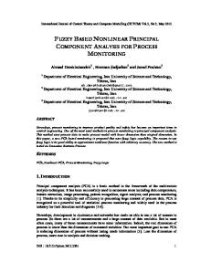
0.20 0.15 Eigenvalues

0.10 0.05 0.00 0

10

20

30

40

Figure 1: Resulting Eigenvalues (light) compared to the original Eigenvalues (dark)

2.3

Adaptive Smoothing

Until now we only talked about sparse representations of functions and what the effects are of having such a representation, but not so much about how to obtain such an representation. This will be the main focus of this section. For CS to be applicable you need a sparse representation of the data. This means that most of the coefficients are zero or can be safely set to zero. In case of the Fourier transformed representation, the Fourier Coefficients decay faster for smooth functions Grafakos [2004]. A sparse Wavelet representation, depending on the wavelet, can also be interpreted as an indication for a smooth function Daubechies [1992]. Therefor when talking about data we think of what Ramsay and Silverman Ramsay and Silverman [2002] consider functional data – a series of measurements that inhibit a smooth variation in its values. Most data that is obtained through measurements is not as smooth as it should be and it is usually corrupted with random noise and artefacts. For many transformed representations this means that the number of non zero elements decreases as the signal to noise ratio increases. Because random noise is the exact opposite of a smooth function, a signal which has been altered with it also ceases to be smooth. To overcome this obstacle we are applying smoothing methods to the data – which can be done in the 7

transformation domain – to obtain a sparse representation. The smoothing methodology we use is based on the SureShrink Algorithm described by Donoho and Johnstone Donoho and Johnstone [1995]. They proposed a soft-thresholding approach to shrink wavelet coefficients with an risk estimate given by the Stein Unbiased Estimate of Risk (Sure). Each element xi of the data is set to zero or decimated by tS depending on its absolute value. To calculate the threshold tS Donoho and Johnstone give the following formula. tS = arg min SU RE(x, t) t≥0

with

p X (|xi | ∧ t)2 SU RE(x, t) = p − 2 · {i : |xi | ≤ t} + i=1

In the same article they also mention a way how this could be used with Fourier Coefficients – instead of the proposed wavelets – where the coefficients are grouped into sections and then shrinked on a section basis.

3

Results

In the previous Sections we have presented our basic idea for solving the problem of PCA in high dimensions as well as some theoretic foundations. The current section will present results obtained by using those ideas for high-dimensional heart sound data. The main emphasis in this section is to demonstrate the idea of a CS preprocessing for an easier high dimensional PCA and to validate the obtained results. For the sake of fast implementation the programming was done with the Statistics programming language R which not always gives good performance. Therefor and because we haven’t done any speed or memory optimizations yet the results presented here focus on error-measures and not on computational speed.

3.1

Procedure

To validate our computational results, we calculated the CS-PCA (Compressive Sensing PCA) and the classic PCA simultaneously and compared the results. The procedure (or algorithm) which we followed to calculate the PCs in a Compressive Sensing Setting is presented in pseudo code as

8

4 2 0 −2 −4

1000

2000

3000

4000

5000

0

200

400

600

800

1000

−2

−1

0

1

2

0

Figure 2: Resulting Eigenvectors (light) compared to the original Eigenvectors (dark)

9

Algorithm 11 . In a first step the transform matrix and the measurement ensemble (in the algorithm called compression matrix) are generated given the data and the type of measurement ensemble. The, for the compression matrix, relevant information is the type of measurement ensemble – how do we want to measure – and the dimension of the data – how many measurements should we take. Together they form the compression matrix by describing how many columns to select (randomly) and what these should look like (from what type of matrix to select them from). In our case the transfer matrix is a Fourier matrix and the compression matrix is a random matrix. The number of dimensions the compression matrix has must be cho√ √ sen in accordance with (1). We did some tests with p log p and c p log p as well as K log p where K is the maximum number of non zero components in the sparse representation. The best results we achieved with the first one of them. All in all the first three rows of the algorithm transform the data into its frequency representation. After that the data will be preprocessed, basically the smoothing method described in Section 2.3 will be applied to the transformed data to obtain a sparse a representation DT s in the frequency domain. The then following step is just a matrix multiplication of the measurement ensemble C with the sparse representation of the transform data matrix. Basically this is just a series of inner products as described in (2). the Once the compressed matrix is calculated, the usual PCA can be calculated. This can be done, either by Eigendecomposition (of the Covariance Matrix) or by Singular Value Decomposition. The calculated Eigenvalues, which correspond to the actual Eigenvalues (see figure 1), give a clue about how many Eigenvectors need to be reconstructed. This is being done, as described in Section 2.2, with the help of the linear programming optimization technique.

3.2

Numerical Examples

We calculated the PCs for a collection of heart sound as representatives of functional data. We have n = 43 heart sounds with a dimension ranging between p = 5000 and p = 20000. For comparability and to cover all data samples we calculated PCs for different values of p (from 500 to 5000) where data with high dimension is simply cut to the right size. Although we haven’t worked on time optimization the algorithm presented above gives compara1 To keep the size of the algorithm in a readable range we described the calculations as matrix calculations, this can be changed easily to keep memory consumption at a minimum.

10

Algorithm 1 CS-PCA (D,Ctype ) T ←getTransferMatrix() C ←getCompressionMatrix(D, Ctype) DT ← D · T DT s ←smoothMatrix(DT ) DC ← DT s · C E ←getPCA(Dc ) P for all λi ∈ E such that λi large enough do i

ei ←reconstruct(eλi ) end for return {ei } ble results, concerning speed, for dimensions below 1000. It is even faster than standard PCA (based on Eigenvalue decomposition of the Covariance Matrix) for higher dimension. For an impartial comparison although both methodologies need to be compared in an equivalent fashion, i.e. state of the art PCA algorithms against optimized CS algorithms. In case of numerical correctness of the calculations the results are comparable. We used correct PCA implementations and calculated PCs which are than compared to the results given by the CS-PCA algorithm. The error measures given by the mean squared error E2 for normalized data are given in table 3.1 below. The values in the table are scaled (by factor 105 for the Fourier transformed data and 102 for the non transformed data) for better readability. Interesting to note about the results is that the error decreases as the dimension increases. This is due to the fact that although the dimension of the data is significantly larger the number of non-zero elements of the vector doesn’t increase much. The important frequencies where already in the lower dimensional signal and by taking more measurements we don’t detect more frequencies. In CS this is exploited by increasing the dimension of the compressed data only by a log scale and not linearly. For the purpose of CS-PCA this states that the higher the dimension gets the better the results will be.

4

Conclusions and Future Work

The present text describes a new way to calculate Principal Components of high dimensional data by compressing the data in advance with a Com11

Dimensions PCs 1 2 3 4 5 6 7 8 9 10

500 err. ft err. 0.00011 0.00012 0.00595 0.00298 0.01777 0.00888 0.01137 0.00568 0.04012 0.02006 0.08279 0.04140 0.14100 0.07052 0.13332 0.06666 0.13706 0.06853 0.07580 0.03790

1 000 err. ft err. 0.00233 0.00233 0.00292 0.00292 0.00959 0.00959 0.00506 0.00508 0.03710 0.03710 0.02840 0.02839 0.03887 0.03886 0.01546 0.01546 0.02395 0.02395 0.01719 0.01717

2 000 err. ft err. 0.00217 0.00434 0.00129 0.00259 0.00484 0.00967 0.00725 0.01448 0.02284 0.04567 0.03369 0.01179 0.00590 0.00429 0.00429 0.00858 0.00325 0.00651 0.02430 0.04852

5 000 err. ft err. 0.00001 0.00001 0.00074 0.00332 0.00058 0.00264 0.00107 0.00462 0.00204 0.00878 0.00102 0.00463 0.00139 0.00604 0.00268 0.01246 0.00324 0.01478 0.00096 0.00398

Table 1: Error measures of the CS-PCs and PCs in the Frequency (err. ft ev, scaled by 105 ) and Signal Space (err. ev, scaled by 102 )

pressive Sensing approach. For heart sound data we have used this method to estimate the CS-PCs and recover the high dimensional PCs from them. We then compared the results with the actual PCs calculated by standard PCA. Although the error between the recovered PCs and the actual PCs were almost insignificantly small further research needs to be done on the relationship between sparse data and sparse PCs. On the implementation site we would like to develop a library for the use with video data (our primary focus when developing this methodology). For now we have only presented empirical results that, in the presented setting, the CS-PCA method works as expected. We would like to use this as a basis for more research in this area. Especially theoretical results are missing on the connection between CS and Pattern Recognition. As for now this only seems to be the beginning of Compressive Sensing in Pattern Recognition and we expect much more research on this topic.

References Christopher M. Bishop. Neural networks for pattern recognition. Oxford Univ. Pr., repr. edition, 2000. ISBN 0-19-853864-2. Christopher M. Bishop. Pattern recognition and machine learning. Springer, 2006. ISBN 0-387-31073-8, 978-0-387-31073-2. 12

Matthew Brand. Incremental singular value decomposition of uncertain data with missing values. In European Conference on Computer Vision (ECCV), pages 707–720, 2002. E.J. Candes, J. Romberg, and T. Tao. Robust uncertainty principles: exact signal reconstruction from highly incomplete frequency information. Information Theory, IEEE Transactions on, 52(2):489–509, Feb. 2006. ISSN 0018-9448. doi: 10.1109/TIT.2005.862083. Emmanuel Candes. Sparsity and incoherence in compressive sampling. Inverse Problems, 23:969–985(17), June 2007. doi: doi:10.1088/0266-5611/ 23/3/008. Emmanuel J. Cands and Terence Tao. Near-optimal signal recovery from random projections: Universal encoding strategies? IEEE Transactions on Information Theory, 52(12):5406–5425, 2006. Ingrid Daubechies. Ten lectures on wavelets. Society for Industrial and Applied Mathematics, 1992. ISBN 0-89871-274-2. David L. Donoho and Iain M. Johnstone. Adapting to unknown smoothness via wavelet shrinkage. J. Am. Statist. Ass, 90(432):1200–1224, 1995. Gene H. Golub and Charles F. Van Loan. Matrix computations. Johns Hopkins Univ. Pr., 2. nd. edition, 1989. ISBN 0-8018-5413-X, 0-80185414-8. Loukas Grafakos. Classical and modern Fourier analysis. Pearson, 2004. ISBN 0-13-035399-X. Trevor J. Hastie, Robert J. Tibshirani, and Jerome H. Friedman. The elements of statistical learning. Springer, corrected print. edition, 2002. ISBN 0-387-95284-5. G. Heidemann. The principal components of natural images revisited. Pattern Analysis and Machine Intelligence, IEEE Transactions on, 28(5): 822–826, May 2006. ISSN 0162-8828. doi: 10.1109/TPAMI.2006.107. Ian T. Jolliffe. Principal component analysis. Springer, 1986. ISBN 3-54096269-7, 0-387-96269-7. James O. Ramsay and Bernard W. Silverman. Functional data analysis. Springer, 2002. ISBN 0-387-94956-9.

13

Brian D. Ripley. Pattern recognition and neural networks. Cambridge Univ. Press, 7. print. edition, 2007. ISBN 0-521-71770-0. David F. Shanno and Roman L. Weil. Linear programming with absolutevalue functionals. Operations Research, 19(1):120–124, 1971. Michael Tipping and Christopher Bishop. Probabilistic principal component analysis. Technical Report NCRG/97/010, Neural Computing Research Group, Aston University, September 1997.

14