principal component regression without principal component analysis Roy Frostig 1 , Cameron Musco 2 , Christopher Musco 2 , Aaron Sidford 3 1 Stanford, 2 MIT, 3 Microsoft
Reseach
0
resources
Paper, slides, and template code available at chrismusco.com
1
our work
Simple, robust algorithms for principal component regression.
2
principal component regression
Principal Component Regression (PCR) = Principal Component Analysis (unsupervised)
+
Linear Regression (supervised)
3
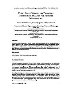
our approach: skip the dimensionality reduction
PCA 15
Regression 15
15
10
10
5
5
10
5
0 0
0
−5
−5
−5
−10
−15 15 10
15 5
10 0
−10
−10
5 0
−5 −5
−10
−10 −15
−15
−15 −15
−10
−5
0
5
10
15
−15 −15
−10
−5
0
5
10
15
4
our approach: skip the dimensionality reduction
PCA 15
Regression 15
15
10
10
5
5
10
5
0 0
0
−5
−5
−5
−10
−15 15 10
15 5
10 0
−10
−10
5 0
−5 −5
−10
−10 −15
−15
−15 −15
−10
−5
0
5
10
15
−15 −15
−10
−5
0
5
10
15
Regression is cheap (fast iterative or stochastic methods).
PCA is a major computational bottleneck.
4
our approach: skip the dimensionality reduction
Single-shot iterative algorithm 15
15
10
10
5
5
0
0
−5
−5
−10
−10
−15 15
−15 15 10
15 5
10 0
5 0
−5 −5
−10
−10 −15
−15
10
15 5
10 0
5 0
−5 −5
−10
−10 −15
−15
5
our approach: skip the dimensionality reduction
Single-shot iterative algorithm 15
15
10
10
5
5
0
0
−5
−5
−10
−10
−15 15
−15 15 10
15 5
10 0
5 0
−5 −5
−10
−10 −15
−15
10
15 5
10 0
5 0
−5 −5
−10
−10 −15
−15
Final algorithm just uses a few applications of any fast, black-box regression routine.
5
formal setup
Standard Regression: Given: A, b Solve: x∗ = arg minx ∥Ax − b∥2
6
formal setup
Standard Regression: Given: A, b Solve: x∗ = arg minx ∥Ax − b∥2 Principal Component Regression: Given: A, b, λ Solve: x∗ = arg minx ∥Aλ x − b∥2
6
formal setup
Standard Regression: Given: A, b Solve: x∗ = arg minx ∥Ax − b∥2 Principal Component Regression: Given: A, b, λ Solve: x∗ = arg minx ∥Aλ x − b∥2
data points
features
A
left singular vectors singular values σ1 σ2
=
U
Σ
σd-1 σd
right singular vectors
VT
6
formal setup
Standard Regression: Given: A, b Solve: x∗ = arg minx ∥Ax − b∥2 Principal Component Regression: Given: A, b, λ Solve: x∗ = arg minx ∥Aλ x − b∥2
data points
features
Aλ
left singular vectors singular values σ1 σ2
= Uλ
Σkλ
right singular vectors
VλT
σd-1 σd
6
formal setup
Singular values of A 20
σi2
15
10
5
0
0
100
200
300
400
500
600
700
800
900
1000
i 7
formal setup
Singular values of A 20
“Signal” σi2
15
10
“Noise”
5
λ 0
0
100
200
300
400
500
600
700
800
900
1000
i 7
formal setup
Singular values of Aλ 20
“Signal” σi2
15
10
“Noise”
5
λ 0
0
100
200
300
400
500
600
700
800
900
1000
i 7
formal setup
Principal Component Regression (PCR): Goal: x∗ = arg minx ∥Aλ x − b∥2 Solution: x = (ATλ Aλ )−1 ATλ b What’s the computational cost?
8
naive pcr runtime
Cost of computing Aλ (PCA): ≈ O(nnz(A)k + dk2 ).
9
naive pcr runtime
Cost of computing Aλ (PCA): ≈ O(nnz(A)k + dk2 ). k is the number of principal components with value > λ.
9
naive pcr runtime
Cost of computing Aλ (PCA): ≈ O(nnz(A)k + dk2 ). k is the number of principal components with value > λ. Cost of evaluating x = (ATλ Aλ )−1 ATλ b (regression): ≈ O(nnz(A) ·
√ κ).
9
naive pcr runtime
Cost of computing Aλ (PCA): ≈ O(nnz(A)k + dk2 ). k is the number of principal components with value > λ. Cost of evaluating x = (ATλ Aλ )−1 ATλ b (regression): ≈ O(nnz(A) ·
√ κ).
For PCR, k is large, κ is small (Aλ is well conditioned). 9
our goal
Goal: Remove bottleneck dependence on k
10
reason for hope?
Optimistic observation: PCA computes too much information.
11
reason for hope?
Optimistic observation: PCA computes too much information.
x∗ = (ATλ Aλ )−1 ATλ b =
11
reason for hope?
Optimistic observation: PCA computes too much information.
x∗ = (ATλ Aλ )−1 ATλ b = (AT A)−1 ATλ b
11
reason for hope?
Optimistic observation: PCA computes too much information.
x∗ = (ATλ Aλ )−1 ATλ b = (AT A)−1 ATλ b
Don’t need to compute Aλ (which incurs a k dependence) as long as we can apply it to a single vector efficiently.
11
reason for hope?
It’s very often more efficient to apply a matrix function once than compute the matrix function explicitly.
12
reason for hope?
It’s very often more efficient to apply a matrix function once than compute the matrix function explicitly. ∙ (AT A)x, (AT A)2 x, or (AT A)3 x
12
reason for hope?
It’s very often more efficient to apply a matrix function once than compute the matrix function explicitly. ∙ (AT A)x, (AT A)2 x, or (AT A)3 x ∙ A−1 x
12
reason for hope?
It’s very often more efficient to apply a matrix function once than compute the matrix function explicitly. ∙ (AT A)x, (AT A)2 x, or (AT A)3 x ∙ A−1 x ∙ exp(A) . . . many more
12
reason for hope?
It’s very often more efficient to apply a matrix function once than compute the matrix function explicitly. ∙ (AT A)x, (AT A)2 x, or (AT A)3 x ∙ A−1 x ∙ exp(A) . . . many more
Why not Aλ ?
12
main result
Theorem (Main Result) There’s an algorithm that approximately applies ATλ to any vector b using ≈ log(1/ϵ) well conditioned linear system solutions.
13
main result
Theorem (Main Result) There’s an algorithm that approximately applies ATλ to any vector b using ≈ log(1/ϵ) well conditioned linear system solutions.
PCR in ≈ O(nnz(A) ·
√
κ) time.
13
decomposing matrix
Goal: Apply ATλ quickly to any vector.
14
decomposing matrix
Goal: Apply ATλ quickly to any vector. 20
σi2
15
Spectrum of Aλ
10
5
λ 0
0
100
200
300
400
500
600
700
800
900
1000
i 14
decomposing matrix
50
AλT = SAT
45 40 35
Spectrum of A
σi2
30 25 20 15 10 5 0
0
100
200
300
400
500
600
700
800
900
1000
i
1.5
1
Spectrum of S
0.5
0
−0.5
0
100
200
(large σi)
300
400
500
i
600
700
800
900
1000
(small σi)
14
decomposing matrix
ATλ b = SAT b 1.5
1
Spectrum of S
0.5
0
−0.5
0
100
200
(large σi)
300
400
500
i
600
700
800
900
1000
(small σi)
How do we apply S to AT b? 15
decomposing matrix
How do we apply S to AT b? This is actually a common task.
16
decomposing matrix
How do we apply S to AT b? This is actually a common task. ∙ Saad, Bekas, Kokiopoulou, Erhel, Guyomarc’h, Napoli, Polizzi, others: Applications in eigenvalue counting, computational materials science, learning problems like eigenfaces and LSI, etc.
16
decomposing matrix
How do we apply S to AT b? This is actually a common task. ∙ Saad, Bekas, Kokiopoulou, Erhel, Guyomarc’h, Napoli, Polizzi, others: Applications in eigenvalue counting, computational materials science, learning problems like eigenfaces and LSI, etc. ∙ Tremblay, Puy, Gribonval, Vandergheynst: “Compressive Spectral Clustering” ICML 2016. 16
a first approximation
We turn to Ridge Regression, a popular alternative to PCR:
17
a first approximation
We turn to Ridge Regression, a popular alternative to PCR: Goal: x∗ = arg minx ∥Ax − b∥2 + λ∥x∥2 . Solution: x∗ = (AT A + λI)−1 AT b.
17
a first approximation
We turn to Ridge Regression, a popular alternative to PCR: Goal: x∗ = arg minx ∥Ax − b∥2 + λ∥x∥2 . Solution: x∗ = (AT A + λI)−1 AT b.
Claim:
R = (AT A + λI)−1 AT A coarsely approximates S.
17
a first approximation
Singular values of S: σi (S) =
1 0
if σi2 (A) ≥ λ, if σi2 (A) < λ.
18
a first approximation
Singular values of S: σi (S) =
1 0
if σi2 (A) ≥ λ, if σi2 (A) < λ.
Singular values of R = (AT A + λI)−1 AT A: σi (R) =
σi2 (A) σi2 (A) + λ
18
a first approximation
Singular values of S: σi (S) =
1 0
if σi2 (A) ≥ λ, if σi2 (A) < λ.
Singular values of R = (AT A + λI)−1 AT A: 1 if σ 2 (A) >> λ, 2 σ (A) i ≈ σi (R) = 2 i σi (A) + λ 0 if σ 2 (A)