ASHRAE Journal
Pumps
Wire-to-Water Efficiency Of Pumping Systems By James B. (Burt) Rishel, P.E. Fellow/Life Member ASHRAE
I
n the past, wire-to-water efficiency of pumping systems was seldom considered except for very large pumps where the wire-to-water efficiency of the pump-motor combination was of significant importance. The advent of higher electrical costs in conjunction with the emergence of the variable speed drive and digital electronics has made wire-to-water efficiency invaluable for smaller pumping systems.
Of what value is wire-to-water efficiency? This procedure is the best method of determining the overall efficiency of a pumping system. It includes the efficiency of the pump, the pump motor, that of any variable speed drive involved, and, on multiple pump systems, it takes into account the losses in the piping fittings that surround the pumps. It enables an engineer or operator to evaluate the total pumping installation. An extensive review of this efficiency will be made later. Basically, wire-to-water efficiency is the energy that is imparted to the water divided by the energy that came in over the electrical wires. It is work done divided by work applied. The wire-to-water efficiency of a single pump, constant speed pumping system is: WWE = E
m
× E × 100% p
(1)
where, Em = Motor Efficiency as a fraction Ep = Pump Efficiency as a fraction The wire-to-water efficiency of pumpmotor combinations will vary from less than 20% for small, fractional horsepower, circulating pumps to more than 85% for large pumps and motors. Therefore, it is beneficial to consolidate pumping func40
ASHRAE Journal
tions where it is economically feasible. The wire-to-water efficiency of a multiple pump, constant speed pumping system is: H – H s pf WWE = H
E × E m p s
(2)
where, Hs = Total friction loss of the water system in feet of head Hpf = Friction loss in feet of head of the pump fittings including strainers, check valve, shut-off valves, and the header losses that direct the flow into and from each pump. The wire-to-water efficiency of a singlepump, variable-speed pumping system is: (3) WWE = E × E × 100% ws
p
where, Ews = The wire-to-shaft efficiency of the motor variable-speed drive combination expressed as a fraction. The wire-to-water efficiency of a variable-speed pumping system with multiple pumps is: H – H E × E s pf ws p WWE = H s
(4)
There may be some question concerning the inclusion of the fitting loss, Hpf , in the formula for wire-to-water efficiency for multiple pumping systems. It must be included, as it is impossible to program the pumps on and off on multiple pumping systems without considering the fitting loss, because the flow through each pump is a fraction of the total system flow. The loss through the pump fittings affects the overall wire-to-water efficiency. If pumps are operated above their design flow, the fitting loss will be much greater than at design flow. Basically, the loss through fittings varies generally with the square of the flow. It is ignored on singlepump systems, because the flow through the pump is the same as the total system flow. The wire-to-shaft efficiency of the motor and the variable-speed drive is one of the most important, and yet, difficult efficiencies to generate. It is not only the efficiency of the motor multiplied by the efficiency of the drive. The efficiency of the motor is dependent upon the load imposed upon it. The load on a motor at reduced speed is determined by the system head curve or the system head area. Companies who provide wire-to-water efficiency calculations understand these requirements and provide the software for the calculation of wire-to-water efficiency once the parameters of the water system and its pumping equipment have been determined. Other than the generation of the term, Ews, the equations for wire-to-water efficiency are fairly straightforward. The calculation of wire-to-water efficiency for a About the Author James B. (Burt) Rishel, P.E., has formed a consulting company, Pumping Solutions LLC, Cincinnati.
w w w. a s h r a e j o u r n a l . o r g
April 2001
ASHRAE Journal Coil, Coil Piping, and Control Valve Loss
35 ft System Friction
10 Floors 160 gpm ea.
Coil, Coil Piping, and Control Valve Loss
25 ft 70 60 System Head — ft
25 ft
50 40% Load 40
System Friction
35 ft System Friction
10 Floors 160 gpm ea.
30 20
Two-Way Valves
0 0
Chiller
Two-Way Valves
Constant Differential Pressure
10
400
800
1200
1600
Chiller
Flow — gpm 8 ft
8 ft
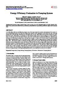
Figure 1: Model building for system head area evaluation.
prospective system can be difficult if inadequate system analysis is used. The following discussion of a relatively simple chilled water system will demonstrate this complexity. The equation for system head for any water system is: Q System head, ft = C + H × h f Q d
n
(5)
where, Ch = Any constant head in feet such as cooling tower height or constant pressure at the end of a chilled or hot water loop, Hf = Calculated, variable friction in feet of head for the water system at design flow, Qd, Q = The flow at any other quantity in the water system Qd = Design flow for the water system in gpm n = Friction coefficient for the water system. This exponent is normally 2, but it has proved to be a variable. (See the following explanation.) System Analysis For many years, it was assumed that the system head curve for any installation had an exponent of two or that the head varied as the square of the flow. Williams-Hazen Equation friction calculations were based upon an exponent of 42
ASHRAE Journal
Figure 2: Uniform system head curve for model Figure 3: Uniformly loaded building, building. 40% load on each air-handling unit. Coil, Coil Piping, and Control Valve Loss
25 ft
10 Floors 160 gpm ea.
35 ft System Friction
Coil, Coil Piping, and Control Valve Loss
25 ft
35 ft System Friction
10 Floors 160 gpm ea.
Two-Way Valves
Two-Way Valves
Chiller
Chiller 8 ft
8 ft
Figure 4: Non-uniformly loaded building, air-handling units close to pumping source, fully loaded.
Figure 5: Non-uniformly loaded building, air handling units far from pumping source, fully loaded.
1.85, and a review of Darcy Wiesbach Equation friction data indicates an exponent of around 1.90. All of these older system curves were based upon a uniform loading throughout the water system. In real life, this is seldom found. A system head area with the exponent varying from 0.37 to 3.7 more truly represents the relationship between the system flow and system head. So far, this article pertains to all water systems. The following is based upon a loop-type, chilled water
system. This system is described in Figures 1 through 8. Assume that the water system is as shown in Figure 1 for a building with 10 floors of cooling units, each requiring 160 gpm (10 L/s). Also assume that the required head for each floor cooling unit coil, control valve, and piping is 25 feet of head (75 kPa). Further assume that the friction loss in the building headers is 35 feet (105 kPa). The uniform system head curve, assuming a coefficient of 1.85, is
w w w. a s h r a e j o u r n a l . o r g
April 2001
ASHRAE Journal 60
Loads Active Far From Water Source
Bldg. B
50 Large Loop Loss
System Head — ft
40
30 20
Loads Active Near Water Source Uniform System Head Curve
Bldg. A
10
Central Small Chilled Water Plant Loop Loss
0 0
267
533 800 1067 1333 1600 Building Flow — gpm
Figure 7: Loop loss variation in central plant installation.
Figure 6: System head area caused by non-uniform flow in building.
described in Figure 2. This assumes that all 10 floors of cooling units vary their loads uniformly as shown in Figure 3 at 40% load on the system. Now let the load on the system remain at 40% with only the four bottom floors active as indicated in Figure 4. The overall friction loss will now be less than that for the uniformly loaded building. Next, let the top four floors be fully loaded as shown in Figure 5. Now the friction loss will be greater than the uniformly loaded building at 40% load. If this procedure were followed from one to ten floors, the actual system head area for this building would be as described in Figure 6. Most buildings do not have as broad a system area as this. This is a demonstration of the complexity of system evaluation with a relatively simple building. When a group of buildings is evaluated, the calculations become more challenging. Figure 7 illustrates a small campus of seven buildings divided into two distribution loops. Assume that the building of Figure 1 does not have an internal chiller plant and is located at two different points on this installation, namely at Point A and Point B. The system head area for the building at Point A will be substantially the same as Figure 6. This will not be the case when the building is located at Point B. Assume that the friction loss in the supply and return loops between the buildings and the central plant is thirty feet at design load on all of the five buildings. We now have two conditions to consider for Building B, one with all of the other four buildings at design load and, secondly, with no load on these four buildings. The result is Figure 8. The system head area has broadened appreciably, and it is obvious that substantial energy will be wasted if the pump selection and control are not considered carefully. It may be argued that this is an unusual situation, but the author has found many similar conditions over the past 30 years. This type of head variation has been masked in the past by balancing out any so-called over pressures. The load variation in the campus-type application will complicate the wire-to-wa44
ASHRAE Journal
ter efficiency evaluation. Instead, just the simple building itself as shown in Figure 1 will be used in the following discussion of wire-to-water efficiency. Wire-To-Water Efficiency Analysis Assume that the above building has its own chilled water pumps. Three pumps will be used with a 50% capacity each of 800 gpm (50 L/s). The pump head will be the building head of 60 feet (179 kPa) plus the pumping system friction loss, Hpf, of 8 feet (24 kPa) for a total head of 68 feet (203 kPa). Wire-to-water efficiency calculations will now be run for the building at system head curve coefficients of 0.37, 0.74, 1.11, 1.48, 1.85, and 2.59, and 3.70 using Equation 4. These exponents were selected to cover the entire system head area incrementally. This will provide us with the wire-to-water efficiency of the pumping system with one, two, and three pumps operating under different load conditions in the building. The actual calculations will not be shown, as there is not room in this short article for them. Also, the results of the wire-to-water efficiency evaluation are what should be emphasized here. The results of the computer runs at the water system exponents listed earlier are summarized in Tables 1 and 2. Table 1 describes the variation in wire-to-water efficiency with changes in the system head curve exponent while Table 2 indicates the variation in the number of pumps that should be operated with changes in the system head curve exponent. The pumps were selected so that two pumps could operate this chilled water system at 100% load. Table 2 demonstrates that although this is possible, it is more efficient to run all three pumps at loads in excess of from 1,280 to 1,600 gpm (81 to 101 L/s) depending upon the system coefficient. The Tables 1 and 2 also demonstrate the variation in wire-towater efficiency and optimum number of pumps that should be operated on this particular chilled water system. Figure 9 describes the variation of the wire-to-water efficiency with the system head coefficient for one, two, and three pumps operating. Actually, this is a two dimensional description of threedimensional surfaces. Plotting system flow, wire-to-water efficiency, and system head on the x, y, and z axes results in the three-dimensional surfaces shown in Figure 10.
w w w. a s h r a e j o u r n a l . o r g
April 2001
Pumps System Head Coefficient
System Head Coefficient
System Flow n=0.37 n=0.74 n=1.11 n=1.48 n=1.85 n=2.59 n=3.70 (gpm)
System Flow n=0.37 n=0.74 n=1.11 n=1.48 n=1.85 n=2.59 n=3.70 (gpm)
160
37.8
38.5
38.7
38.8
38.9
38.9
38.9
160
1
1
1
1
1
1
1
320
59.6
59.5
59.0
58.2
58.2
57.7
57.5
320
1
1
1
1
1
1
1
480
67.2
65.5
63.8
62.5
61.3
59.8
59.0
480
1
1
1
1
1
1
1
640
66.6
64.1
61.6
59.8
59.5
58.2
58.0
640
1
1
1
1
2
2
2
800
64.9
64.8
64.5
63.8
62.9
62.1
61.1
800
2
2
2
2
2
2
2
960
68.1
67.4
67.0
66.1
66.0
63.9
62.2
960
2
2
2
2
2
2
2
1,120
69.0
68.2
67.6
66.8
66.2
64.6
62.4
1,120
2
2
2
2
2
2
2
1.280
68.5
67.9
67.2
66.6
66.2
65.9
65.3
1.280
2
2
2
2
3
3
3
1,440
68.3
68.9
68.1
68.0
68.1
67.8
67.4
1,440
3
3
3
3
3
3
3
1,600
69.4
69.4
69.4
69.4
69.4
69.4
69.4
1,600
3
3
3
3
3
3
3
Table 1: Wire-to-water efficiency variation. 90
Table 2: Number of pumps running. Three pumps n = 0.37
Two pumps
One pump
Loads Active Far from Water Source and Other Building Fully Loaded
70 n = 0.37
80
n = 0.37
Building Head — ft of water
60 70
n = 3.7
n = 3.7
60 n = 3.7 50
50
40
30 40 20
10 0
Loads Active Near Water Source and Other Buildings Inactive 267
533 800 1067 Building Flow — gpm
1333
1600
30
0
200
400
600
800 1000 1200 System flow — gpm
1400
1600
Figure 8: System head area caused by non-uniform flow in Building B and other buildings.
Figure 9: Wire-to-water efficiency areas for model building.
How can one possibly develop this technology, practically, into the actual control of pumps for such a relatively simple water system, let alone the complexity of a multiple building system as shown in Figure 7? The advent of digital computer technology will enable software engineers to generate the equations for the surfaces shown in Figure 10 and to define the points of intersection at which pump operation should transition from one to two to three pumps automatically regardless of the system head curve coefficient. Practically, plant operators can program their pumps through the observation of the electrical consumption of the pumping system as loads vary on the
water system. Although no great variations in energy exist for this model building with three 20 hp (15 kW) pumps, consider the larger building complexes where as many as six 800 hp (597 kW) pumps are required to distribute many thousands of gallons per minute. The actual use of wire-to-water efficiency in the operation of water systems has proved to be of great value for operating engineers. By using Equation 5, the operating wire-to-water efficiency of a water system can be displayed on the operator’s monitor where it can be checked to ensure that the correct number of pumps is in operation. Any of the techniques of
April 2001
ASHRAE Journal
45
information storage, retrieval, and manipulation can be used to ensure that the pumping system is operating at peak, overall efficiency. Past performance comparisons can be made to determine the need for pump service and inspection. A particular installation where this technology is used is the central chilled water plant at Harvard University. The transition points in multiple pump systems are very important in pumping a water system efficiently, and they can be checked easily to ensure that the calculated program is adequate for the actual system. This eliminates operation at low and high flows in the individual pumps. This, in turn, reduces noise and unnecessary wear in the pumps themselves. The pumps are operated as closely as possible to their best efficiency curve. Variable speed pumping systems using this technology are known to operate for many years without any structural damage to the pumps themselves. This demonstrates that wire-to-water efficiency technology is useful through digital computer programming for even relatively small systems. As more companies become proficient in this software, it will become standard for any water system with multiple loads and total pump horsepower in excess 50 hp (37 kW). The previously mentioned variation in wire-to-water efficiency for individual pump-motor combinations from less than
Wire-to-water efficiency (%)
ASHRAE Journal One pump 70 60 50 40 30 20 10 0
Two pumps Three pumps
200 400 Sy 600 ste m flo 800 w (gp m) 1000
1200
60 50 ) 40 d (ft 30 ea 1400 h 20 1600 10 stem 0 Sy
Figure 10: Three-dimensional figure for wire-to-water efficiency.
20% for small pumps to more than 85% for large pumps demonstrates the need to track wire-to-water efficiency for most pumping systems.
Apply Yourself
IAQ Applications
Advertisement for the print edition formerly in this space.
IAQ Applications is distributed quarterly to scores of IAQ professionals. Its goal is to breach the gap between research and application, providing practical answers to today’s most pressing IAQ issues.
! Columns from medical and industry experts ! Peer-screened articles on the latest IAQ topics ! IAQ columns by chairs of ASHRAE standards committees Subscription Rates: 1-year (4 issues): $59 ($39 ASHRAE member price) Outside U.S./Can add $9 for postage. Product Code: 40221 To Order: ASHRAE Customer Service (800) 5-ASHRAE in the U.S. or Canada (404) 636-8400 worldwide M-F 8am-5pm (EST) Fax: (404) 321-5478 E-mail:
[email protected] Order on-line at www.ashrae.org
46
ASHRAE Journal
w w w. a s h r a e j o u r n a l . o r g
April 2001