USING SATELLITE-BASED RAINFALL ESTIMATES FOR RUNOFF MODELLING WITH THE REW APPROACH: THE CASE OF UPPER GILGEL ABAY CATCHMENT

ASSAYEW NEBERE AMBAW February, 2016

SUPERVISORS: Dr.Ing. T.H.M. Rientjes Ir. G.N. Parodi

Using satellite-based rainfall estimates for runoff modelling with the REW approach: the case of Upper Gilgel Abay catchment ASSAYEW NEBERE AMBAW Enschede, The Netherlands, February, 2016 Thesis submitted to the Faculty of Geo-Information Science and Earth Observation of the University of Twente in partial fulfilment of the requirements for the degree of Master of Science in Geo-information Science and Earth Observation. Specialization: Water Resources and Environmental Management

SUPERVISORS: Dr.Ing. T.H.M. Rientjes Ir. G.N. Parodi THESIS ASSESSMENT BOARD: Dr. M.W. Lubczynski (Chair) Prof. P. (Paolo). Regianni (External Examiner, University of Siegen)

DISCLAIMER This document describes work undertaken as part of a programme of study at the Faculty of Geo-Information Science and Earth Observation of the University of Twente. All views and opinions expressed therein remain the sole responsibility of the author, and do not necessarily represent those of the Faculty.

ABSTRACT A physically based hydrological modeling approach, Representative elementary watershed (REW), has been applied to the Upper Gilgel Abay catchment which is the largest contributor to the inflow to Lake Tana, the source of Blue Nile River. Application and evaluation of performances of satellite rainfall estimates (SRE) for representing the spatial and temporal variability of rainfall in data poor catchments such as Upper Gilgel Abay is vital. Rainfall variability was reported within Upper Gilgel Abay catchment between mountainous areas and flat areas close to the Lake. The important component which is associated with variability of rainfall is the runoff dynamics and generation mechanisms in Upper Gilgel Abay catchment. Hence, the focus of this study was to test the effectiveness satellite rainfall estimates at high spatial and temporal resolutions for simulating spatial dynamics of runoff in Upper Gilgel Abay catchment. The study period of 2006-2010 was used for downloading the 1-hr temporal and 8 km × 8 km spatial resolution CMORPH data (selected from SREs), and extracting SRE. SREs are constrained for use because of the systematic and random errors over space and time. For correcting the systematic biases, time and space variant bias correction algorithm was applied for a time window of 7 days and a minimum rain accumulation of 5 mm with in these days. Bias correction selected for this study aimed at correcting both in space and time domains. To estimate potential evapotranspiration for model inputs PenmanMonteith equation was calculated from climatological and field measurements. TARDEM software was used in the model for extracting the REWs and performing hydro processing from SRTM DEM with a resolution of 90 m. The model was calibrated for the period 2006-2008 using rainfall data from the rain gauges. Calibration was conducted in trial and error through parameter optimization. After getting the better performing model results the precipitation forcing was replaced with CMORPH inputs. Objective functions like NS, RVE and Y were applied to assess how well the stream flows were reproduced in simulations. Hourly CMORPH based simulations were used as modeling time step to simulate the diurnal variability of streamflow in Upper Gilgel Abay catchment. The result was evaluated through visual inspection and Exceedance probability plots. Based on modeling results, objective function values for calibration are 0.71 for NS, 4.07% for RVE and 0.68 for Y. Values as such indicate a satisfactory model performance. The sensitivity analysis results show hydraulic conductivities, soil porosity and depth of saturated subsurface flow layer are highly sensitive in affecting the simulation results. Objective function values of 0.57 for NS, 0.80% for RVE and 0.56 for Y was reported while using CMORPH SRE inputs instead of Insitu rainfall estimates. Thus, Insitu based simulation has better reproduced the measured streamflow hydrograph than CMORPH based streamflow simulations. A validation result of 0.62 for NS, 9.59% for RVE and 0.57 for Y was found and the validation results deteriorated from the calibration results. The daily aggregated CMORH simulation suppresses the high peak flows and low flows when compared to the hourly CMORPH. Regarding saturated excess overland flow, the spatial differences in signals identified in Upper Gilgel Abay catchment where REWs close to the river reaches and areas of flat terrain contribute higher to streamflow by saturation excess overland. Overall, the performance of SREs based streamflow simulations was able to capture the shape of stream flow hydrograph measured. Model recalibration with SRE forcing might improve the model performance even better. KEY WORDS: REW; CMORPH; Satellite rainfall estimates; runoff; modelling

ACKNOWLEDGEMENTS First and foremost I would like to thank God for his mercy all the way through my life. I would like to express my sincere gratitude to the government of the Netherlands for providing me this great opportunity to study under the Netherlands fellowship program. I consider it a profound pleasure to express my deep sense of indebtedness, gratitude and profound thanks to first supervisor Dr.Ing T.H.M. Rientjes, for his valuable comments and guidance throughout the research. His comments and helpful guidance gave me a chance to explore further. I have learned a lot from him. I would also like to give great gratitude to Ir. G.N. Parodi my second supervisor, for his supportive and valuable comments. I would thankfully acknowledge Ministry of Water Resources and Bahir Dar Meteorological Services Agency in Ethiopia for providing hydro-meteorological data for the study. I would gratefully like to acknowledge University of Gondar for allowing me to pursue my studies abroad. I would also like to extend my deepest gratitude to my friends, colleagues in ITC, WREM department staffs in ITC, and GeES Department staffs in University of Gondar. I am forever grateful to my beloved Father Nebere Ambaw. He had always been the constant source of my strength and hope in every aspect of my life. My special heartfelt gratitude also goes to my beloved wife Sosina Mihret, my mother Simegn Alemu and my brother Getaye Nebere for their affection and encouragement.

TABLE OF CONTENTS 1.

Introduction ............................................................................................................................................. 1 1.1.

Background .....................................................................................................................................................................1

1.2.

Problem Statement ........................................................................................................................................................2

1.3.

Main objective ................................................................................................................................................................2

1.3.1. 1.3.2.

2.

1.4

Relevance of the study ..................................................................................................................................................3

1.5

Thesis outline ..................................................................................................................................................................3

study area and data availability ...............................................................................................................4 2.1.

Study area description ...................................................................................................................................................4

2.1.1. 2.1.2. 2.1.3. 2.2.

4.

Data Availability .............................................................................................................................................................7

Insitu measurement............................................................................................................................7

2.2.2.

Remote sensing data ..........................................................................................................................9

Meteorological Variables ...............................................................................................................................7 Hydrological Data ...........................................................................................................................................8

Literature review .................................................................................................................................... 10 3.1.

Sattelite rainfall estimates as forcing for Modeling runoff ................................................................................... 10

3.2.

Runoff processes ......................................................................................................................................................... 11

3.3.

Hydrograph components ........................................................................................................................................... 13

Methodology .......................................................................................................................................... 14 4.1.

Methodological approach .......................................................................................................................................... 14

4.2.

Processing satellite rainfall estimates ....................................................................................................................... 15

4.3.

Comparison of stream flow simulation using rainfall forcing of daily and hourly CMORPH ..................... 16

4.4.

Filling in techniques used for missing gauge measurements ............................................................................... 16

4.5.

Penman-Monteith equation for Potential Evaporation ....................................................................................... 17

4.6.

Digital elevation model (DEM) processing ............................................................................................................ 18

4.7.

Model description ....................................................................................................................................................... 19

4.8.

Balance equations at the REW-scale ....................................................................................................................... 21

4.9.

Parameters and variables............................................................................................................................................ 22

4.10.

Evaluation of model performance ........................................................................................................................... 23

4.2.1. 4.2.2.

5.

Geographical location and topography ..........................................................................................4 Climate .................................................................................................................................................5 Land use/Land cover, Soil and Geology........................................................................................6

2.2.1.

2.2.1.1. 2.2.1.2.

3.

Specific objectives ..............................................................................................................................2 Research questions .............................................................................................................................3

Extraction of SREs ......................................................................................................................... 15 Bias correction scheme................................................................................................................... 15

Result and Discussion ........................................................................................................................... 24 5.1.

Performance of satellite rainfall estimates (SREs) in Upper Gilgel Abay Catchment .................................... 24

5.1.1. 5.1.2. 5.2.

Performance of CMORPH ........................................................................................................... 24 Effects of Bias correction .............................................................................................................. 26

REW modelling ........................................................................................................................................................... 27

5.2.1.

Calibration and Validation ............................................................................................................. 27

i

5.2.1.1. 5.2.1.2. 5.2.1.3.

6.

ii

Model calibration ......................................................................................................................................... 28 Sensitivity Analysis ...................................................................................................................................... 29 Model Validation ......................................................................................................................................... 30

5.3.

Runoff simulation with sattelte rainfall estimates forcing ................................................................................... 31

5.4.

Identification of major runoff source with in the catchment ............................................................................. 32

5.5.

Comparision of high temporal resolution (hourly) and daily forcing on runoff simulation ......................... 35

5.6.

Discussion .................................................................................................................................................................... 37

Conclusion and Recommendation ........................................................................................................ 40 6.1.

Conclusions .................................................................................................................................................................. 40

6.2.

Recommendations ...................................................................................................................................................... 41

LIST OF FIGURES Figure 1: Location of Upper Gilgel Abay catchment ..............................................................................................4 Figure 2: Elevation map of Upper Gilgel Abay catchment ....................................................................................5 Figure 3: Basin averaged daily rainfall of Upper Gilgel Abay catchment (2006-2010).......................................5 Figure 4: Average daily temperature of Upper Gilgel Abay catchment (2006-2010) .........................................6 Figure 5: Location of meteorological and gauging stations considered in Upper Gilgel Abay catchment .....8 Figure 6: Annual rainfall of Upper Gilgel Abay catchment for meteorological stations ...................................8 Figure 7: Discharge measurement taken in the outlet of Upper Gilgel Abay catchment ..................................9 Figure 8: classification of runoff generation mechanisms (Source: Tarboton (2003) adapted from (Beven, 2000)). ........................................................................................................................................................................... 11 Figure 9: Typical surface with saturation excess (exfiltration) in the Upper Gilgel Abay catchment (photo: Dr.Ing. T.H.M. Rientjes). .......................................................................................................................................... 12 Figure 10: stream flow hydrograph (from public resource GeogOnline) ......................................................... 13 Figure 11: Flowchart showing the procedures and methods............................................................................... 14 Figure 12: Characteristics of the hypothetical reference crop (Source: (Allen, 1998)) .................................... 17 Figure 13: REWs delineated with Second Strahler order ..................................................................................... 18 Figure 14: Discretization of the Upper Gilgel Abay river catchment in to 33 REWs (Left) and 173 REWs (Right) based on Strahler order used ....................................................................................................................... 19 Figure 15: Three-dimensional view of REW model ( Source:( Reggiani & Rientjes, 2005))......................... 20 Figure 16: REW cross-section and mass exchange terms (source: (Fenicia et al., 2005)) ............................... 20 Figure 17: Scatter plots of CMORPH and gauge daily rainfall (2006-2010) ..................................................... 25 Figure 18: Whisker plot showing comparison of BF’S obtained from 7 days sampling window (2006-2010) ....................................................................................................................................................................................... 26 Figure 19: Hydrograph showing the calibration result for 2006-2008 ............................................................... 29 Figure 20: validation hydrograph for the year 2009 .............................................................................................. 30 Figure 21: Streamflow simulation with bias orrected CMORPH rainfall estimates (2006-2010) .................. 31 Figure 22: Stream flow simulation with bias corrected CMORPH rainfall estimate (left; for the year 2008; and right; 2010) ........................................................................................................................................................... 32 Figure 23: Average Saturation excess thickness (mm) for REWs for wet season (months of June, July, August and September 2006-2008) per day............................................................................................................ 33 Figure 24: major runoff generation (saturation excess) source REWs .............................................................. 33 Figure 25: Simulated saturated excess overland flow thickness for REW 4, REW 13, and REW 25........... 34 Figure 26: Correlation of REW average daily rainfall and Simulated saturated excess overland flow for REW 4, REW 13, and REW 25 ............................................................................................................................... 34 Figure 27: Comparison of hourly and the daily forcing on runoff simulation (June, July and August 2010) ....................................................................................................................................................................................... 35 Figure 28: Exceedance probability graph................................................................................................................ 36 Figure 29: Streamflow simulation with bias corrected CMORPH and Insitu rainfall estimates(2006-2008) ....................................................................................................................................................................................... 38

iii

LIST OF TABLES Table 1: Shows meteorological variables collected for this study.......................................................................... 7 Table 2: Summary of Mass balance equations in REW model (Reggiani & Rientjes, 2005) ........................... 21 Table 3: Summary statistics of gauge and CMORPH daily rainfall (2006-2010) .............................................. 24 Table 4: Summary statistics of CMORPH daily rainfall before and after TSV bias correction ..................... 27 Table 5: Sensitivity analysis (2006-2008).................................................................................................................. 30 Table 6: Performance of CMORPH on runoff simulation .................................................................................. 31

iv

USING SATELLITE-BASED RAINFALL ESTIMATES FOR RUNOFF MODELLING WITH THE REW APPROACH: THE CASE OF UPPER GILGEL ABAY CATCHMENT

1.

INTRODUCTION

1.1. Background Gilgel Abay catchment is of high interest to Ministry of Water Resources and Energy in Ethiopia because the basin is the head basin of the Upper Blue Nile and the largest contributor to Lake Tana which is responsible for some 30% of the mean annual lake inflow. Lake Tana is also the actual source of the Upper Blue Nile. Hence in recent years, the basin has received much attention from scientists. Most studies performed in the catchment are on rainfall-runoff modelling with the aim to better understand and simulate the hydrological regime. Applications are known for the HBV conceptual model by Wale (2008), Uhlenbrook et al. (2010) and Rientjes et al. (2011), and the semi-distributed conceptual model (TOPMODEL) by Moges (2008), Ahmed (2012) and Gumindoga (2015). Other studies known are on Lake Tana water balance modelling by Wale (2008) and Rientjes et al. (2011); and on hydrological impact assessments of land cover changes in Gilgel Abay by Moges (2008), Ahmed (2012) and Gumindoga (2015); Studies on climate change impact assessment on the hydrology of the catchment are by Abdo et al. 2009 and Yihun et al. 2013. Uhlenbrook et al. (2010) and Dessie et al. (2014) also applied a modified conceptual HBV model for better understanding of runoff processes in Gilgel Abay. Of major importance for modelling the relation between rainfall and runoff is the representation of rainfall over the catchment. Whereas assessing and representing rainfall variability is of high importance, unreliable and inaccurately observed rainfall may largely impact runoff simulation results. Aspects of rainfall variability in the Upper Gilgel Abay study area are reported by Haile et al. (2009), which reveals the variability between mountainous areas and flat areas close to the lake. In Upper Gilgel Abay catchment rain measuring stations are sparse in distribution and most are located outside the catchment. Observations from rain gauge stations are available daily with some of series incomplete. Hence, Satellite rainfall products can be considered as an option for rain gauge measurements. Satellite-based rainfall estimates have become available at high resolutions and are expected to offer an alternative to represent the variability rainfall estimates in data-sparse and ungauged catchments (Sawunyama & Hughes, 2008). In this regard, different products have been produced with the development of earth observation techniques. Rainfall variability is often influenced by nonlinear interactions between several factors like local variations of topography, the orientation of mountains and aspect (Haile et al., 2009). Terrain features also increases the variability of rainfall by means of processes such as rain shading and strong winds (Buytaert et al., 2006). Similarly, in Gilgel Abay catchment, Haile et al. (2009) revealed that the variation of rainfall is affected by topography and distance to the center of the Lake Tana. The study showed that in the basin less rainfall variation is observed over high-elevation areas than low-elevation areas. The variation in rainfall over the catchment also show temporal variability with frequent rainfall and convective activity mostly in the afternoon over the southern mountains and in the night over the southern part of the Lake Tana shore (Haile et al., 2009). Hence, in mountainous areas with a limited rain gauge network, as in the Gilgel Abay catchment, satellite-based rainfall estimation might provide information on rainfall occurrence, amount, and distribution at the highest spatial and temporal resolution (Anagnostou et al., 2010). On the other hand, land cover changes also affect the hydrology of a catchment by modifying evaporation and thereby influencing runoff generation (Cao et al., 2009). Here, some studies (e.g. Rientjes

1

USING SATELLITE-BASED RAINFALL ESTIMATES FOR RUNOFF MODELLING WITH THE REW APPROACH: APPLICATION TO THE UPPER GILGEL ABAY CATCHMENT

et al. 2011; Gumindoga et al. 2015) in Upper Gilgel Abay catchment focused on the impact of changes in land cover on stream flow and indicated the expansion of agricultural land and reduction of forest cover over the catchment (Li et al., 2012). Furthermore, the increasing demands of water resources and intensified land cover change calls for applying physically based distributed hydrological models which are capable of modeling the spatial and temporal dynamics of runoff behavior in catchments like Upper Gilgel Abay following the rainfall patterns. Therefore, there is a need to model the spatial and temporal variability of runoff in the catchment with satellite rainfall estimates (SRE) as a major input. 1.2.

Problem Statement

Rainfall-Runoff models are tools to represent and predict catchment processes. For runoff modeling, representing rainfall over time and space accurately is vital as it is one of the main causes for runoff generation. In Upper Gilgel Abay catchment rainfall stations are scarce and most are situated outside the catchment. Fortunately, with the development of earth observation technologies it is possible to use satellite rainfall estimates as forcing for hydrological modeling. As reported by scientific community, satellite rainfall estimates are contaminated with systematic errors also called bias both in temporal and spatial dimension. Hence, satellite products need to be bias corrected and their performance in representing rainfall should be evaluated before using such information for modeling work. Hence, the performance of bias corrected satellite products must be tested as forcing to simulate the runoff over long time series to have reasonable evaluation. Likewise runoff source areas (saturation excess) can be identified in response to rainfall variation over time and space for upper Gilgel Abay catchment. Assessing the dynamics of runoff behavior within the catchment by spatially distributed satellite rainfall forcing over space and time is a research gap identified and is one of the follow-up efforts of understanding the hydrology of the Upper Gilgel Abay catchment. The scientific problem here is the use of bias corrected satellite rainfall estimates which is available at high temporal (1-hr) and spatial (8 km × 8 km) resolution to be tested as forcing for the stream flow modeling in Upper Gilgel Abay catchment. 1.3. Main objective The main objective of this study is to test the effectiveness of bias corrected satellite rainfall estimates at high spatial and temporal resolutions for simulating spatial dynamics of runoff in Upper Gilgel Abay catchment. 1.3.1.

2

Specific objectives

o

To use bias corrected satellite rainfall estimates as forcing for the REW approach in Upper Gilgel Abay catchment.

o

To evaluate to what extent model performance is affected when satellite rainfall estimates are used instead of rainfall estimates from rain gauges.

o

To evaluate if major runoff source areas in the Upper Gilgel Abay catchment can be identified using REW approach.

o

To simulate runoff with hourly satellite-based rainfall and to evaluate how the diurnal rainfall cycle affects the stream flow hydrograph.

USING SATELLITE-BASED RAINFALL ESTIMATES FOR RUNOFF MODELLING WITH THE REW APPROACH: THE CASE OF UPPER GILGEL ABAY CATCHMENT

1.3.2.

Research questions

o

How accurate do satellite rainfall estimates represent rainfall for the modelling of runoff in Upper Gilgel Abay catchment?

o

Where are the major runoff source areas located in the Upper Gilgel Abay catchment?

o

Can locations of these areas be related to rainfall distribution?

o

How does the stream flow hydrograph change when hourly satellite-based rainfall data is used instead of data at the daily time step?

1.4 Relevance of the study This study is to evaluate if the REW with rainfall inputs from high spatial and temporal resolution satellite products can serve to better understand the dynamics of runoff behavior and runoff generation in Upper Gilgel Abay catchment. This modeling effort is a test case for the use of Satellite rainfall estimates (SREs) for modelling runoff source areas at sub-daily time scales. Such modelling is not demonstrated for the Gilgel Abay basin in Ethiopia. 1.5 Thesis outline The thesis has six chapters which include introduction, study area and data availability, literature review and model description, methodology, result and discussion and conclusion and recommendation. The Introduction chapter deals with a general background related to the study theme, justification and objectives for conducting this work. The relevance of the study is described in this chapter as well. The second chapter is about the description of the study area and the nature and quality of data. Descriptions are added on the collected data during a field work period and the satellite images that were used to achieve the objectives of the study. In the third chapter (literature review), related researches conducted in the study area and theme were reviewed. The fourth chapter describes the scientific methods which were applied for processing the data, model simulation procedures, analysis conducted, and the REW model and balance equations. Results and discussion, which addresses answers for the research questions, are presented in the fifth chapter. The final or sixth chapter forwards the conclusion and recommendations of the thesis work.

3

USING SATELLITE-BASED RAINFALL ESTIMATES FOR RUNOFF MODELLING WITH THE REW APPROACH: APPLICATION TO THE UPPER GILGEL ABAY CATCHMENT

2.

STUDY AREA AND DATA AVAILABILITY

2.1.

Study area description

2.1.1.

Geographical location and topography

Upper Gilgel Abay catchment is located in north-western Ethiopia with geographical coordinates of 10º56' to 11º51'N latitude and 36º44' to 37º23' E longitude. The catchment represents the gauged part of Gilgel Abay river basin. The total area of Upper Gilgel Abay catchment is 1657km2. The river originates in a place known as Gish Abay which is near a small town Sekela and it is the largest contributor to the inflow of Lake Tana (Rientjes et al., 2011). As shown in figure 2, the topography of catchment is characterized as rugged with highest elevation around 3504 meters and lowest around 1892 meters. Based on the information from SRTM Digital Elevation Map of the catchment, the south and south eastern part of the catchment is highland where mountain ranges are found and the Northern part of the catchment is characterized by relatively flat terrain.

Figure 1: Location of Upper Gilgel Abay catchment

4

USING SATELLITE-BASED RAINFALL ESTIMATES FOR RUNOFF MODELLING WITH THE REW APPROACH: THE CASE OF UPPER GILGEL ABAY CATCHMENT

Figure 2: Elevation map of Upper Gilgel Abay catchment 2.1.2.

Climate

The climate of Upper Gilgel Abay is dominated by the tropical highland monsoon. The main rainy season is from June to September during which south-west winds bring rains from the Atlantic Ocean. Some 7090 percent of mean annual rainfall occurs during this season (Taddele, 2009). As depicted in figure 3, the dry season starts in October and last till January with a short rainy period from February to May. In figure 3 average daily rainfall of the catchment is plotted and indicates the rainy seasons with their specific characteristics.

Figure 3: Basin averaged daily rainfall of Upper Gilgel Abay catchment (2006-2010)

5

USING SATELLITE-BASED RAINFALL ESTIMATES FOR RUNOFF MODELLING WITH THE REW APPROACH: APPLICATION TO THE UPPER GILGEL ABAY CATCHMENT

In the period of 2006 to 2010, the average daily rainfall of the catchment which is weighted using Thiessen polygons indicates clear spatial and temporal variability of rainfall. There is a decreasing trend of rainfall from south to north following topography. Average temperature measured in gauging stations (see Table 1) for 2006-2010 period shows small variation ( see figure 4). The diurnal range of temperature on average varies between 15 to 23 °C.

Figure 4: Average daily temperature of Upper Gilgel Abay catchment (2006-2010) 2.1.3.

Land use/Land cover, Soil and Geology

Most of the Upper Gilgel Abay catchment area is dominated by cropland with some woodlands and forested highlands. Besides the cultivated lands, the main land cover types are grassland, marshland, and forest with frequent patches of shrubs, eucalyptus woods and trees (Gumindoga et al., 2015). Land cover change studies in the Upper Gilgel Abay catchment show that forest land decreased from 50.9% in 1973 to 32.9% in 1986 (see Rientjes et al., 2011) . Agricultural land increased from 28.2% in 1973 to 40.2% in 1986. Forest on the other hand, decreased from 32.9% to 16.7% while agricultural land increased from 40.2% to 62.7 % for the 1986-2001 period (Rientjes et al., 2011). Soils are characterized by clay, clay loam and silt loam textures, each texture sharing similar proportions of the catchment area (Bitew & Gebremichael, 2011).The geology is characterized by scoraceous and fractured quaternary basalts underlying most part of the Upper Gilgel Abay catchment that show the highest groundwater potential as indicated by its high infiltration capacity and hydraulic properties. Many high discharging springs emerged from this rock unit and acts as the base flow for Gilgel Abay River, which drains to Lake Tana. Alluvial sediments are also found along the mouth of the Gilgel Abay river (after Kebede, 2013).

6

USING SATELLITE-BASED RAINFALL ESTIMATES FOR RUNOFF MODELLING WITH THE REW APPROACH: THE CASE OF UPPER GILGEL ABAY CATCHMENT

2.2.

Data Availability

2.2.1.

Insitu measurement

2.2.1.1.

Meteorological Variables

In the area inside and outside of the study catchment meteorological stations of different level are found (see figure 5) and collected from Regional Meteorological office in Bahir Dar. Based on the classification of the office there are principal, also termed level one stations, where precipitation, air temperature, wind speed, relative humidity and sunshine duration measurements are taken every three hours. Another set of stations are class three stations (ordinary), where precipitation and air temperature measurements are taken daily. In addition class four stations only serve for precipitation measurements at daily base. Based on this classification Adet, Dangila and Bahir dar are principal stations. Class three stations are Kidamaja and Wetet abay and class four stations includes Enjibara and Sekela. Table 1: Shows meteorological variables collected for this study Met. stations

longitude

latitude

Elevation

Rainfall

Temperature (max, min)

Relative humidity

Sunshine duration

Wind speed

Adet Bahir dar Dangila Sekella Enjibara Kidamaja Wetet Abay

332663.3 324455 262994.7 304679.7 270514 259513 287108.5

1245939.5 1281713 1244290.6 1214109.7 1213131 1216653 1257029.5

2180 1797 2119 2690 2540 1913 1920

x x x x x x x

x x x x x x x

x x x

x x x

x x x

“x” in the table indicates meteorological variables that were collected during fieldwork. As shown in table 1, measurement variables, geographic coordinates and elevation of seven meteorological stations selected for this study are shown. Measurement time series cover the period of 2006-2010. As shown in figure 5, most of the meteorological stations are outside the catchment. The gauging station where discharge measurements are taken is located in the Northern tip of the catchment.

7

USING SATELLITE-BASED RAINFALL ESTIMATES FOR RUNOFF MODELLING WITH THE REW APPROACH: APPLICATION TO THE UPPER GILGEL ABAY CATCHMENT

Figure 5: Location of meteorological and gauging stations considered in Upper Gilgel Abay catchment

After filling-in observed gaps in observation time series, annual rainfall of each meteorological station is calculated and shown in figure 6. Enjibara, Kidamaja and Sekela are stations which receive more than 2000 mm per annum. These stations are located in high altitude areas. The inter-annual distribution of rainfall in the study area is mainly affected by the location of the Intertropical Convergence Zone (ITCZ) which is caused by a low-level wind convergence (Haile et al., 2011). Adet, Dangila and Bahir Dar stations which are located in low laying areas of the catchment show lower annual rainfall (less than 2000 mm) per annum.

Figure 6: Annual rainfall of Upper Gilgel Abay catchment for meteorological stations 2.2.1.2.

Hydrological Data

Discharge data by means of a stage-discharge relation is manually measured at daily base at the outlet of the catchment (near Bicolo Abay town). During field visit, observation time series were collected from the

8

USING SATELLITE-BASED RAINFALL ESTIMATES FOR RUNOFF MODELLING WITH THE REW APPROACH: THE CASE OF UPPER GILGEL ABAY CATCHMENT

Ministry of water and energy for a period of 5 years (2006-2010) as shown in figure 7. Screening was done for the extreme outliers (for instance in the case of July 2008 which is shown in figure 7) and missing dates with reference to the historical discharge measurement (1974-2005). As shown in figure 7, there are missing values in the year 2006 and a sharp drop in discharge in 2008.

Figure 7: Discharge measurement taken in the outlet of Upper Gilgel Abay catchment 2.2.2.

Remote sensing data

Satellite based data products collected and used for this study are a Digital elevation model (DEM) and CMORPH (Climate Prediction center Morphing technique rainfall products. Digital elevation model is available by NASA Shuttle Radar Topographic Mission (SRTM) with a spatial resolution of 3 arc second (approximately 90 meters). The data is available freely and downloaded from the USGS SRTM website (http://srtm.csi.cgiar.org/). Satellite rainfall estimate of CMORPH product was downloaded for 5 year period (2006-2010) through ISOD extension of Ilwis software having 1-hour temporal resolution and 0.07277 degrees (approximately 8 km) spatial resolution. CMORPH estimates are derived from the passive microwaves aboard the DMSP 13, 14 & 15 (SSM/I), the NOAA-15, 16, 17 & 18 (AMSU-B), and AMSR-E and TMI aboard NASA's Aqua and TRMM spacecraft, respectively (Joyce et al., 2004).

9

USING SATELLITE-BASED RAINFALL ESTIMATES FOR RUNOFF MODELLING WITH THE REW APPROACH: APPLICATION TO THE UPPER GILGEL ABAY CATCHMENT

3. 3.1.

LITERATURE REVIEW Sattelite rainfall estimates as forcing for Modeling runoff

Rainfall-runoff simulation is mainly dependent on how well spatiotemporal variability of rainfall fluxes are represented (Hong et al., 2007). Satellite-based rainfall estimates have become available at high temporal and spatial resolutions and are expected to offer an alternative to represent the variability rainfall estimates in data-sparse and ungauged catchments (Sawunyama & Hughes, 2008). In this regard, different products have been produced with the development of earth observation techniques. One of the products that is available at a global scale with high spatial (8 km × 8 km) and temporal (30min.) resolution is CMORPH. The accuracy of the 1-hr, 8 km × 8 km CMORPH product for a Lake Tana basin, which is characterized by large topographic variability and significant rainfall variation, is shown by Haile et al. (2013). Findings show the poor rain detection capability of CMORPH which led to significant underestimation of the seasonal rainfall depth with large amounts of hit rain bias as well as missed rain and false rain biases. The findings also indicated the effect of the spatial differences in highlands and lowlands in rain event properties which are reflected on spatial differences in CMORPH accuracy (Haile et al., 2013). Hence, reducing the bias of the product 1-hr, 8 km × 8 km CMORPH which is used in this study is an important procedure before using as input for modeling the spatial dynamics of runoff. Satellite rainfall estimates often do not match with rain gauge measurements. Differences are considered as errors that can be caused by: (1)Satellite rainfall estimates are indirect estimates of rainfall from cloud properties observed from space in case of Geo-stationary satellites and derived from microwave emissions from rain drops and scattering from ice in orbiting satellites (Qin et al., 2014). (2) Assumptions like the surface emissivity, neglecting evaporation below clouds, and empirical relationships are the driving factors of error (Alemohammad et al., 2015) (3) Satellite rainfall estimates errors are caused by various factors like sampling frequency, field of view of the sensors, and uncertainties in the rainfall retrieval algorithms (Nair et al., 2009). Errors as such can be random or systematic. It is the Systematic error that is commonly referred to as bias and reflects errors which are systematically distributed over time and space. Bias in satellite rainfall products can cause large uncertainties in hydrologic modeling (Habib et al., 2014). Different bias correction algorithms are proposed in research to minimize the systematic error which exists in satellite rainfall estimates. In Lake Tana basin specifically, Habib et al. (2014) applied three bias correction schemes which are Space-time fixed, time variable and space-time variable bias factors to correct the bias of CMORPH and found the bias which needs most important correction is the temporal variation of CMORPH. Details of bias correction algorithm applied in this study are found in section 4.4 page 18. Some studies report on Stream flow simulations based on SREs forcing. Bitew et al. (2012) evaluated the performance of high-resolutions (0.25◦× 0.25◦ spatial and 3 hr. temporal) satellite rainfall products (CMORPH, TMPA 3B42RT, TMPA 3B42, and PERSIANN) as input for stream flow simulation in mountainous watershed in Ethiopia and found CMORPH and 3B42RT had smaller biases compared to PERSIANN and 3B42. Haile et al, (2012) also reported CMORPH (8 km × 8 km spatial and 3 hr. temporal resolutions) as a better product than TRMM-3B42 RT and TRMM-3B42 PRT (which both have 0.25◦× 0.25◦ spatial and 3 hr. temporal resolutions) in capturing the diurnal cycle of rain rate in Lake Tana basin. They also indicated the necessity of correcting satellite products before using as input to hydrologic models.

10

USING SATELLITE-BASED RAINFALL ESTIMATES FOR RUNOFF MODELLING WITH THE REW APPROACH: THE CASE OF UPPER GILGEL ABAY CATCHMENT

3.2.

Runoff processes

One of the important questions in hydrology is how much discharge occurs in a river in response to a given amount of rainfall. To answer this question we need to know how much it rains, where it rains, where and how water is stored in the different land surface zones and what pathways water follow to reach the stream channel. These are some of the questions which can be addressed in rainfall – runoff studies. The term Runoff is used for Overland flow and shallower interflow processes and groundwater that transport water to the river approximately a day. The component of groundwater (base flow in streams and rivers) moves at much lower velocities and reaches the stream over longer periods of time such as weeks, months or even years (Tarboton, 2003).

Figure 8: classification of runoff generation mechanisms (Source: Tarboton (2003) adapted from (Beven, 2000)).

The main hydrological mechanisms that generate overland flow are infiltration excess and saturation excess. Infiltration excess is generated when rainfall intensity exceeds the infiltration capacity of the soil causing overland flow to generate (see fig.8a) (after Beven, 2012). It is based on the concept that runoff is generated when rainfall rates exceed soil infiltration capacity so runoff amount is directly controlled by factors that determine soil infiltration capacity, such as land use, soil type and moisture content (Lyon et al., 2006). Infiltration excess overland flow is commonly referred to as Hortonian overland flow.

11

USING SATELLITE-BASED RAINFALL ESTIMATES FOR RUNOFF MODELLING WITH THE REW APPROACH: APPLICATION TO THE UPPER GILGEL ABAY CATCHMENT

Saturation excess is fundamentally different since overland flow is not generated by high rainfall intensities but by land surface saturation as a result of soil saturation by a rising water table. Saturation zones occur close to river reaches at lower laying areas in a basin that are characterized by exfiltration zones (see fig.8b). Unlike Hortonian flow, where soil type and land use basically play a controlling role in runoff generation, landscape position, local topography, and soil depth are some of the major factors controls on saturation excess runoff that varies for different catchment. Saturation excess is at the base of the Variable Source Area(VSAs) concept (Tarboton, 2003) that acknowledges that the spatial extent of saturation excess varies seasonally, depending on the relative rates of rainfall and evapotranspiration (Walter et al., 2004). Variable source areas are generating runoff of type saturation excess from shallow ground water flowing into the soil from upslope areas of the watershed. They become active when groundwater flow exceeds storage or when precipitation falls on the saturated area, causing saturation excess runoff (Easton et al., 2008). In most watersheds, both Hortonian and saturation excess processes contribute to runoff generation; however, one or the other often dominates (Walter et al., 2004).

Figure 9: Typical surface with saturation excess (exfiltration) in the Upper Gilgel Abay catchment (photo: Dr.Ing. T.H.M. Rientjes).

Topography is a key landscape component that needs to be considered in understanding the runoff processes of Upper Blue Nile Basin and specifically Upper Gilgel Abay catchment where runoff in the basin is generated both as saturation excess and infiltration excess runoff mechanisms (Dessie et al., 2014). Figure 9 is one of the typical saturation excess mechanisms generated when the water table dissects the land surface. The photo was taken in the Gilgel Abbey catchment near Sekela at the end of wet season (Courtesy Dr.Ing. T.H.M. Rientjes). Gilgel Abay catchment has high infiltration capacity up to 20% and overlaid by dominantly scoraceous and fractured quaternary basalts (Kebede, 2013).

12

USING SATELLITE-BASED RAINFALL ESTIMATES FOR RUNOFF MODELLING WITH THE REW APPROACH: THE CASE OF UPPER GILGEL ABAY CATCHMENT

Another runoff generation mechanism is subsurface flow or interflow shown in fig 8d and e. Subsurface flow is generated by rapid infiltration of rain and the associated increase in soil hydraulic conductivity. Infiltrated rainfall may flow rapidly through the soil mantle more or less directly to the stream via interconnected large pores or porous structural features (macropores), or through saturated horizons at the base of the soil mantle or perched at permeability contrasts within the soil mantle. If rapid flow through the soil occurs, current storm rainwater dominates the storm runoff. Central to all the mechanisms discussed is the concept of runoff contributing zones which expand and contract seasonally and during storms, depending on antecedent wetness, soil physical properties, water table elevations, and storm magnitude (Pearce et al., 1986). 3.3.

Hydrograph components

A stream flow hydrograph has different components or sections that are visually taken as reference for a hydrologist in understanding the hydrologic regime of a catchment. Among different components peak, lag time, base flow, storm flow, rising limb, recession limb are most commonly used in hydrograph reading (see figure 10). In this work, peak flows (high flows) are the portion of stream flow which normally seen as the highest discharge events in a hydrograph and that can be caused by high-intensity precipitation (Davie, 2008). Definitions of other components can be found in any hydrology book.

Figure 10: stream flow hydrograph (from public resource GeogOnline) https://snowhydro1.wordpress.com/2012/04/13/l-is-for-lag-time/

13

USING SATELLITE-BASED RAINFALL ESTIMATES FOR RUNOFF MODELLING WITH THE REW APPROACH: APPLICATION TO THE UPPER GILGEL ABAY CATCHMENT

4.

METHODOLOGY

4.1. Methodological approach To achieve the objectives of this study hydro-meteorological and SREs data are collected. The missing values in hydro-meteorological data were filled-in with climatological mean and regression analysis techniques. The satellite product (CMORPH and SRTM DEM) also were processed in steps like extraction and bias correction schemes before using the data as input for REW. Model configuration, code testing, model initialization, simulation, calibration and validation are procedures applied in modelling. The flowchart in Figure 11 summarizes the steps used in this study that is further described below.

Figure 11: Flowchart showing the procedures and methods

14

USING SATELLITE-BASED RAINFALL ESTIMATES FOR RUNOFF MODELLING WITH THE REW APPROACH: THE CASE OF UPPER GILGEL ABAY CATCHMENT

4.2.

Processing satellite rainfall estimates

The CMORPH (1-hr, temporal and 8 km × 8 km spatial resolution) product is chosen for this study for representing rainfall distribution over the Upper Gilgel Abay catchment. CMORPH produces global precipitation estimates at high spatial and temporal resolution. CMORPH uses half-hourly interval geostationary satellite Infrared imagery to propagate the relatively high-quality precipitation estimates derived from passive microwave data (Joyce et al., 2004). The product can provide rainfall estimates at hourly time step which is finer than gauge measurement frequencies (daily) and for 8 km × 8 km grid element. The procedure that was used to prepare the satellite rainfall estimates for model input is the following: 4.2.1.

Extraction of SREs

A point map showing the location of rain gauging stations were created for the meteorological stations which measure rainfall daily. The CMORPH Version 1 (1-hr, temporal and 8 km × 8 km spatial resolution) product was selected and downloaded for the period 2006-2010 through the ISOD toolbox of Ilwis. With the aid of maplist and Ilwis script, SREs for pixels where rain gauging locations fall was extracted for comparing with surface based rain gauge measurements. 4.2.2.

Bias correction scheme

Scatterplot graphs and statistical indices like mean, standard deviation and coefficient of variation were used for evaluating the performance of CMORPH against gauge measurements. This helps to get an overall impression of the performance of CMORPH in the study period and site. The correction factors have been applied for correcting systematic errors of satellite rainfall estimates of CMORPH. The total bias is estimated in the formula below. n

n

i 1

i 1

Total bias=  RS   RG Where RS and RG represents CMORPH and gauge rainfall estimates respectively. The bias correction scheme that was applied to correct satellite rainfall estimates is Time and space variant because it enables to apply correction over time and space depending on the variability of rainfall estimate and is adapted from Habib et al. (2014). The algorithm was applied in Upper Gilgel Abay catchment and performs better than time-invariant, and time-variant and spatially invariant correction schemes. For a selected day (d) and gauge (i), the multiplicative daily bias factor (BF) at a certain CMORPH pixel with a collocated gauge can be formulated as follows.

  

t d L

BFTVS

t d t d  L t d

S ( i ,t ) G( i ,t )

Where G and S represent daily gauge and CMORPH rainfall estimates, respectively, i refers to gauge location, t refers to a Julian day number; and L is the length of a time window for bias calculation. The time window used for this study is selected as 7 days with minimum 5mm gauge rainfall accumulation based on preliminary analysis of the dataset and previous studies in the area by Habib et al. (2014). If the rainfall accumulation is less than 5mm, no bias correction was applied to that specific time window. Measurements from gauging stations (point) were compared to pixel values (size 8km ×8km), which indicates that the correction scheme ignores the possible error that can be produced by point to area

15

USING SATELLITE-BASED RAINFALL ESTIMATES FOR RUNOFF MODELLING WITH THE REW APPROACH: APPLICATION TO THE UPPER GILGEL ABAY CATCHMENT

comparison. However, the spatial correlation assessment of point-grid element in the study catchment indicates 0.91 for seven- day accumulation period, which can be taken as reasonable to use point to pixel comparison for seven-day time window (Habib et al., 2014). For getting bias correction factors (BFs) point to pixel comparison has been used. After getting BFs for seven day time window and for each rain gauging stations the respective point maps were created. The point maps were interpolated with Inverse distance technique and used to correct the respective CMORPH maps (see Appendix IV). Having bias corrected CMORPH rainfall image over the Upper Gilgel Abay catchment allows to overly with the raster map showing the REWs. After overlay average areal weighted SREs for each REW were aggregated. The REW averaged satellite rainfall estimates then used as forcing for respective REW centroids. With this procedure bias corrected SREs for each time step and REW area was obtained. The approach has enabled to use the centroids of each REW as station location, and to take as locations of rainfall estimates. Hence, REW averaged SREs and finer time step than daily was used for preparing SRE based time series. The approach has an advantage of extracting the spatial information which is available in Satellite rainfall estimates to better represent the spatial-temporal variability within the catchment. 4.3.

Comparison of stream flow simulation using rainfall forcing of daily and hourly CMORPH

In the study catchment, water level measurements (i.e. river stages) are taken each day at 8 a.m. at Bicolo Abay town. By means of a stage-discharge relation, stage measurements are converted into daily discharges. When considering that temporal variability of rainfall in terms of intensity and depth directly affects runoff production, high flows, low flows, lag time and time to peak. The use of high-resolution satellite product which is available at hourly time step would allow representing the diurnal rainfall distribution and intensity. Hourly estimate is used as input for simulation of discharge at hourly time step. 3 rainy months (June, July and August) of the year 2010 were selected for hourly time step based streamflow simulation. The bias factors, methods employed for extraction of SREs, analysis were similar to the daily time step CMORPH. (see section 4.2). To reduce the impact of initial condition the model run up to May 31, 2010 as warming up period. Visual inspection and objective function of RVE were used for evaluation of the model results. Exceedance probability which defines the percentage of time that discharge can be equaled or exceeded (P) is used for comparing hourly and daily CMORPH based stream flow simulation.

 M   p  100 *  ( n  1 )   Where, M the ranked position on the list which is dimensionless and n is the number of events for the period of record which is also dimensionless (http://water.oregonstate.edu/streamflow/). 4.4.

Filling in techniques used for missing gauge measurements

Climatological mean of the day (CMD): This method uses the long-term average value of the same day of interest (Narapusetty et al., 2009). In this approach, a missing value will be filled by taking the long-term mean of the same calendar day. This method considers the same day will have the probability to have a similar meteorological value with the observed data of same day for all year (Narapusetty et al., 2009). The approach is similar to the mean substitution method of Kotsiantis (2006) and was used to fill missing values in the study.

16

USING SATELLITE-BASED RAINFALL ESTIMATES FOR RUNOFF MODELLING WITH THE REW APPROACH: THE CASE OF UPPER GILGEL ABAY CATCHMENT

Regression analysis: In multiple linear regression, a linear combination of two or more predictor variables can be used to explain the variation in a response (Abatzoglou et al., 2009). Regression analysis was applied to fill in incomplete rain gauge records in Sekela Station as the missed records were in rainy months. The rainfall records of other stations (Adet, Dangila, Enjibara, Kidamaja and Wetet Abay) were used as predictors in the regression analysis. 4.5.

Penman-Monteith equation for Potential Evaporation

Several algorithms have been developed to estimate potential evapotranspiration from climatological and field measurements. Each algorithm has different calculation and performances for different locations. The FAO Penman-Monteith method is mostly used in all regions and climates and is a standard method for estimation of the reference evapotranspiration (ETo) (Allen, 1998). Climatological parameters of sunshine, maximum and minimum temperature, humidity and wind speed are inputs needed to calculate evaporation from open water surface and a hypothetical grass reference crop with an assumed crop height of 0.12 m, a fixed surface resistance of 70 s m-1 and an albedo of 0.23 (see figure 12) (Allen, 1998).

Figure 12: Characteristics of the hypothetical reference crop (Source: (Allen, 1998))

The FAO Penman-Monteith which is derived from the Penman-Monteith and the equations of the aerodynamic and surface resistance depicted below (Allen, 1998):

ETo 

900  T  273 u 2 es ea    (1  0.34 u 2)

0.408( Rn  G )  

Where: ETo, Reference evapotranspiration [mm day-1]; Rn, Net radiation at the crop surface [MJ m-2 day-1];

17

USING SATELLITE-BASED RAINFALL ESTIMATES FOR RUNOFF MODELLING WITH THE REW APPROACH: APPLICATION TO THE UPPER GILGEL ABAY CATCHMENT

G, Soil heat flux density [MJ m-2 day-1]; T, Mean daily air temperature at 2 m height [°C]; U2 , Wind speed at 2 m height [m s-1];

es , Saturation vapour pressure [kPa]; ea , Actual vapour pressure [kPa];

(es  ea ) Saturation vapour pressure deficit [kPa];  , Slope vapour pressure curve [kPa °C-1];  , Psychrometric constant [kPa °C-1], The full details of the calculation procedures are explained in (Allen, 1998, p. 66) 4.6.

Digital elevation model (DEM) processing

SRTM DEM version 4 with a resolution of 90 m was used for the pre-processing of terrain information for the extraction of drainage network features as required as input by the hydrologic model. The terrain analysis software TARDEM was used for extracting the REWs and performing hydro processing. It also calculates the REW geometries, connectivities and properties (Reggiani, 2012). According to the Strahler ordering system all exterior links have order 1, when two upstream links having the same order joint the order will increase by 1 ( see figure 13), with the increases of same order links and segments of links streams will be generated (Tarboton et al., 1991). Here using different Strahler orders (the REWs delineated in the second Strahler order are shown in figure 13) has delineated different number of REWs (model domains) that can be used for simulation of runoff.

Figure 13: REWs delineated with Second Strahler order

18

USING SATELLITE-BASED RAINFALL ESTIMATES FOR RUNOFF MODELLING WITH THE REW APPROACH: THE CASE OF UPPER GILGEL ABAY CATCHMENT

In Upper Gilgel Abay catchment when using first and second Strahler orders, 33 and 173 subcatchments was delineated respectively as shown in Figure 14 left and right. Choice was made here to use 33 REWs as modeling domains for simulating streamflow.

Figure 14: Discretization of the Upper Gilgel Abay river catchment in to 33 REWs (Left) and 173 REWs (Right) based on Strahler order used

4.7.

Model description

The model chosen is the Representative Elementary Watershed model (REW). REW is a physically based approach which is developed by Reggiani et al. (1998, 1999, 2000, 2001) and further extended with the works of Reggiani & Schellekens (2003); Reggiani & Rientjes (2005); Zhang et al. (2005). The modelling units (REW) can be hillslope or catchment shaped and linked by channel reaches that reflect the topographic structure of the catchment (Reggiani & Rientjes, 2005). REW model is an integrated hydrological simulation approach developed to simulate the entire hydrological cycle (simulates saturated, un-saturated zone, channel and overland flow zones). The approach has been developed and used for water balance studies and rainfall-runoff simulations (see Reggiani, 2012). The REW approach has the advantages of solving balance equations of mass, momentum and energy for control volumes with in each modelling inputs (REW) for describing the hydrological processes on the catchment over other models like HBV and TOPMODEL which were applied in the study area. In the REW approach a catchment is delineated in to sub-catchments using topographic divides as shown in figure 14. Sub-catchments created are called representative elementary watersheds (REWs). These REWs are spatial entities that can be used for runoff modelling.

19

USING SATELLITE-BASED RAINFALL ESTIMATES FOR RUNOFF MODELLING WITH THE REW APPROACH: APPLICATION TO THE UPPER GILGEL ABAY CATCHMENT

Figure 15: Three-dimensional view of REW model ( Source:( Reggiani & Rientjes, 2005))

As indicated in Figure 16, “Representative elementary watersheds further have 5 zones (saturated zone (which is below the water table), unsaturated zone (above the water table), river channel, concentrated overland flow zone (soil surface corresponding to the unsaturated zone) and saturated overland flow (soil surface corresponding to the saturated zone) (Fenicia et al., 2005). The zones are symbolized as s, u, r, c, o respectively. A volume of a REW is delimited at the bottom by a horizontal impermeable surface, on top by the land surface, and laterally by a vertical prismatic mantle (Fenicia et al., 2005).”

Figure 16: REW cross-section and mass exchange terms (source: (Fenicia et al., 2005))

20

USING SATELLITE-BASED RAINFALL ESTIMATES FOR RUNOFF MODELLING WITH THE REW APPROACH: THE CASE OF UPPER GILGEL ABAY CATCHMENT

To enable hydrological variability within a REW, the unsaturated zone can be subdivided into smaller units, and named Representative Elementary Columns (RECs). These RECs can be developed in a GIS interface. Land cover and soil can be taken as an example to create RECs (Reggiani, 2012). On this study RECs are not used. 4.8.

Balance equations at the REW-scale

In the REW approach mass, momentum and energy balance equation changed from point to REW scale and explained in the work of (Reggiani & Rientjes, 2005). The resulting conservation equations for mass, momentum and energy have the following general form for each phase and flow zone of a REW (Reggiani & Rientjes, 2005).

d    ei  R  G dt i Where  represents a generic property such as mass, momentum or energy,



e

i

is a generic watershed-

scale exchange term for  , R is an external supply term for  and G is its internal production. For instance, the mass balance equations that are used for REW model are shown in Table 2. The mass balance equations for unsaturated zone (u-zone), saturated zone (s-zone), the saturated overland flow zone (o-zone), and the channel reach (r-zone) are summarized in the table. Table 2: Summary of Mass balance equations in REW model (Reggiani & Rientjes, 2005)

Zone Unsaturated zone

Mass Balance Equations d us u top u   dt (s u  y u   u )  e  e  ewg

Saturated zone

d

  dt ( y  )   s

sm i

s

e

i 1, N

Channel reach

Where:  , porosity; unsaturated zone;

s ,

e

sm i

r

so

sr

wg

r

s u , REW-averaged saturation of the unsaturated zone; y u , average depth of the

u ,

us

unsaturated REW area fraction;

e

, exchange with saturated zone;

u top

e

, Evaporation.

dynamics of the saturation overland flow source areas; y s , REW-averaged saturated zone depth; Lateral flux through mantle segment i;

seepage face;

l

u

e

su

d ro rs r in r out (m r )  e  e  e  e dt d os or o top  dt ( y o o )  e  e  e

l

Overland flow

Infiltration;

e e e

e

sr

e

su

, exchange with unsaturated zone

e

so

, Exfiltration on

, saturated zone-river exchange r

, channel length, m , reach-averaged cross section;

saturated zone exchange ;

r in

e

, Inflow channel;

e

r out

ro

e

, Lateral inflow to channel;

e

rs

, Channel-

, Channel outflow.

21

USING SATELLITE-BASED RAINFALL ESTIMATES FOR RUNOFF MODELLING WITH THE REW APPROACH: APPLICATION TO THE UPPER GILGEL ABAY CATCHMENT

y o , overland flow depth;  , saturated area fraction ; o

inflow to channel, 4.9.

e

o top

os

e

Exfiltration on seepage face,

or

e

, Lateral

, Evaporation from overland flow.

Parameters and variables

Default parameter sets and some others like water table depth, soil moisture content, channel flow, saturated hydraulic conductivity, soil porosity and the soil retention curve were used for model initialization and understanding the behavior. This was done through running the preprocessor command (Zhang, 2007). The full set of parameterization for REW model is found in the work of Reggiani & Rientjes (2005). Initial Parameters used for the preprocessor Steady state base flow event (mm/h):

0.01

Basic hydraulic information Overland flow Manning roughness parameter: Channel flow Manning roughness parameter: Min reach roughness height (mm): Max reach roughness height (mm):

0.300 0.035 200.0 200.0

At a station hydraulic geometry At-a-station depth scaling exponent: At-a-station width scaling exponent: At-a-station velocity scaling exponent:

0.40 0.26 0.34

Down-stream depth scaling exponent: Down-stream width scaling exponent: Down-stream velocity scaling exponent:

0.4 0.5 0.1

Down-stream depth scaling coefficient: Down-stream width scaling coefficient: Down-stream velocity scaling coefficient:

0.23 7.09 0.61

Discharge-area scaling coefficient: Discharge-area scaling exponent:

2e-6 0.8

Hydraulic conductivity for channel bed (m/s): River bed transition zone thickness (m):

0.00000000001 1.5

Saturated overland flow Exponent in power relationship (p=1 linear):

0.55

Subsurface Water table depth (m): Bedrock depth (m): Soil porosity (-): Saturated hydraulic conductivity Szone (m/s):

15.0 300 0.5 0.0005

22

USING SATELLITE-BASED RAINFALL ESTIMATES FOR RUNOFF MODELLING WITH THE REW APPROACH: THE CASE OF UPPER GILGEL ABAY CATCHMENT

Saturated hydraulic conductivity Uzone (m/s):

0.0005

Brooks-Corey soil parameter lambda (-): Brooks-Corey pressure scaling parameter (m): Initial water content (-): Water content at saturation (-):

0.8 0.25 0.3 0.5

Saturated hydraulic conductivity Pzone (m/s): Exponent on transmissivity law (230mm/day) of SREs which are missed by the satellite which indicates the CMORPH will not give a better estimate in high rainfall events. Points which fall in y-axis indicates false hits where no rainfall indicated in the gauge and satellite specifies the value. The false hit does not match with missed biases in pattern and density. The pattern which is observed from the scatterplot also varies spatially. It shows the spatial variations in the performance of CMORPH estimates in Upper Gilgel Abay catchment. In stations Enjibara, Sekela and Kidamaja satellite misses the rainfall which is indicated in the gauge than other station visually. These can be associated with the topography. Sekela and Enjibara stations are located in mountainous areas where elevation is above 2500 m. This clearly shows the poor performance of CMORPH in detecting rainfall in mountainous areas of Upper Gilgel Abay catchment.

Figure 17: Scatter plots of CMORPH and gauge daily rainfall (2006-2010)

25

USING SATELLITE-BASED RAINFALL ESTIMATES FOR RUNOFF MODELLING WITH THE REW APPROACH: APPLICATION TO THE UPPER GILGEL ABAY CATCHMENT

On mean annual time scale, CMORPH underestimates rainfall in all of the stations as indicated in Table 3, which directs the need to apply bias correction before using the CMORPH for modelling runoff. Bias correction selected for this study aimed at correcting both in space and time domains. As indicated in section 4.2 bias factors are estimated for time windows of seven-day time window for each grid element of the CMORPH image so to correct the satellite estimates over space as well. The calculated Bias factors are described in box plot in figure 18 to show the variability and extent of correction factors applied. The ends of Boxes indicate upper and lower quartiles and the horizontal line inside shows the median, while the whiskers show the upper and lower extreme values within 1.5 times the interquartile range (width of the box) from the ends of the box, the red symbols shows outliers.

Figure 18: Whisker plot showing comparison of BF’S obtained from 7 days sampling window (2006-2010)

It is found that the lower whisker is at the same level (BF = 0) for stations Adet, Sekela and Enjibara, with no outliers found in the lower quartile for Sekela. A wide range of bias factors values are observed for stations Sekela and Enjibara (see figure 18). In Dangila and Kidamaja high BF values (explained in outliers) are reported. The whiskers indicate the extent of bias factors applied in 7-day sampling window. Where a narrow BFs values are applied in Dangila, Wetet Abay and Kidamaja stations. Larger outliers are identified in Dangila and Kidamaja stations. Outliers will contribute in creating the maximum rainfall estimates while using these BFs in bias correction scheme and indicated in Table 4. 5.1.2.

Effects of Bias correction

After applying bias correction, findings revealed the bias corrected CMORPH estimates at multi-annual base are closer to the gauge measurements as shown in table 4. For instance, the mean rainfall estimate for Adet in uncorrected CMORPH was 2.62 mm/day and after correction the value changed to 3.04 mm/day which is closer to gauge rainfall (3.46 mm/day). For Enjibara station where there was 1.45 mm/day bias the correction applied reduces the bias to 1.1mm/day. Based on mean statistics the correction applied enhanced the CMORPH estimates in Adet, Enjibara, Sekela and Wetet abay stations (see table 4). The correction scheme which was applied also deteriorated the rainfall estimates in Dangila and Kidamaja stations.

26

USING SATELLITE-BASED RAINFALL ESTIMATES FOR RUNOFF MODELLING WITH THE REW APPROACH: THE CASE OF UPPER GILGEL ABAY CATCHMENT

Table 4: Summary statistics of CMORPH daily rainfall before and after TSV bias correction Stations

Rainfall estimates

Adet

Dangila

Sekela

Enjibara

Wetet Abay

Kidamaja

Mean (mm/day)

Standard Deviation

Coefficient of Variation

Maximum (mm/day)

Sum

Gauge

3.46

7.28

2.103

70.20

6320

Uncorrected CMORPH

2.62

5.77

2.201

61.65

4786

Corrected CMORPH

3.04

6.69

2.199

70.58

5553

Gauge

4.69

9.56

2.037

94.00

8571

Uncorrected CMORPH

4.51

8.90

1.976

68.15

8226

Corrected CMORPH

3.88

7.73

1.993

84.71

7080

Gauge

5.59

8.83

1.579

72.30

10212

Uncorrected CMORPH

4.15

7.63

1.840

65.35

7570

Corrected CMORPH

4.49

8.35

1.862

82.32

8192

Gauge

6.53

11.12

1.704

99.40

11919

Uncorrected CMORPH

5.08

8.93

1.758

69.95

9273

Corrected CMORPH

5.59

9.77

1.746

70.55

10216

Gauge

5.12

10.21

1.992

74.50

9355

Uncorrected CMORPH

4.21

8.39

1.994

63.50

7679

Corrected CMORPH

4.47

8.88

1.989

84.28

8155

Gauge

6.60

11.62

1.761

97.20

12056

Uncorrected CMORPH

5.69

9.92

1.741

85.35

10399

Corrected CMORPH

5.57

9.70

1.741

67.36

10178

sample size(days) 1826

1826

1826

1826

1826

1826

The standard deviation follows the pattern of the mean in all stations. As shown in Table 4, CV values improved in Adet, Dangila and Enjibara stations while in Sekela the value deteriorated when compared to gauge. However, the CV statistics not clearly depicted the improvements like mean and standard deviation when corrected and uncorrected CMORPH are compared. Overall, the underestimation which is reported in section 5.1.1 is improved and mean values are closer to gauge measurements after the correction applied. The pitfall of the correction scheme applied is indicated by the maximum value of rainfall estimate. In Sekela and Wetet Abay the maximum rainfall estimate is increased after applying bias correction (see Table 4). 5.2. 5.2.1.

REW modelling Calibration and Validation

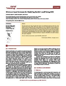
Daily streamflow observations for the period 2006-2008 were used to calibrate the REW model. For calibration, the Trial and Error procedure was applied where model parameters are manually changed and optimized with the objective to best simulate the streamflow observation time series. Optimization was done through changing one parameter at a time for each model run to control the effect on model behavior and performance. For calibration only model sensitive parameters are selected as shown in Reggiani and Rientjes (2005). Simple sensitivity was performed for these parameters prior to the actual calibration run. To warm the model for calibration, the year 2005 was selected. The performance of the model for each model run was evaluated with objective functions of Nash-Sutcliffe-Efficiency, volumetric error and a function Y that combines RVE and NSE.

27

USING SATELLITE-BASED RAINFALL ESTIMATES FOR RUNOFF MODELLING WITH THE REW APPROACH: APPLICATION TO THE UPPER GILGEL ABAY CATCHMENT

The calibration was done in three steps: first model was run with default model parameters for one year (2005) with in-situ measurements of precipitation, evapotranspiration and other climatological parameters for understanding the behavior of the model. The warming up helps to better simulate initial conditions and the simulation was started in the period of low flow which is the month of January. The second, the model was calibrated for the period 2006-2008 also using rainfall data from the rain gauges. The model parameter values are selected based on literature reviews and changed during calibration with considering their physical meaning in reality. While calibrating getting better match of the base flow between observed and simulated hydrograph was given primary concern. The next emphasis was better simulating peak flows of the observed hydrograph. After getting the better performing model results the precipitation forcing replaced with CMORPH inputs. The focus here is not on improving model simulation result when using SRE but rather comparing of model performance and simulation results when gauge based rainfall is replaced by SREs. More specifically, how well SRE represented the temporal dynamics of streamflow hydrograph like high flows. Sensitivity analysis of parameters was done with changing highly sensitive parameters (porosity, conductivities) which were identified in many model runs. Thus, the effect of these sensitive parameters in the performance of the model was also assessed. One year (2009) was used for validation of the model with in situ forcing. 5.2.1.1.

Model calibration

With the use of the default model parameter sets at the first run, a NS value of 0.12, a RVE of 8.95% and a Y of 0.11 was obtained. The model overestimated discharge with default model run. The simulated base flow not well matched with observed and the Peak discharges are overestimated. The system quickly reacts to rainfall forcing and there is mismatch between simulated and observed discharges especially in wet season. After a number of model runs for calibration, changes in the shape of hydrograph and improvements in Objective functions are noticed while changing some of the parameters. With an increase of exponent of precipitation partitioning from 0.28 to 0.45 and decrease of depth of saturated subsurface flow layer from 0.25m to 0.017 meter a major increase achieved which is NS 0.33 and RVE elevated from 8.95% to -1.70%. These parameter changes dampened of the peak discharges. Further improvement of NS and RVE was achieved with an increase of soil porosity from 0.5 to 0.6 and slight increase of saturated hydraulic conductivity from 0.0005 m/s to 0.008 m/s. With these changes the base flow well matched and the time to peak of some portions of the hydrograph in the beginning of dry season better matched.

28

USING SATELLITE-BASED RAINFALL ESTIMATES FOR RUNOFF MODELLING WITH THE REW APPROACH: THE CASE OF UPPER GILGEL ABAY CATCHMENT

Figure 19: Hydrograph showing the calibration result for 2006-2008

Results of model calibration are shown in Figure 19. Objective function values for final calibration are 0.71 for NS, 4.07% for RVE and 0.68 for Y. Values as such indicate a satisfactory model performance. Characteristic to the hydrographs are the relatively high discharges after periods of high intensity rainfall. The total Mass Error reported in the model simulation turns in to 2.4 x 10-9 after three year model run and indicates that all mass tracked and traced during a simulation. As shown in figure 19, the model simulates the initial condition and base flow well. The rising limb and recession limb are reasonably similar to the observed discharge. Most of the peak discharges in the year 2007 and 2008 are also simulated well. The model simulates peak flows in months of May and November (see figure 19) which can be associated with high precipitation events indicated but not shown in observed hydrograph. In contrast, it simulates some peaks which are not shown in the observed hydrograph. These might be associated with missing the high flows within these days in measuring or model structure. Overall, it can be concluded as base flow is well simulated for entire hydrograph. The peak discharges are also simulated well except some mismatches observed. 5.2.1.2.

Sensitivity Analysis

For sensitivity analysis many model runs were conducted to identify the parameters which are highly sensitive together with the referring the results of earlier works (e.g. Reggiani & Rientjes, 2005 and Zhang, et al., 2006). Three year model run which is similar to calibration was used for the sensitivity analysis. Highly sensitive parameters were changed manually at a time keeping less sensitive parameters unchanged. Finally, six cases which are close to the calibrated parameter sets in the performance selected and shown in Table 5. The result revealed that the model is highly sensitive to saturated hydraulic conductivities and porosity (soil parameter). It is also sensitive to depth of saturated subsurface flow layer. It is found that keeping the soil porosity similar and slightly increasing Ksat (see Table 5: cases I, II and II), enhances the model performance which allows better reproducing the peak flows of the hydrograph. In cases III and VI, the soil porosity increased from 0.45 to 0.6(which creates more storage to the system) and by keeping Ksat unchanged, the NS improved from 0.69 to 0.71. The sensitivity analysis results revealed subsurface parameters such as porosity and hydraulic conductivities are sensitive in affecting how well the model can simulate the stream flow discharges in Upper Gilgel Abay catchment.

29

USING SATELLITE-BASED RAINFALL ESTIMATES FOR RUNOFF MODELLING WITH THE REW APPROACH: APPLICATION TO THE UPPER GILGEL ABAY CATCHMENT

Table 5: Sensitivity analysis (2006-2008)

Model consistency

Soil porosity(-)

Saturated hydraulic conductivity (Ks)(m/s)

NS (NashSutcliffeEfficiency)

RVE (Relative volumetric error) (%)

Y

Case I

0.45

0.004

0.67

-7.02

0.63

Case II

0.45

0.015

0.67

13.00

0.59

Case III

0.45

0.008

0.69

2.64

0.68

Case IV

0.6

0.001

0.59

-17.44

0.51

Case V

0.6

0.004

0.69

-5.52

0.65

Case VI

0.6

0.008

0.71

4.07

0.68

5.2.1.3.

Model Validation

Because of the inter-annual rainfall variation and missing values observed in the year 2010 and 2011 only one year (2009) was used for validation of the model with rainfall inputs from rain gauges. For validation, the optimized parameter set by the calibration is used. Validation results indicate satisfactory model performance with objective function values for NS 0.62 and for RVE 9.59%. The latter indicates a relative high, positive, volumetric error. For the combination function Y a value of 0.57 was obtained, may be considered satisfactory. As shown in figure 20, the simulation result, peak flows and low flows are not always accurately simulated. However, the simulated hydrograph follows the general shape of the observed hydrograph.

Figure 20: validation hydrograph for the year 2009

30

USING SATELLITE-BASED RAINFALL ESTIMATES FOR RUNOFF MODELLING WITH THE REW APPROACH: THE CASE OF UPPER GILGEL ABAY CATCHMENT

5.3.

Runoff simulation with sattelte rainfall estimates forcing

CMORPH rainfall estimates were used as input to the REW as forcing term to evaluate how well the observed hydrograph can be simulated. Similar to the use of rainfall time series from rain gauges for model calibration, for the same period bias corrected CMORPH estimates are used. Results of modelling were evaluated by means of NS, RVE and Y is shown in Table 6. Table 6: Performance of CMORPH on runoff simulation forcing

NS(Nash-SutcliffeEfficiency)

RVE (Relative volumetric error) (%)

Y

CMORPH(2006-2008)

0.57

0.80

0.56

CMORPH(2006-2010)

0.43

13.71

0.38

CMORPH 2008

0.52

-4.81

0.50

CMORPH 2010

0.36

15.30

0.31

Figure 21: Streamflow simulation with bias orrected CMORPH rainfall estimates (2006-2010)

Based on the simulation result found, the base flow and most of the peaks follow a pattern of the observed hydrograph. Peaks for the years 2007-2010 are relatively well simulated (see figure 21). For the year 2006, the simulated hydrograph does not match with the measured discharge in many aspects like peak flows, rising limb and recession limb. For years 2007, 2009 and 2010, model simulation results do not well match for the rising and recession limbs as shown in measured streamflow (see figure 21). Recession starts much quicker for measured data for 2007, 2009 and 2010 indicating that SRE rainfall extends for a longer period compared to gauged rainfall. These differences in the model performance annually can be associated with the inter-annual rainfall variations and the difference in the performance of the satellite in detecting rainfall. A better performing model in simulating runoff is shown when using shorter time series (3) years (see Table 6).

31

USING SATELLITE-BASED RAINFALL ESTIMATES FOR RUNOFF MODELLING WITH THE REW APPROACH: APPLICATION TO THE UPPER GILGEL ABAY CATCHMENT

To better evaluate inter-annual differences in SREs year 2008 (that seems visually better) and 2010 (that appears to be poorer), are plotted in figure 22, left and right respectively. The year 2008 shows better results of NS (0.52) and RVE (-4.81). In 2008 higher peaks are shown at the start of the wet season but with good recession part. In 2010 rising limbs are better represented and the highest peaks are shown with mismatches (See also to Fig 22 for these patterns). The overall shape of the hydrograph also preserved well for the year 2008, where NS (0.52) and RVE (-4.81%) was obtained. While evaluating the year 2010 only, NS (0.36) and RVE (15.3%) was found, which can be taken as poor performance when compared to 2008. Overall, the performance of SREs follows the shape of stream flow hydrograph measured but varies annually.

Figure 22: Stream flow simulation with bias corrected CMORPH rainfall estimate (left; for the year 2008; and right; 2010)

5.4.

Identification of major runoff source with in the catchment

Saturated excess overland flow is the contribution of runoff which is generated from the saturated component of the REW areas. Rainy months of June, July, August and September (end of wet season) was taken for identifying the daily saturated excess overland flow contribution to the streamflow. The in-situ based streamflow simulation result was selected from SREs for analysis because of better model performance. Results of analysis of saturation excess overland flow are show in Figure 23 where for each REW (1-33) the overland flow depths is shown for the period 12 months (June, July, August and September 20062008). Average Depths result from accumulating the daily simulated overland flow depth was considered for analysis to indicate the REWs that mostly contribute to streamflow by saturation excess overland. The average depth ranges from 0-0.106 mm/day and REWs close to the river reaches are identified as high saturation excess generating areas (see figure 24). Areas in southern (REWs 19,20,21,22and 23) and south western(REWs 7,11,12 and 15) part of Upper Gilgel Abay catchment indicated an average saturated overland flow thickness of 0.018-0.051mm and in mountainous areas of REW 16,29 and 30 a value lower reported( 0-0.018 mm). Hence, spatial differences in signals of saturated excess overland flow identified with REW approach in Upper Gilgel Abay catchment.

32

USING SATELLITE-BASED RAINFALL ESTIMATES FOR RUNOFF MODELLING WITH THE REW APPROACH: THE CASE OF UPPER GILGEL ABAY CATCHMENT

Figure 23: Average Saturation excess thickness (mm) for REWs for wet season (months of June, July, August and September 2006-2008) per day

Figure 24: major runoff generation (saturation excess) source REWs

Three REWs (4, 13 and 25) selected for analysis, which generate high saturation excess overland flow compared to other REWs and displayed in Figure 24. REW 4 has area of 64.46 km2 which is 4.1 % of the total area of the catchment and is located in lowest elevation ranges 1918-2160m. REW 13 have area of 101.10 km2 which is larger area than the other two selected REWs (covers 7% area and found in elevation ranges of 1918-2214m). REW 25 also follows the other two. REW 25 has area of 75.21 km2 (covers 4.78 % and characterized as low elevation area (1896-2181m) compared to other REWs)). What makes all 3 REWs is the fact that these areas are very close to the outlet and river reach. For further analysis of where these REWs are located see Figure 24.

33

USING SATELLITE-BASED RAINFALL ESTIMATES FOR RUNOFF MODELLING WITH THE REW APPROACH: APPLICATION TO THE UPPER GILGEL ABAY CATCHMENT

Can locations of saturated excess overland flow areas be related to rainfall distribution? Average daily rainfall for the rainy months of June, July, August and September 2010 are plotted combined with average saturated excess overland flow from REWs 4, 13 and 25 that show highest saturation excess runoff (figure 25). A well-defined relation between rainfall and runoff is not shown although some days with high intensity rainfall also show high saturation excess runoff. However the result on the relation is somehow expected since the main driver for saturated excess overland flow is not rainfall rather it is associated with water table increase and when the water level reaches land surface and appears in the form of exfiltration. The correlation between average rainfall and saturated excess overland flow shows 0.0009, which indicates very little to no association (see figure 26).

Figure 25: Simulated saturated excess overland flow thickness for REW 4, REW 13, and REW 25

Figure 26: Correlation of REW average daily rainfall and Simulated saturated excess overland flow for REW 4, REW 13, and REW 25

34

USING SATELLITE-BASED RAINFALL ESTIMATES FOR RUNOFF MODELLING WITH THE REW APPROACH: THE CASE OF UPPER GILGEL ABAY CATCHMENT

5.5.

Comparision of high temporal resolution (hourly) and daily forcing on runoff simulation

800

0

700

5

Discharge(m3/s)

600 500 400

10

hourly rainfall

15

Simulated_hourly Simulated_daily

20

300

25

200

30

100 0 1-Jun-10

hourly rainfall(mm)

Temporal variability of rainfall with in Upper Gilgel Abay catchment reported in previous works as indicated in the background section. In this work CMORPH 8km × 8km and 1hr product was aggregated in to daily and used as forcing for stream flow simulation as discussed in section 5.2.3. However, hourly SRE was not tested as input for modelling stream flow in REW approach. The hourly simulation was done with keeping parameters and other climatological parameters similar to the respective daily time step. The analysis was done for three rainy months (June, July and August) of 2010, to better examine the difference in rainy season where differences in time step can be clearly observable on simulation. The resulting stream flow hydrograph for hourly time step is shown in figure 27. The result clearly shows the impact of time scale in the shape of stream flow hydrograph. The volumetric error found was -3.39%. This value can be taken as acceptable to make the comparison of the shape differences of the hydrograph. Average Lag time of 12.5 hours was found for 5 of the highest peaks observed in hourly simulation. The visual inspection of hourly simulation typically shows high flows which are not depicted in daily simulation and gauge measurements. These peaks are associated with high intensity rainfall event which last for short period and generate peak flows which might be missed during measurement. Aggregation of rainfall hourly SREs also totalizes these events as simple summation was used for daily time step. Overall, the shape of hourly simulation follows daily simulation as depicted in figure 27.

35 13-Jun-10

26-Jun-10

8-Jul-10 21-Jul-10 Time(date)

2-Aug-10

15-Aug-10

27-Aug-10

Figure 27: Comparison of hourly and the daily forcing on runoff simulation (June, July and August 2010) To better investigate the differences between hourly and daily SREs based simulations exceedance probability graphs was plotted and shown in figure 28. Exceedance probability defines the percentage of time that a given discharge can be equaled or exceeded. All simulated values were plotted in figure 28 to better capture the differences. The exceedance plots show clear differences in hourly and daily based simulations in peak flows and low flows (see figure 28). The differences in distribution of simulated values are evident for exceedance probabilities of