Modelling Annual Rainfall Using a Hidden-State Markov Model R Srikanthanab, M A Thyerc, G Kuczerad and T A McMahonbe a
d
Bureau of Meteorology, Melbourne , Australia 3000 (
[email protected])
b
Cooperative Research Centre for Catchment Hydrology, Monash University, Australia3800
c
Department of Forest Resources Management, University of British Columbia, BC, Canada
Department of Civil, Surveying and Environmental Engineering, University of Newcastle, Australia 2308 e
Department of Civil and Environmental Engineering, University Melbourne, Australia 3010
Abstract: In the past, stochastic modelling approaches generally assumed no variation in the parameters between years. There is a growing awareness of long term persistence in climatic data in the form of wetter and drier years. To take this information into account, model parameters should be varied in some way. The hidden-state Markov (HSM) model assumes that the climate is composed of two states, either a dry state (low rainfall year) or a wet state (high rainfall year). This approach provides an explicit mechanism for the HSM model to simulate the influence of quasi-periodic phenomenon such as ENSO. Separate distributions are used to model the rainfall in the two states. The states are not known a priori and are estimated along with the model parameters. For model calibration, a Bayesian framework is used to infer the distribution of the model parameters. A Markov Chain Monte Carlo method known as Gibbs sampler is used to estimate the parameters and their uncertainties. The HSM model was applied to 44 rainfall stations located in various parts of Australia and the results indicated that 32 stations are either highly likely to or could possibly have two states. One thousand replicates each of length equal to the historical data were generated and several model evaluation statistics computed. The HSM model satisfactorily preserved all the model evaluation statistics. Keywords: Annual rainfall; Hidden-state Markov model; Parameter uncertainty; Bayesian; 1.
dry spells observed in the data. Thyer and Kuczera [1999, 2000] developed a hidden-state Markov (HSM) model which explicitly assumes that the climate has two states. The HSM model was applied to annual rainfall data from 5 capital cities in Australia and it was found that only two cities, namely, Brisbane and Sydney exhibited two-state persistence.
INTRODUCTION
The modelling of annual rainfall data serves two purposes. Firstly, it enables the understanding of the stochastic nature of the annual rainfall data and its implications for long periods of low and high rainfall. This understanding is necessary to manage water supply systems during low rainfall periods. Secondly, any stochastic model should be able to maintain its statistical characteristics at different time scales and a good annual rainfall model allows one to disaggregate the generated annual rainfall data into monthly data. In this case, the annual data becomes the input to various disaggregation schemes.
The objective of the present study is to apply the HSM model to a large set of rainfall data from different climatic conditions and determine the extent to which two-state persistence exists in Australian annual rainfall data. Based on the analysis of both the Sydney rainfall data and stochastically generated data, Thyer and Kuczera [2000] observed that long-term records of data with length in excess of 120 years are required to detect two-state persistence. Notwithstanding this observation, it was decided to utilize 44 sites
The lag one Markov or the first order autoregressive model has been widely used to generate annual rainfall data [Srikanthan and McMahon, 1985, 2000]. The main drawback with this model is that it cannot model the long wet and
360
(Table 1) with long records (but shorter than that recommended by Thyer and Kuczera). The
selected sites adequately represent the different climatic conditions in Australia.
Table 1. Details of the rainfall stations used in the study. Number
Name
Latitude
Length Mean (years) (mm) 1005 Wyndham Port -15.46 128.10 79 695 2016 Lissadell -16.67 128.57 105 616 5008 Mardie -21.19 115.98 108 276 6036 Meedo -25.66 114.62 94 216 9034 Perth -34.93 138.58 115 868 10037 Cuttening -31.73 117.76 96 312 12065 Norseman Post Office -32.20 121.78 102 287 14902 Katherine Council -14.46 132.26 111 974 15540 Alice Springs Post Office -23.71 133.87 112 280 17031 Marree -29.65 138.06 113 164 19032 Orroroo -32.74 138.61 118 341 22020 Wallaroo -33.93 137.63 135 360 23000 Adelaide -31.95 115.84 139 530 24511 Eudunda -34.18 139.09 118 446 28004 Palmerville -16.00 144.08 109 1034 33035 Kalamia Estate -19.54 147.41 112 1085 35027 Emerald Post Office -23.53 148.16 108 642 36007 Barcaldine Post Office -23.55 145.29 112 496 39023 Cape Capricorn Lighthouse -23.48 151.23 87 801 39082 Rockhampton Post Office -23.40 150.50 96 946 40043 Cape Moreton Lighthouse -27.03 153.47 129 1550 40214 Brisbane -27.48 153.03 133 1154 41082 Pittsworth Post Office -27.71 151.63 112 703 42023 Miles Post Office -26.66 150.18 114 661 44026 Cunnamulla Post Office -28.07 145.68 120 374 47053 Wentworth Post Office -34.11 141.91 132 288 49002 Balranald RSL -34.64 143.56 121 322 54004 Bingara Post Office -29.87 150.57 113 745 62021 Mudgee (George Street) -32.59 149.58 122 670 66062 Sydney -33.86 151.20 140 1226 69018 Moruya Heads Pilot Station -35.91 150.15 123 972 72000 Adelong -35.31 148.06 115 795 72044 Tumut -35.30 148.22 113 822 75031 Hay Miller Street -34.52 144.85 119 369 77030 Narraport -36.01 143.03 112 354 80056 Tongala -36.25 144.95 69 443 81007 Caniambo -36.46 145.66 95 524 84030 Orbost -37.63 148.46 115 855 86071 Melbourne -37.81 144.97 143 657 86117 Toorourrong Reservoir -37.48 145.15 106 804 87043 Meredith (Darra) -37.82 144.15 124 685 91033 Frankford (Rossville) -41.32 146.73 106 1069 92012 Fingal -41.64 147.97 110 611 94061 Sandford (Maydena) -42.93 147.52 111 578 † Persistence structure: a – highly unlikely to have two-state persistence b – highly likely to have two-state persistence c – possibly to have two-state persistence
361
Longitude
Category† b a c b a a c a b c c c a c c b b b c b c c a c b b c c c b b a a b a c c c a a a b b b
2.
θ′ = ( µ W , σ W , µ D , σ D , P, S N
HIDDEN-STATE MARKOV MODEL
The HSM model (Figure 1) assumes the climate is in one of two states: wet (W) or dry (D). Each state has an independent rainfall distribution, assumed to be Gaussian. The time spent in each state is governed by the state transition probabilities. This provides an explicit mechanism to replicate variable lengths of wet and dry cycles.
)
(4)
Prior to model calibration the hidden-state time series is unknown. Thus it is included as a model parameter to be estimated during the calibration process. 3.
CALIBRATION OF HSM MODEL
For model calibration a Bayesian framework is used to infer the distribution of the model parameters, θ , for the given time series data, Y N . This distribution is referred to as the
P(W→D)
posterior distribution of the model parameters,
W
p ( θ Y N ) . Since the states are not known a
D
priori, it is not possible to derive an analytical expression for the posterior distribution. Thus Markov Chain Monte Carlo (MCMC) simulation methods are employed to draw samples from the posterior distribution. The basic idea of MCMC methods is to simulate a Markov chain iterative sequence, where at each iteration a sample of the model parameters, θ , is generated. Given certain conditions the distribution of these samples converges to a stationary distribution which is the
P(D→D)
P(W→W) P(D→W)
(
Figure 1. Schematic representation of the HSM model The simulation of annual rainfall time series is a two-step process. In the first step the climate state at year t, st, is simulated by a Markovian process: s t st -1 ~ Markov(P )
(1)
Several indices [Thyer, 2001] are used to interpret the results and these are briefly defined below. The wet and dry separation index (WADSI) is defined as
where P is a (2x2) state transition probability matrix whose elements are: pij = Pr (s t = j s t −1 = i )
i, j = W , D
(2) WADSI =
Once the state for year t is known, the rainfall is simulated using:
µW − µ D
(σ
2 W
+ σ D2 )
(5)
This index is a convenient measure of the separation between the wet and dry states. If the difference between the wet and dry means is large then the value of WADSI will be relatively high.
N( µ W , σ W2 ) if s t = W yt ~ 2 N( µ D , σ D ) if s t = D (3)
where N
)
posterior distribution, p θ Y N . To calibrate the HSM model, the MCMC method known as the Gibbs sampler is applied. The details of the calibration process are given in Thyer and Kuczera (2000) and it results in the expected values of the parameters with associated uncertainties.
(µ ,σ ) denotes a Gaussian distribution
The state signal index (SSI) is defined as follows:
2
with mean µ and variance σ . Therefore the vector of unknown parameters for the HSM model, θ , is composed of the rainfall distribution parameters for each state, the transition probabilities, and the hidden-state time series, S N = {s1 , s 2 ,...s N }, where: 2
SSI =
∑ P(W ) − 0.5 N
(6)
Values of SSI close to zero indicate no persistence in the rainfall to stay in either wet or dry state. Values of SSI around 0.3 generally indicates
362
persistence, but this needs to be confirmed with a visual inspection of a time series plot of the posterior probability of a year being classified as wet {P(st = W|YN).
posterior probability densities of WADSI and transition probabilities for one station from each of the three categories are shown in Figure 2. For Perth (Figure 2a), the two states are not identifiable as the posterior probability density function has its mode at zero. In addition, the two transition probabilities are not well defined and hence it is highly unlikely to have two-state persistence structure. For Meedo and Mardie, the two states are clearly identifiable as the probability of obtaining a value of zero or less for WADSI is zero or very small (Figures 2b and 2c). However, the two transition probabilities are well defined for Meedo (Figure 2b) only and it is highly likely to have two-state persistence structure. On the other hand, the two transition probabilities are not very well defined for Mardie (Figure 2c) and as a result it may not have two-state persistence structure.For a full set of results, the reader is referred to Srikanthan et al. [2002a]. By examining the expected residence times, SSI values and the posterior probability densities of WADSI and transition probabilities, 12 stations were categorised as highly unlikely to have two-state persistence structure. Of the remaining 32 stations, 15 stations indicated that it is highly likely to have two-state persistence and 17 stations could possibly have two-state persistence structure (Table 1). The locations of the three categories of stations are shown in Figure 3. The sites showing the existence of two-state persistence approximately correspond to the areas influenced by the ENSO, however we need to analyse more sites to clearly separate areas of two-state persistence from the rest.
The strength of the two-state persistence is assessed using the expected state resident times (SRT) and is obtained as the reciprocal of the transition probabilities.
E ( SRTD ) =
1 p DW
; E ( SRTW ) =
1 pWD
(7)
The posterior probability distributions of the transition probabilities are examined to see whether the transition probabilities are well defined. 4.
DISCUSSION OF RESULTS
The HSM model was calibrated to the 44 Australian rainfall stations (Table 1) and the indices described above were derived to interpret the results. As long records are needed to definitely detect the existence of two-state persistence structure, the rainfall stations were classified into the following three categories: (a)
Highly unlikely to have two-state persistence
The posterior probability density function of WADI has a mode less than or equal to zero. There is significant posterior probability mass for both pDW and pWD at = 0 and 1 so that the transition probabilities are not identifiable or posterior probability is fairly uniform over wide range of transition probabilities resulting in poorly identified transition probabilities.
Assuming the fitted model is correct, one thousand replicates each of length equal to the historic record were generated with parameter uncertainty for the 32 stations which exhibited two-state persistence structure. The mean, standard deviation, coefficient of skewness, lag one autocorrelation coefficient, extreme rainfalls and 2, 3, 5, 7 and 10-year low rainfall totals were calculated from each of the 1000 replicates. A full set of results is presented in Srikanthan et al [2002b]. The significance of the departures of the generated values from the corresponding historical values can be objectively assessed using the ratio (Hist – E[Gen])/sd(Gen) where Hist is the observed statistic, Gen is generated statistic, E[Gen] is the mean of the generated statistic and sd(Gen) is the standard deviation of the generated statistic. If the ratio is less than –2 or greater than 2, then the observed statistic is not consistent with the model. It can be seen from Table 2 that none of the ratio is outside the range (–2, 2). This shows that the model is consistent with the data.
(b) Highly likely to have two-state persistence To have two-state persistence, wet and dry distributions must be separate (high WADSI). There is zero or very small posterior mass for WADSI less than or equal to zero. Zero posterior probability mass for both pDW and pWD at = 0 and 1 and well defined transition probabilities so that the annual climate can move between states. (c)
Possibly have two-state persistence
All the remaining sites fall into this category meaning that the likelihood of two-state persistence is not clear; but possible. To determine the existence of two states, the empirical distributions of the difference in the means and the WADSI for the starting months having the largest WADSI were examined. The
363
0.06
0.025
0.05
Posterior density
Posterior density
0.030
0.020 0.015 0.010 0.005
P(W -> D)
P(D -> W)
0.04 0.03 0.02 0.01 0
0.000 0
0.5
1
1.5
0
2
0.2
0.4
0.6
0.8
1
Transition probability
WADSI
(a) Highly unlikely to have two-state persistence - Perth 0.09 0.08 0.07 0.06 0.05 0.04 0.03 0.02 0.01 0
Posterior density
Posterior density
0.025 0.020 0.015 0.010 0.005 0.000 0
0.5
1
1.5
P(W -> D)
0
2
0.2
0.4
0.6
P(D -> W)
0.8
1
Transition probability
WADSI
0.030
0.07
0.025
0.06
Posterior density
Posterior density
(b) Highly likely to have two-state persistence - Meedo
0.020 0.015 0.010 0.005
P(W -> D)
P(D -> W)
0.05 0.04 0.03 0.02 0.01 0
0.000 0
0.5
1
1.5
0
2
0.2
0.4
0.6
0.8
1
Transition probability
WADSI
(c) Possibly have two-state persistence - Mardie
Figure 2. The posterior probability densities of WADSI and transition probabilities.
5.
CONCLUSIONS
The hidden-state Markov model (HSM) which explicitly models the wet and dry states was applied to annual data from 44 rainfall stations located in various parts of Australia. Thirty-two stations exhibited two-state persistence structure. One thousand replicates were generated and several model comparison statistics were calculated. Comparison with the historical parameters shows that the HSM model preserves these statistics. It can be concluded that the HSM model is an improved model to generate annual rainfall data.
Figure 3. The locations of the stations those are highly unlikely to have two-state persistence (circles), highly likely to have two-state persistence (triangles) and possibly have two-state persistence (stars).
364
Table 2.
6.
The ratio of the model evaluation statistics.
Station
Mean
Std
Skew
Corre l
Wyndham Mardie Meedo Norseman Alice Springs Marree Orroroo Wallaroo Eudunda Palmerville Kalamia Emerald Barcaldine Cape Capricorn Rockhampton Cape Moreton Brisbane Miles Cunnamulla Wentworth Balranald Bingara Mudgee Sydney Moruya Hay Tongala Caniambo Orbost Frankford Fingal Sandford
-0.20 0.22 -0.09 -0.16 -0.12 -0.11 -0.25 -0.20 -0.21 -0.19 -0.10 -0.20 -0.17 -0.18 -0.12 -0.22 -0.15 -0.15 -0.09 -0.17 -0.21 0.35 -0.17 -0.12 -0.13 -0.22 -0.16 -0.16 -0.18 -0.20 -0.13 -0.16
dev -0.20 0.22 -0.09 -0.16 -0.12 -0.11 -0.25 -0.20 -0.21 -0.19 -0.10 -0.20 -0.17 -0.18 -0.12 -0.22 -0.15 -0.15 -0.09 -0.17 -0.21 0.35 -0.17 -0.12 -0.13 -0.22 -0.16 -0.16 -0.18 -0.20 -0.13 -0.16
0.35 -0.31 0.43 0.54 0.35 0.35 0.69 0.14 0.57 0.33 0.19 0.14 0.11 0.37 0.45 0.62 0.45 0.19 0.21 0.25 0.24 0.20 0.60 0.25 0.30 0.40 0.53 0.46 0.61 0.31 0.85 0.02
0.10 0.09 1.04 -0.34 1.24 0.20 0.23 -0.26 0.49 -0.03 -0.12 1.00 0.91 0.12 0.07 0.06 0.10 -0.62 0.23 0.52 0.73 0.10 0.30 0.41 0.31 0.93 1.05 0.15 -0.96 -0.07 0.41 -0.11
Extremes Max 0.41 -0.36 0.90 0.33 -0.12 0.18 0.86 -0.23 0.45 -0.10 -0.64 0.00 -0.60 -0.15 0.29 0.51 0.28 -0.12 0.15 0.21 0.34 0.03 0.54 -0.07 -0.12 0.32 0.36 0.33 0.19 -0.60 0.97 0.25
Min 0.47 0.82 1.35 0.98 0.86 1.24 1.02 0.85 1.02 1.05 1.74 0.28 -0.02 0.64 1.71 0.55 0.74 0.98 1.26 0.85 0.51 1.18 1.26 1.35 0.68 0.83 0.25 0.70 0.91 0.84 1.22 -0.53
Low rainfall sums 2 -0.23 -1.47 -0.03 0.19 0.51 -0.03 0.27 1.20 0.38 0.72 0.87 -0.78 -0.03 0.05 1.34 -0.72 0.49 -0.44 0.58 -0.60 -0.66 0.79 0.65 0.47 0.53 0.13 -0.98 0.12 0.61 0.97 0.31 -0.18
3 -0.35 -0.44 -0.06 0.69 0.98 0.44 0.13 1.03 0.01 0.16 -0.02 0.36 -0.03 -0.25 0.61 -0.63 0.96 0.04 -1.03 -0.97 -0.84 0.58 0.96 0.52 -0.13 -0.32 -1.50 -0.32 0.92 1.09 0.04 0.59
5 -0.47 -0.85 -1.31 0.24 -0.70 0.57 -1.18 -0.10 0.01 -0.14 -0.73 0.56 0.26 0.55 -0.10 0.56 0.70 -0.37 -1.43 -1.24 -0.28 -0.13 0.39 -0.51 -0.08 -0.35 -1.27 0.46 0.87 0.56 0.91 0.14
10 -0.68 -0.47 -0.08 0.74 -0.53 -0.80 -1.35 0.69 0.54 -0.54 0.14 0.46 0.30 -0.51 -0.53 0.09 -0.34 0.04 -0.24 -1.16 -0.45 -1.38 -0.72 0.08 -0.11 -0.79 -1.22 0.59 -0.02 0.71 -0.41 0.79
annual rainfall data, CRCCH Technical report (in press), 2002b. Thyer, M. A., Modelling long-term persistence in hydrological time series, Ph D Thesis, University of Newcastle, 2001. Thyer, M.A. and G. A., Kuczera, Modelling longterm persistence in rainfall time series: Sydney rainfall case study, Hydrology and Water Resources Symposium, Institution of Engineer, Australia: 550-555, 1999. Thyer, M. A. and G. A. Kuczera, Modelling longterm persistence in hydro-climatic time series using a hidden state Markov model, Water Resources Research, 36(11), 3301-3310, 2000.
REFERENCES
Srikanthan, R. and T. A. McMahon, Stochastic generation climate data: A review, CRCCH Report 00/16, Monash University, Clayton, 34pp, 2000. Srikanthan, R. and T.A McMahon, Stochastic generation of rainfall and evaporation data, AWRC Technical Paper No. 84, 301pp, 1985. Srikanthan, R., M.A. Thyer, G. A. Kuczera, and T. A. McMahon, Application of hidden state Markov model to Australian annual rainfall data, CRCCH Working Document (in press), 2002a. Srikanthan, R., G. A. Kuczera, M.A. Thyer, and T. A. McMahon, Stochastic generation of
365